Can a Universal Public Health Insurance Policy Dent Vulnerability to Poverty? Empirical Evidence from Rural India

Abstract

Idiosyncratic shocks, mainly health shocks, are common among rural households in developing countries, and as a result, many non-poor households fall into poverty and poor households remain poor. This study investigates the impact of a universal public health insurance policy, namely Rashtriya Swasthya Bima Yojana (RSBY), on household vulnerability to poverty (VtP) in rural India. Using 17,468 national-level household data, household VtP has been estimated using feasible generalised least squares (FGLS), and the impact of a health insurance policy on household VtP has been investigated using propensity score matching (PSM) and endogenous switching regression (ESR). FGLS estimates show that VtP is found to be 33 per cent compared to a currently classified poverty headcount rate of 27 per cent. PSM and ESR results indicate that access to RSBY significantly reduces household VtP, especially in less developed states.

JEL codes: I00, I13, I15, I18, I30, I32, I38, I39

Keywords

Rashtriya Swasthya Bima Yojana Vulnerability to poverty Health shocks Propensity-score matching Impact evaluation Health insurance India

1. Introduction

In developing countries, rural households are highly exposed to different types of shocks such as weather and demographic shocks (Dercon, 2005; Günther & Harttgen, 2009; Khosla & Jena, 2023). These shocks can cause households to remain in or fall into poverty due to their limited mitigating ability (Dercon, 2005; Günther & Harttgen, 2009; Khosla, 2022; Vo & Van, 2019). The shocks include loss of assets, jobs, floods, droughts and incidents such as disease and death (Carter et al., 2008). Among these, illness has always been at the forefront of the shocks tormenting poor households (Atake, 2018; Khosla et al., 2023; Vo & Van, 2019), and these households remain poor for an extended period due to a lack of access to health services and financial inability to seek hospitalisation and buy health insurance (DeLoach & Smith-Lin, 2018; Vo & Van, 2019). In India, public health insurance programmes have been introduced to help the poor access good-quality health services. However, there is little evidence on whether such health insurance policies—as a capacity enhancement tool—are able to reduce vulnerability to poverty (VtP) (DeLoach & Smith-Lin, 2018; Vo & Van, 2019).

Despite massive investment by the Indian government to provide health care services to its citizens, millions of people still fall into poverty every year due to poor health (Berman et al., 2010; Garg & Karan, 2009; Goyanka et al., 2019; Shahrawat & Rao, 2012). The situation is exacerbated by the fact that only 14 per cent of rural households are covered by any health insurance (Planning Commission, GoI, 2019). This figure of low insurance coverage underscores the critical role public health insurance policy could play in reducing poverty and VtP in India. Expanding the reach and effectiveness of these policies could not only mitigate health-related financial shocks but also improve overall economic resilience in rural areas.

Studies in India have mainly examined the impact of health policy on reducing out-of-pocket expenditure (OOPE), related to the implementation of the schemes and utilisation, and are mainly related to ex-post poverty reduction (e.g., Azam, 2018; Boyanagari & Boyanagari, 2019; Shahrawat & Rao, 2012; Singh & Kumar, 2017; Taneja & Taneja, 2016). Studies from other countries show a similar focus. In China, Lei and Lin (2009) found no reduction in OOPE or increase in healthcare utilisation, while Wagstaff et al. (2007) reported no impact on OOPE in Vietnam, and Ataguba and Goudge (2012) found no reduction in South Africa. However, other studies show positive effects. In China, Wagstaff (2010) and Axelson et al. (2009) reported reduced OOPE, with Wagstaff and Yu (2007) noting lower ex-post poverty. Galárraga et al. (2010) found healthcare insurance reduced OOPE for Mexico’s poor. In Ghana, Aryeetey et al. (2016) observed reduced OOPE, catastrophic expenditure and poverty. Liu and Zhao (2014) and Peng and Conley (2016) found health insurance lowered OOPE and increased utilisation in China, while Atake (2018) reported reduced VtP in South Africa. Similarly, Habib et al. (2016) highlighted reduced OOPE, borrowing and poverty across various contexts. However, there is relatively scant evidence of the economic impact of health insurance policy, especially on reducing VtP in developing countries in general and India in particular. One exception is Vo and Van (2019), who assessed VtP and found that health insurance reduces VtP in Vietnam.

This study investigates whether access to public health insurance policies reduces the likelihood of households falling into poverty in India. It contributes to the literature on estimating VtP and the role of social protection in reducing it in the following ways. First, unlike previous studies that provide an ex-post poverty impact of the health insurance programme, this study investigates the potential impact on ex-ante households VtP. Second, given the scant evidence of the impact of health insurance policy on ex-ante VtP, to the best of our knowledge, this study is the first to assess the impact of public health insurance policy on the reduction of VtP in India. The findings of the study provide causal impacts of Rashtriya Swasthya Bima Yojana and insights for possible revision of policies.

The remainder of the article is as follows: Section 2 explains the brief details of RSBY. Section 3 presents the material and methods used in the study. The interpretation of the findings is presented in Section 4. The concluding observations are presented in the final section.

2. Health Insurance Policies in India

The Indian government has implemented several health insurance policies since independence to help people who cannot afford private health insurance: for instance, the Employees’ State Insurance Scheme (ESIS) in 1948 and the Central Government Health Scheme (CGHS) in 1954. On 1 April 2008, the government launched a health insurance policy called Rashtriya Swasthya Bima Yojana (RSBY) intending to expand and help the poor and households working in unorganised sectors to access health facilities (Shahrawat & Rao, 2012). The goal of the scheme is two-fold: to provide financial protection against catastrophic health costs to the explicitly poor and workers belonging to unorganised sectors by reducing out-of-pocket hospitalisation expenses and to improve the access of poor households to quality health care.

Under the RSBY scheme, the government identifies households below the poverty line and those that belong to unorganised sectors are identified and issued a digital card to enrol them in the scheme. To identify beneficiaries, the government uses data from the National Sample Survey Organisation (NSSO) and household consumption/income. Further, employment-related household data collected by NSSO is used to identify households in unorganised sectors such as street vendors, beedi workers, Mahatma Gandhi National Rural Employment Guarantee Act (MNREGA) workers, sanitation workers, domestic workers, mineworkers and ragpickers.

Figure 1.

Conceptual Framework

Beneficiaries need to pay ₹30 per family as an annual registration fee at the time of enrolment. The scheme covers hospitalisation expenses up to ₹30,000 on a floater basis for a family of five. Transport charges of ₹100 per visit—up to a maximum of ₹1,000—are also provided (Shahrawat & Rao, 2012).

On 15 August 2018, the Indian government announced the Ayushman Bharat‑National Health Protection Mission (AB‑NHPM), which will incorporate the ongoing centrally sponsored RSBY scheme. However, nationwide household data is yet to come into public notice for analysis (Planning Commission, GoI., 2018b).

3. Material and Methods

3.1 Data Source

The data comes from the India Human Development Survey (IHDS) 2011–2012. The survey was carried out by the National Council of Applied Economic Research (NCAER), New Delhi, India, with technical support from Maryland University, USA. The IHDS data is nationally representative data that contains 42,362 household data across the country supplemented by individual data. In addition to detailed demographic information on household members, the survey includes data on assets, health issues, employment, migration and insurance policies (Desai et al., 2018).

We restrict our sample to rural household data because urban household data are not available for several states and union territories. Having cleaned the data by removing missing data and outliers, the final dataset for our study consists of 17,468 households.

Rural data is particularly relevant for our analysis because of the high incidence of poverty in these areas. Poverty is more pronounced in rural areas, where 25.70 per cent of the population is poor, compared to 13.70 per cent in urban areas. About 83.3 per cent of households still live in rural areas (Planning Commission, GoI, 2018a). Productivity and income in the agriculture sector are low compared to other sectors of the economy. Agricultural income contributes 18 per cent to the average annual gross income; however, more than 70 per cent of households in rural areas still depend on the agriculture sector for their livelihood (Planning Commission, GoI, 2011).

Since the poverty threshold level is necessary for the calculation of VtP, we have used a state-specific poverty line laid down by the Indian government. It comes from the state-specific poverty line for each state defined by the Suresh Tendulkar Committee for the year 2011–2012 (Planning Commission, GoI, 2014).

The poverty incidences are based on Foster et al. (1984). The equation is as follows:

P_{α} = \frac{1}{N} \sum_{i = 1}^{n} ({(\frac{z - y_{i}}{z})}^{α}) I (y_{i} < z)

(1)

where p_α is the Foster Greer and Thorbecke (FGT) index (0 > p_α < 1), N is the total number of sampled households considered for the study, z is the predetermined poverty line, y_i is the monthly per capita expenditure of the ith household, a is the FGT parameter that takes values of 0, 1 or 2, with different implications, and i is the individual household.

3.2 Analytical Framework and Econometric Specification

3.2.1 Conceptual Framework

Measuring vulnerability enables the identification of people who are not poor but may become poor, as well as those who will remain poor. Once identified, appropriate policies can be designed to prevent the former from falling into poverty and to help the latter to escape poverty. Clearly, measures that are focused on the current profile of poverty may be ineffective for those vulnerable individuals and households. By obtaining a vulnerability profile, both existing and future poverty can be targeted.

Economists define vulnerability as ‘exposure to negative shocks to welfare’ (Glewwe & Hall, 1998). One of the most popular approaches to measuring VtP is ‘vulnerability as expected poverty’ (VEP) developed by Chaudhuri et al. (2002), which uses cross-sectional data. The VEP model defines vulnerability ‘within the framework of poverty eradication, as the ex-ante risk that a household will, if currently non-poor, fall below the poverty line, or if currently poor, will remain in poverty’ (Chaudhuri et al., 2002).

Given the risks and shocks and lack of coping mechanisms, the government has undertaken several policy actions and interventions to either reduce or alleviate poverty through food security, employment, credit facilities and insurance for the poor and vulnerable (Azeem et al., 2019).

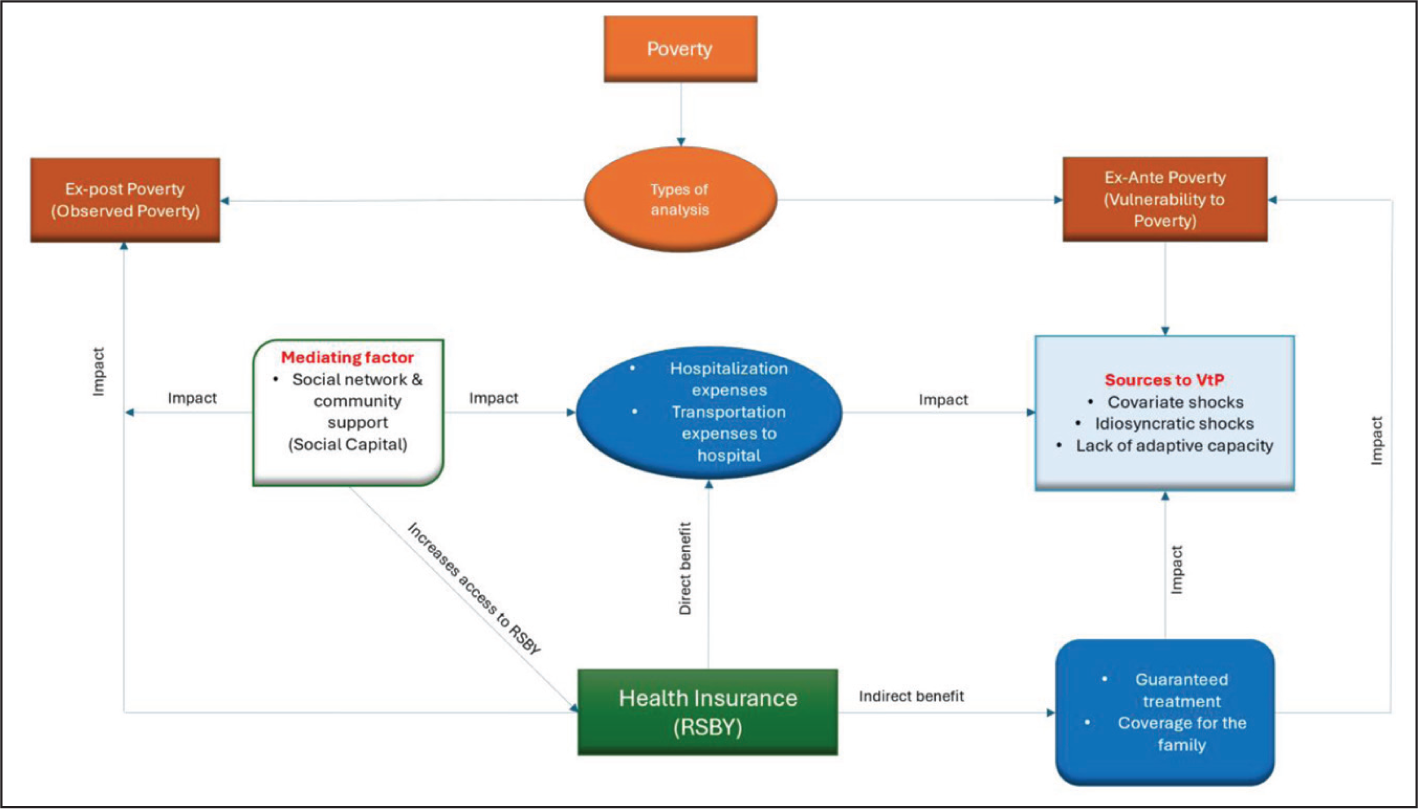
The conceptual framework of the study is presented in Figure 1. Poverty can be divided into two categories: ex-post poverty and ex-ante poverty. In the second part of the investigation, both ex-post and ex-ante vulnerabilities were estimated. Additionally, we utilised social capital as a mediating factor, which enhances access to RSBY by facilitating the dissemination of information and raising awareness about the social protection programme. This network-driven exchange of knowledge plays a crucial role in overcoming barriers to participation and improving the overall reach of the scheme. Finally, we investigated the effect of health insurance on the likelihood of being poor.

3.2.2 Vulnerability as Expected Poverty

The study estimated household vulnerability to expected poverty by employing the VEP approach devised by Chaudhuri et al. (2002). There is a growing body of evidence on estimating household VtP using this model (Chaudhuri et al., 2002; Günther & Harttgen, 2009; Jamal, 2009).

Given the absence of household panel data and detailed information on risks and shocks, the VEP approach has the advantage of estimating VtP by applying it to cross-sectional data. The following model has been adopted from the study by Chaudhuri et al. (2002).

The probability of household h being below the poverty line at time t + j. This can be expressed as

V_{h t} = P_{r} (\ln C_{h},_{t + j} < \ln z)

(2)

where V_ht denotes the vulnerability of a household at the present time t, P_r represents the probability of a household falling into poverty in a time of t + j, In C_h_, _{t + j} represents the future consumption level of household h at time t + j and z shows the pre-specified poverty line. To estimate VtP, a model must be defined (Haughton & Khandker, 2009). The model can be written as

\ln C_{h} = β_{0} + β_{1} X_{h} + e_{h}

(3)

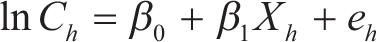
where C_h is the monthly consumption per capita of household h, β₀ is the intercept, β₁ is the slope coefficient, X_h is observable household characteristics (Table 1) and e_h is the zero-mean disturbance random error term that captures the variability of household consumption due to idiosyncratic factors. Chaudhuri et al. (2002) estimated VtP following the three-step feasible generalised least squares (FGLS) approach introduced by Amemiya (1977). We do not provide a detailed estimation of the VEP approach, as it is a standard approach to estimate VtP.

Table 1.

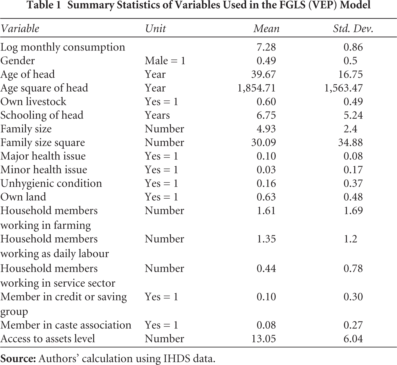
Summary Statistics of Variables Used in the FGLS (VEP) Model

Variable	Unit	Mean	Std. Dev.
Log monthly consumption		7.28	0.86
Gender	Male = 1	0.49	0.5
Age of head	Year	39.67	16.75
Age square of head	Year	1,854.71	1,563.47
Own livestock	Yes = 1	0.60	0.49
Schooling of head	Years	6.75	5.24
Family size	Number	4.93	2.4
Family size square	Number	30.09	34.88
Major health issue	Yes = 1	0.10	0.08
Minor health issue	Yes = 1	0.03	0.17
Unhygienic condition	Yes = 1	0.16	0.37
Own land	Yes = 1	0.63	0.48
Household members working in farming	Number	1.61	1.69
Household members working as daily labour	Number	1.35	1.2
Household members working in service sector	Number	0.44	0.78
Member in credit or saving group	Yes = 1	0.10	0.30
Member in caste association	Yes = 1	0.08	0.27
Access to assets level	Number	13.05	6.04

Source: Authors’ calculation using IHDS data.

After estimation of the expected mean and variance, VtP is estimated using the following equation:

{\overset{\land}{V}}_{h} = \overset{\land}{P_{r}} (\ln C_{h} < \ln z | X_{h} = Φ (\frac{\ln z - X_{h} \overset{\land}{β}}{\sqrt{X_{h} \overset{\land}{θ}}})

(4)

where is the estimated ex-ante vulnerability of household h, indicates the probability $\overset{\land}{V}$ that the household’s log consumption per capita (In C_h) will fall below the predetermined poverty line (In z). Φ represents the cumulative density function of the standard normal curve. $X_{h} \hat{β}$ and $\sqrt{X_{h} \overset{\land}{θ}}$ are the estimated mean and variance of household consumption, respectively.

Further, a vulnerable threshold must be defined to estimate vulnerable or non-vulnerable households, which is arbitrary and generally considered 0.5 (50 per cent probability) (Günther & Harttgen, 2009; Haughton & Khandker, 2009). The details on choosing VtP threshold are presented in Chaudhuri et al. (2002). This study used the vulnerability threshold of 0.5 to estimate vulnerable or non-vulnerable households.

3.2.3 Propensity Score Matching Approach

The propensity score matching (PSM) approach has been used in the present study to evaluate the impact of health insurance policy—RSBY—on household VtP. Cross-sectional data usually has non-experimental biases such as selection bias (Wooldridge, 2002). PSM corrects for selection bias by matching a sub-sample of access to RSBY and non-access to RSBY that have similar observable characteristics and by making comparisons in the region of common support (Becker & Ichino, 2002). The present study assessed the impact of RSBY on only VtP households (estimated using the FGLS approach), showing similar characteristics. The average treatment effect on the treated (ATT), which is the impact of RSBY on those VtP households that have access, has been estimated as follows:

A T T = E [Δ_{i} | T_{i} = 1] = E [Y_{1 i} | T_{i} = 1] - E [Y_{o i} | T_{i} = 1]

(5)

where T_i refers to treatment status of VtP household i and takes two values: t _i = 1 if a household has access to RSBY and t _i = 0 if a household does not have access to RSBY. Y ₁i = 1 is the VtP score if a household has access to RSBY, Y ₀i = 0 is the VtP score if a household does not have access to RSBY. E is the expectation operator and Δ_i is the treatment effect. ATT captures the change in the VtP score realised by households that have access to RSBY. The PSM approach used for the analysis has been detailed in other publications, such as Jena et al. (2017) and Jena and Grote (2017).

Matching requires building a new control group with similar characteristics so that for every treated observation (households with access to RSBY), there is an untreated one (households without access to RSBY). PSM constructs a probability that a household’s access to RSBY is conditional on its characteristics. This is done by running a logit model of ‘with access to RSBY’ and ‘without access to RSBY’ on the set of observable baseline characteristics. It can be written as

p (x) = p_{r} [T = 1 | X] = x_{i}, x_{2}, ...., x_{n}] = E (T | x)

(6)

where T = 1 for VtP households with access to RSBY and 0 for those without access to RSBY, and X is the vector of observable household characteristics, as presented in Table A2. Two assumptions have to be fulfilled to validate the matching: common support for the overlap and conditional independence. We have used three matching methods, namely the nearest neighbour, kernel and radius methods, where VtP households with access to RSBY have been matched with their neighbours based on the propensity score (PS).

3.2.4 Endogenous Switching Regression

We used endogenous switching regression (ESR) analysis to address hidden bias. ESR distinguishes two regimes: one for households that have accessed RSBY and the other for households that have not accessed RSBY. The ESR is estimated in two stages, and Equation (7) for the latent variable model is estimated as follows:

A_{i}^{*} = Z_{i} α + v_{i} w h e r e A_{t} = {_{0}^{1}_{o t h e r w i s e}^{i f Z_{i} α + v_{i} > 0}

(7)

When the expected gain of participation exceeds the value of non-participation, an i household participates in RSBY. Let A*_i be a latent variable that captures the benefit of participation by the ith household. Z_i is a vector of explanatory variables that describes how the regimes are selected. The parameter vector is α, and the error term is v_i. In the second step, the outcome equation is estimated. The first-stage selection equation’s observations are used to determine which of the two regimes to join. The outcome equations for the two regimes are as follows: accessed and non-accessed, corrected for endogenous selection:

Regime 1: Y_{1 i} = X_{1 i} β_{1} + σ_{1 u 1 i} {\overset{\land}{λ}}_{1 i} + u_{1 i} i f A_{i} = 1 (A c c e s s e d)

(7a)

Regime 2: Y_{2 i} = X_{2 i} β_{2} + σ_{2 u 2 i} {\overset{\land}{λ}}_{2 i} + u_{2 i} i f A_{i} = 0 (N o n ​ - ​ a c c e s s e d)

(7b)

In both regimes, where Y_1i and Y_2i, i = 1,….,N, represents the dependent variables. X_1i and X_2i are each regime’s explanatory variables, β₁ and β₂ are the parameters that need to be estimated, and the corresponding error terms are u_1i, u_2i. λ_1i and λ_2i are the inverse Mill’s ratios (IMR) estimated from the equation of first stage selection and used in the equations for correction of selection bias (7a) and (7b).

Four estimates are computed by the second-stage outcome regressions: (a) actual results from the accessed scenario, (b) real results of the non-assessed scenario, (c) counterfactual outcome scenario from accessed and (d) counterfactual outcome scenario for non-accessed. The ATT is computed as (a)–(c), and the average treatment effect on the untreated (ATU) is computed as (d)–(b).

4. Results and Discussion

4.1 Household Characteristics

Table 1 provides descriptive statistics on the variables used in the analysis. Results from demographic characteristics of respondents show that women household heads are in the majority (51 per cent), the mean age of household heads is about 40 years and their average years of schooling are about 7 years. Household members affected by a major health issue, such as a severe accident, as well as minor health issues, such as short sightedness, are also reported. At least 16 per cent of households live in a house that is considered unhygienic, 63 per cent have access to land and about 60 per cent own livestock. On average, 13 assets are held by the households.

More members work in farming, followed by those in the daily wage and service sectors. On social capital, 10 per cent and 7 per cent of households are part of savings and caste association groups, respectively.

4.2 Household Vulnerability to Poverty

4.2.1 Correlates of Vulnerability to Poverty

Table 2 presents the results for the estimates of ‘vulnerability as expected poverty’ using the FGLS approach. State dummies have been added to account for some of the unobserved factors arising from each state. Consistent with other studies, the coefficient for the years of schooling of the household head is positive and significant (Azeem et al., 2019; Günther & Harttgen, 2009; Jamal, 2009; Jena et al., 2024). Higher education of the household head plays a key factor in increasing consumption, reflecting that they have a higher per capita income.

Table 2.

Correlates of VtP

Variables	Log Monthly Consumption Coefficient	Std. Err.	Expected Consumption Coefficient	Std. Err.
Gender	–0.01	0.01	–0.10***	0.01
Age of head	0.00	0.00	0.08***	0.00
Age square	0.00	0.00	–0.00***	0.00
Own livestock	0.09***	0.01	0.22***	0.02
Schooling of head	0.00*	0.00	0.03***	0.00
Family size	–0.35***	0.00	–0.55***	0.01
Family size square	0.01***	0.00	0.03***	0.00
Major health issue	–0.03	0.05	–0.45***	0.07
Minor health issue	–0.02	0.02	–0.14***	0.04
Unhygienic condition	–0.01	0.01	–0.03	0.02
Own Land	0.07***	0.01	0.09***	0.01
Household members working in farming	0.05***	0.00	–0.01**	0.00
Household members working as daily labour	0.06***	0.00	–0.03***	0.01
Household members working in service sector	0.10***	0.00	–0.00	0.01
Member in credit or saving group	0.07***	0.01	0.08***	0.02
Member in caste association	0.07***	0.02	0.07***	0.02
Access to assets level	0.07***	0.00	0.08***	0.00
Himachal Pradesh	–0.81***	0.04	–0.72***	0.05
Punjab	–0.49***	0.04	–0.55***	0.05
Uttarakhand	–0.81***	0.05	–0.85***	0.07
Haryana	–0.46***	0.03	–0.41***	0.05
Rajasthan	–0.47***	0.03	–0.50***	0.05
Uttar Pradesh	–0.36***	0.03	–0.21***	0.05
Bihar	–0.35***	0.04	–0.29***	0.06
Assam	–0.47***	0.04	–0.261***	0.06
West Bengal	–0.70***	0.04	–0.54***	0.05
Jharkhand	–0.57***	0.04	–0.45***	0.06
Odisha	–0.79***	0.04	–0.67***	0.05
Chhattisgarh	–0.90***	0.04	–0.77***	0.06
Madhya Pradesh	–0.55***	0.03	–0.33***	0.05
Gujarat	–0.47***	0.04	–0.35***	0.06
Maharashtra	–0.65***	0.03	–0.64***	0.05
Andhra Pradesh	–0.48***	0.05	–0.47***	0.06
Karnataka	–0.50***	0.03	–0.39***	0.05
Kerala	–0.56***	0.04	–0.47***	0.06
Tamil Nadu	–0.82***	0.05	–0.66***	0.06
Constant	7.99***	0.04	6.54***	0.70
Adjusted R square	0.6489		0.5786
Observations	17468		17468

Source: Authors calculation using IHDS data.

Note: Asterisks denote the following: ***significant at 1% level.

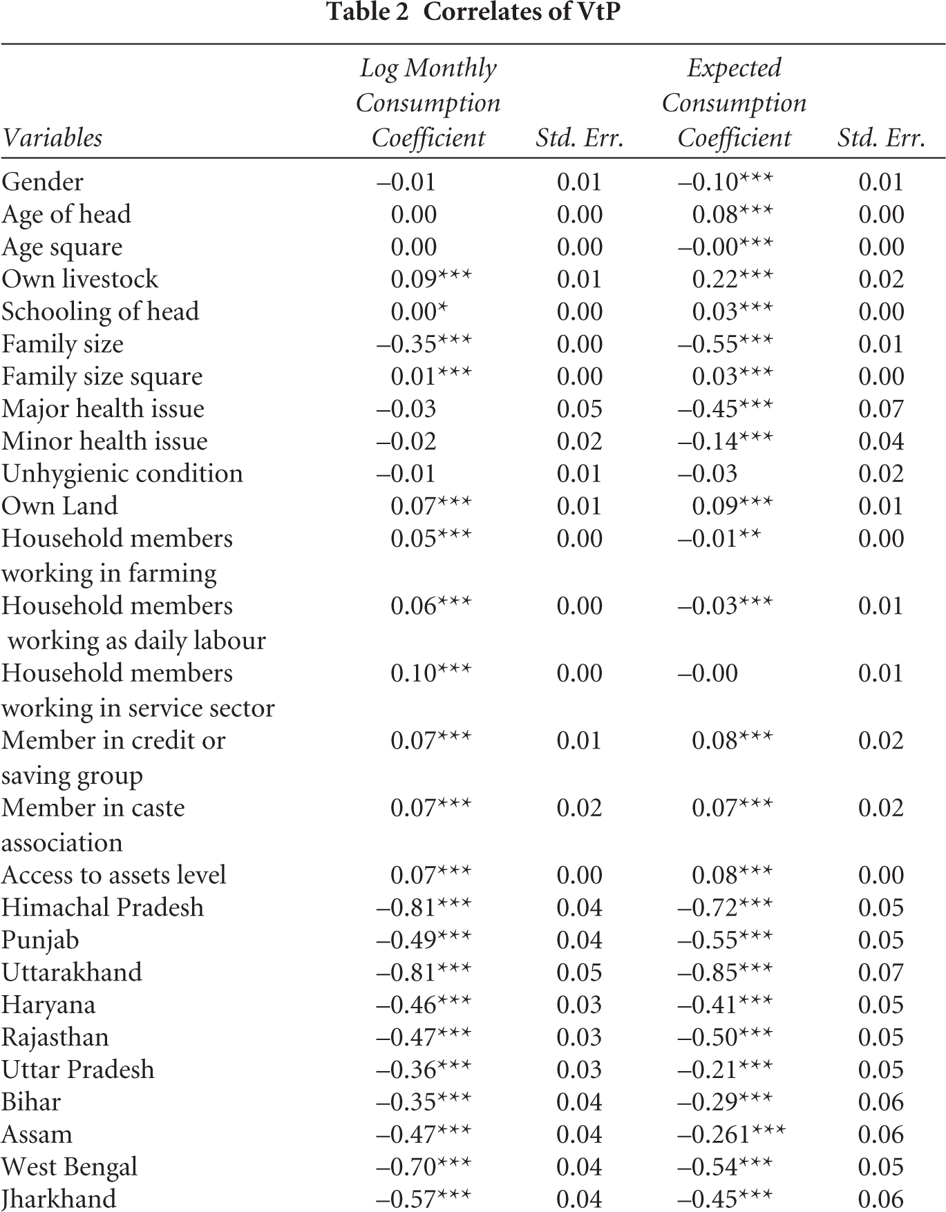
With respect to household size, the coefficient of household size is negative and significant, but its squared term (household size square) shows a positive association with household well-being, suggesting a non-linear association with consumption per capita. This finding is consistent with the past empirical VtP studies, which observed a negative association between household size and household consumption expenditure (Azeem et al., 2019; Jamal, 2009). The results also show that ownership of livestock increases consumption in the household by 9.3 per cent. Generally, livestock is considered to be a major livelihood asset in rural areas that works as a major coping strategy during adverse events.

On household occupation, households are generally categorised as the number of members working in farming, daily wage and service sectors. The findings show that the coefficients of household members working in all these sectors are positively significant, suggesting a positive association with consumption per capita. However, as observed from Table 2, household members in the service sector are more likely to increase consumption than with farming and daily wage earners. The regression results also indicate that the land ownership coefficient is positive and significant, which suggests that keeping other factors constant, ownership of land increases the household consumption level. This finding is consistent with previous studies that observed a positive association between land ownership and consumption per capita (Iqbal, 2013; Jha & Dang, 2009).

Social capital within the community is expected to play a key role in disseminating information. Social capital plays a significant role in escaping poverty and reducing VtP (Khosla & Jena, 2020, 2022). The findings show that households that are members of saving and caste association social groups are more likely to increase consumption by 6.7 per cent and 7 per cent, respectively. The regression results also indicate that households that possess more assets are more likely to increase their consumption level by 7 per cent. This finding is consistent with a study that observed lower vulnerability for households with higher assets (Jha & Dang, 2009). Recently, the estimation of poverty has been shifted to asset ownership, suggesting that households with better access to assets have more chances to escape poverty (Carter et al., 2008). Our findings bring further evidence of the criticality of maintaining a strong asset base to reduce poverty and vulnerability. In the case of the state dummy, states provide different levels of facilities to the population, with developed states providing better facilities to households.

4.2.2 Vulnerability Estimates

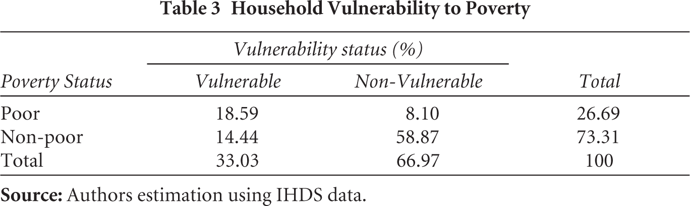
The estimates from the FGLS show that 33 per cent of the households have a greater than 50 per cent chance of falling into poverty (Table 3). The results show that the percentage of vulnerable households exceeds that of the currently classified poor by 27 per cent. This finding is consistent with previous VtP studies (Azeem et al., 2019; Chaudhuri et al., 2002; Vo & Van, 2019). Further, about 19 per cent of poor households are likely to fall into extreme poverty, and 14 per cent of non-poor households are likely to fall into poverty. Although the rate of households likely to remain poor is relatively high, the incidence of households at risk of falling into poverty underscores the importance of health shock in rural India. The findings suggest that policies that target only the poor should also consider VtP households to reduce the likelihood of falling into poverty.

Table 3.

Household Vulnerability to Poverty

Poverty Status	Vulnerability status (%)		Total
Poverty Status	Vulnerable	Non-Vulnerable	Total
Poor	18.59	8.10	26.69
Non-poor	14.44	58.87	73.31
Total	33.03	66.97	100

Source: Authors estimation using IHDS data.

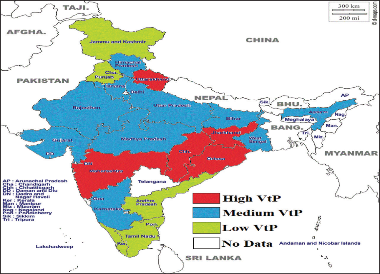
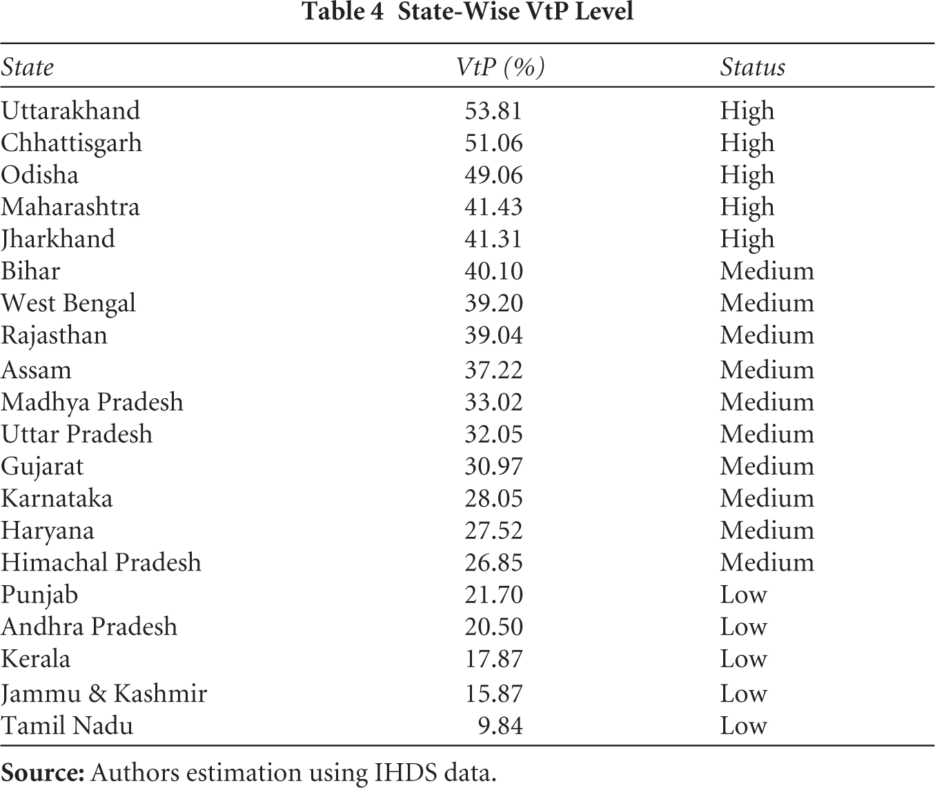
The VtP estimation shows that households in economically backward states are more vulnerable (Figure 2 and Table 4). Uttarakhand, Chhattisgarh, Odisha, Maharashtra and Jharkhand are extremely vulnerable states where between 40 per cent and 54 per cent of households have a chance of falling into poverty, whereas Tamil Nadu, Jammu & Kashmir, Kerala and Andhra Pradesh are less vulnerable states. This suggests that households in developed states are better at accessing public facilities for health and transportation, which are provided in a developed state and help reduce poverty (Charlery et al., 2016).

Figure 2.

Source: Authors’ design using IHDS data.

Table 4.

State-Wise VtP Level

State	VtP (%)	Status
Uttarakhand	53.81	High
Chhattisgarh	51.06	High
Odisha	49.06	High
Maharashtra	41.43	High
Jharkhand	41.31	High
Bihar	40.10	Medium
West Bengal	39.20	Medium
Rajasthan	39.04	Medium
Assam	37.22	Medium
Madhya Pradesh	33.02	Medium
Uttar Pradesh	32.05	Medium
Gujarat	30.97	Medium
Karnataka	28.05	Medium
Haryana	27.52	Medium
Himachal Pradesh	26.85	Medium
Punjab	21.70	Low
Andhra Pradesh	20.50	Low
Kerala	17.87	Low
Jammu & Kashmir	15.87	Low
Tamil Nadu	9.84	Low

Source: Authors estimation using IHDS data.

However, households in developed states can also fall into poverty. The heterogeneous impact of policies and other adverse events can pull many households into poverty. Maharashtra fell among the top VtP states. The possible reasons could be severe health issues in rural areas, followed by adverse events such as recurring drought. In this study, we consider only household consumption per capita as the well-being indicator, which may differ when we use HDI indicators (education, health and the standard of living) to estimate VtP.

Chhattisgarh, Odisha and Jharkhand are known for the high poverty rate. In these states, economic growth and development are quite retrograde. Households in these states are mostly dependent on the agriculture sector, literacy rates are low (Planning Commission, GoI, 2011) and infant mortality rate (IMR) is high (NIMS, ICMR, & UNICEF, 2012).

4.3 Impact of Health Insurance on VtP

This section explains the empirical results of PSM. The comparison among adopters and non-adopters of RSBY and the determinants of RSBY adoption are presented in Tables A1 and A2.

4.3.1 Uptake of RSBY Across States

Figure 3 represents the state-wise household access to RSBY. There is a significant difference in the distribution of RSBY cards among states: Andhra Pradesh (86.1 per cent) has the highest fraction of households with access to RSBY cards, while Tamil Nadu (1.43 per cent) has the lowest. The top five states in terms of percentage of access to RSBY cards are Kerala (42.61 per cent), Bihar (29.88 per cent), Chhattisgarh (27.77 per cent) and Uttarakhand (25 per cent), whereas Assam (2.75 per cent), Punjab (3.51 per cent), Jammu & Kashmir (4.46 per cent) and Maharashtra (5.62 per cent) sit at the bottom.

Figure 3.

Source: Authors’ calculation using IHDS data.

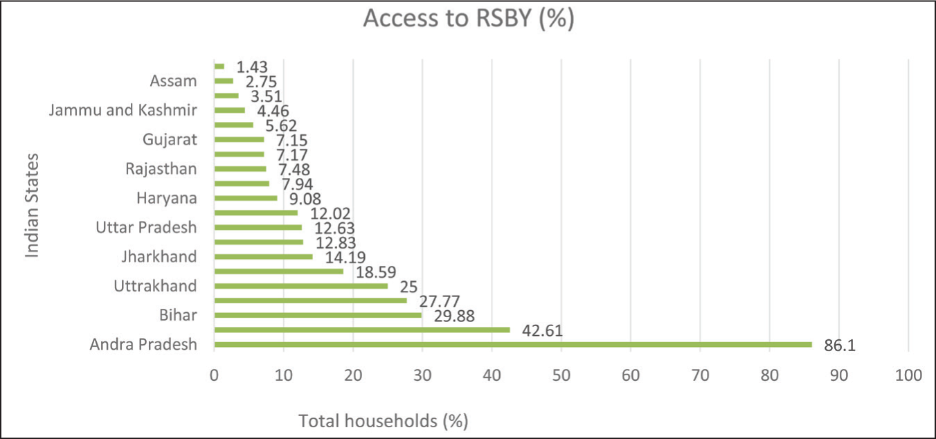
It is also observed that RSBY card distribution is lower for many less-developed states such as Assam, Odisha and Rajasthan. In contrast, households in developed states such as Kerala, Uttarakhand and West Bengal have higher access to RSBY cards. Chakrabarti and Shankar (2015) show that there is a heterogeneous distribution of RSBY cards within the country.

4.3.2 Impact of RSBY on Household VtP

To assess the impact of public health insurance policy on household VtP, we first analysed the entire VtP dataset. However, the results were not significant. We then divided the states into two categories of less developed and developed states using an HDI value of 0.5 as the cut-off (Planning Commission, GoI, 2011) and performed the estimation for both categories. The results are statistically significant only for less developed states.

Table 5 reports the average effects of accessing RSBY on household VtP, estimated using the PSM approach. All three estimators—nearest neighbours (5), kernel matching and radius matching—yield similar results. For all the first-stage logit model’s explanatory variables, the differences after matching are statistically insignificant, which is a desired property for a good matching algorithm, which shows that the results are reliable. For the three matching methods, the PS graphs are shown in Figure 4.

Table 5.

Impact of RSBY on Household VtP, PSM Results

Outcome Variable	Matching Estimator	Least-Developed States		Developed States		Total sample
Outcome Variable	Matching Estimator	ATT	t-Test	ATT	t-Test	ATT	t-Test
Vulnerability	Nearest neighbour	–0.017	2.54**	–0.006	–0.74	–0.002	–0.44
	Kernel matching	–0.014	2.34**	0.003	0.33	–0.003	–0.78
	Radius matching	–0.014	2.34**	0.002	0.28	–0.003	–0.76
	Observations	3,210		2,560		5,770

Source: Authors estimation using IHDS data.

Note: Asterisks denote the following: **significant at 5 per cent level.

Figure 4.

Source: Authors’ calculation using IHDS data.

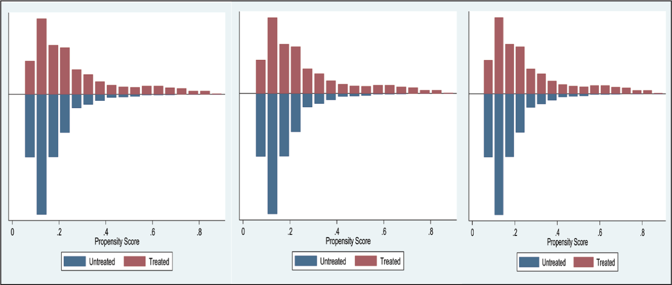
Table 5 also shows the ATT of accessing RSBY for VtP households in developed states, less developed states and the whole VtP sample. Accessing RSBY reduces VtP for all groups, but it is found to be statistically significant only for households in less developed states (states that have a lower HDI). The results indicate that households’ access to RSBY helps them cope with health shocks. Under all three algorithms, the decrease in VtP score ranges from 1.4 per cent to 1.7 per cent. These findings are consistent with previous studies on the impact of health insurance on VtP. Atake (2018) observed that access to health insurance reduces VtP in three African countries, namely Burkina Faso, Niger and Togo. Recently, Vo and Van (2019) have shown that health insurance reduces VtP in Vietnam with a 16 per cent reduction of VtP.

The findings in our study show that the public health insurance policy in India has a partial impact on VtP; that is, access to RSBY has resulted in a decline in VtP in less developed states (states with a lower HDI) compared to developed states. One possible reason for this finding could be the better infrastructure facilities available in developed states. Better facilities in terms of sanitation, roads and other facilities can result in higher income (Charlery et al., 2016). In developed states, rural households have access to free and better health care near their residents. The better-connected transportation facilities help them avail themselves of treatment at the early stage of health issues. However, given the poor living standards, it is quite difficult for poor households to spend on even a minor health issue. Further, considering the poor infrastructure facilities in rural areas, visiting a health centre may take an entire day to avail of the treatment. Since RSBY also provides transportation charges, it helps very poor households from less developed states. Another possible reason could be the poor standard of living of households in backward states. Poor people cannot afford to buy adequate amounts of nutritious food, preventive and curative health care, quality and affordable housing and education (Atake, 2018).

4.4 Results from the ESR Model

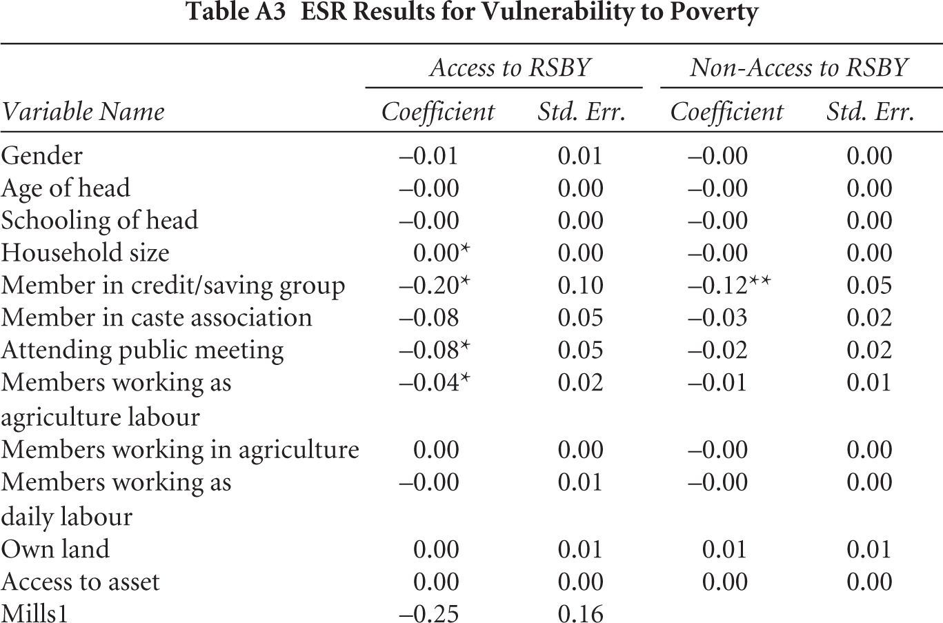
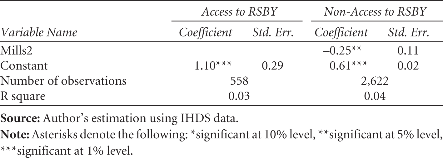
As the results of the PSM model may be biased due to unobserved factors, the ESR model was used to check the robustness of the estimated effects obtained from the PSM model. The advantage of the ESR model over the PSM model is that it can estimate the potential gain for the non-accessed had they accessed RSBY. The ATT and ATU of RSBY estimated from the ESR models are presented in Table 6, and the second stage ESR estimation results are presented in Table A3. These estimates corroborate the PSM model findings, showing that the ESR-based ATU is close to PSM-based estimates. There is a negative and statistically significant ATT of RSBY on household VtP, especially for the less developed and total VtP sample households. More specifically, the VtP effect for the RSBY access is –0.03 and –0.01, suggesting that RSBY reduces their probability of falling below the poverty line by 3 per cent and 1 per cent, respectively. Similarly, the ATU for the non-accessed is positive, indicating that if they had decided to access RSBY, their household VtP would have declined.

Table 6.

Impact of RSBY on Household VtP, ESR Results

Outcome Variable	Category	Rural India
		Impact of RSBY on VtP Households (Less Developed States)		Average Treatment Effect	Impact of RSBY on VtP Households (Developed States)		Average Treatment Effect	Impact of RSBY on VtP Households (Total VtP Sample)		Average Treatment Effect
		To Access	Not to Access	Average Treatment Effect	To Access	Not to Access	Average Treatment Effect	To Access	Not to Access	Average Treatment Effect
Vulnerability	ATT	(a) 0.66 (0.00)	(c) 0.69 (0.00)	–0.03*** (0.00)	(a) 0.65 (0.00)	(c) 0.65 (0.00)	0.00** (0.00)	(a) 0.65 (0.00)	(c) 0.66 (0.00)	–0.01*** (0.00)
	ATU	(d) 0.66 (0.00)	(b) 0.66 (0.00)	0.00 (0.00) ***	(d) 0.66 (0.00)	(b) 0.65 (0.00)	0.01 (0.00) ***	(d) 0.66 (0.00)	(b) 0.66 (0.00)	0.00 (0.00) ***

Source: Authors’ estimation using IHDS data.

Note: **significant at 5% level, ***significant at 1% level.

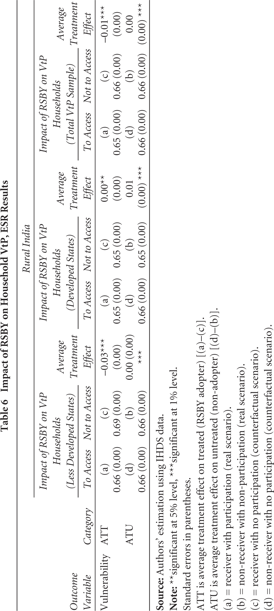
Standard errors in parentheses.

ATT is average treatment effect on treated (RSBY adopter) [(a)–(c)].

ATU is average treatment effect on untreated (non-adopter) [(d)–(b)].

(a) = receiver with participation (real scenario).

(b) = non-receiver with non-participation (real scenario).

(d) = non-receiver with no participation (counterfactual scenario).

In the case of developed states, the ATT is positive and significantly associated with VtP (ATT = 0.00), which implies that the participation of households in RSBY has not reduced their probability of falling below the poverty line. This result corroborates the PSM estimates, which suggest that access to RSBY has no significant impact in developed states.

4.5 Confounding Factors: The Role of Rapid Economic Growth and Key Economic Policies (2000–2010)

The results suggest that households with access to RSBY are less likely to fall into poverty. However, the implementation of RSBY in India from 2008 onwards coincided with a period of rapid economic growth and significant economic policy changes, introducing several confounding factors that may have influenced its outcomes. During the 2000–2010 decade, India experienced robust economic growth, averaging about 6–7 per cent annually (Ministry of Finance, GoI, 2024). This economic surge led to increased household incomes, improved living standards and greater access to services, which could have indirectly enhanced the effectiveness of RSBY. For instance, higher household incomes might have improved the ability of beneficiaries to utilise health services, while economic growth likely spurred investments in healthcare infrastructure, both from private and public sources. Such improvements would enhance the healthcare environment in which RSBY operated, making it difficult to attribute changes in health outcomes or poverty reduction solely to the insurance scheme.

Moreover, various economic policies implemented during this period, such as the National Rural Health Mission (NRHM), Mahatma Gandhi National Rural Employment Guarantee Act (MGNREGA) and Public Distribution System (PDS), also likely influenced RSBY’s impact. These policies aimed to improve healthcare delivery, increase employment, provide food security and reduce poverty, thereby providing complementary benefits to RSBY’s objectives. For example, NRHM aimed to strengthen rural healthcare infrastructure, potentially increasing the availability and quality of services for RSBY beneficiaries. Similarly, MGNREGA helped increase rural incomes, which could enable households to afford indirect healthcare costs not covered by RSBY. The PDS aimed to improve the quality of life in rural areas by providing affordable access to essential food grains, thereby reducing hunger and enhancing food security for low-income households. Therefore, the observed outcomes may be the result of a combination of RSBY and these broader policy interventions, complicating causal inference. Although we controlled for state-level heterogeneity using state dummies, fully isolating the effect of RSBY requires more rigorous methods. Future studies should consider employing advanced econometric techniques, such as difference-in-differences (DiD) or instrumental variable (IV) approaches, to better disentangle the effects of RSBY/public health insurance policy from the broader socio-economic changes and policy interventions.

4.6 Limitations of the Study

The econometric approaches employed in the study, such as PSM and ESR, offer notable advantages in estimating impact evaluation. While the model controls selection bias arising from both observed and unobserved factors to quantify the impact evaluation of RSBY when employing cross-sectional data, they still face potential challenges. The experimental approach is regarded as the gold standard; nonetheless, acquiring such data is infrequent. Hence, the integration of panel data and methodologies such as DiD augments the precision of estimated values and fortifies the credibility of the findings.

Another limitation arises from potential biases in data collection and reporting. Households benefiting from multiple programmes might over-report improvements, while those less impacted by economic growth or policy measures may under-report benefits. Though we used state dummies to control such unobserved factors, future research should use more robust methodologies, such as randomised controlled trials, DiD or IV regression econometric techniques to better isolate RSBY’s effects amid these confounding factors.

5. Summary and Conclusion

The available quantitative evidence of the impact of health policy on reducing the likelihood of falling into poverty is scant. Using the PSM and ESR econometric approaches, we contribute empirical evidence for the impact of a health policy —RSBY—on reducing VtP in rural India. The findings indicate that households that have access to RSBY are better able to cope with the situation than households without it.

The empirical part of this article follows two steps. In the first step, the FGLS econometric approach has been applied to estimate household VtP using nationally representative data from rural India. The FGLS analysis identifies key factors that reduce VtP, including education, livestock ownership, landholding, social capital and employment in the service sector. Among the states analysed, Uttarakhand, Chhattisgarh, Odisha, Jharkhand and Maharashtra stood at the top of the VtP states, linked to economic backwardness and low adoption of public health insurance (RSBY). The second step investigates the impact of RSBY on VtP using PSM and ESR methods. The results consistently show that RSBY significantly reduces VtP, particularly in less developed states. In contrast, RSBY appears to have no noticeable impact in developed states.

Our findings lead to policy implications for VtP reduction in rural India, given that the government is planning to promote public health insurance to protect the low-income group from health shocks. States like Assam, Odisha and Rajasthan have less uptake of RSBY, suggesting the need to upgrade the RSBY system by improving the coverage, enrolment practices, awareness and provision of better service in these states. Identifying the right beneficiaries is a significant challenge even now; a significant proportion of identified beneficiaries is excluded from the list in almost every state (Boyanagari & Boyanagari, 2019; Chakrabarti & Shankar, 2015; Taneja & Taneja, 2016). From the findings, we recommend a forward-looking approach (VtP approach) to identify beneficiaries, as it correctly estimates the different categories of VtP.

Such a forward-looking approach requires a data-driven approach in which precise data regarding livelihood choices, assets, income and consumption are collated to identify vulnerable households. Finally, considering the partial impact of RSBY and limited study on VtP reduction, further research is needed to understand the welfare effect of health insurance policy in India in VtP reduction. We, therefore, recommend further research on the impact of health policy on VtP in India using panel data.

Footnotes

Declaration of Conflicting Interests

The authors declared no potential conflicts of interest with respect to the research, authorship and/or publication of this article.

Funding

The authors received no financial support for the research, authorship and/or publication of this article.

Appendix

Table A3.

ESR Results for Vulnerability to Poverty

Variable Name	Access to RSBY		Non-Access to RSBY
Variable Name	Coefficient	Std. Err.	Coefficient	Std. Err.
Gender	–0.01	0.01	–0.00	0.00
Age of head	–0.00	0.00	–0.00	0.00
Schooling of head	–0.00	0.00	–0.00	0.00
Household size	0.00*	0.00	–0.00	0.00
Member in credit/saving group	–0.20*	0.10	–0.12**	0.05
Member in caste association	–0.08	0.05	–0.03	0.02
Attending public meeting	–0.08*	0.05	–0.02	0.02
Members working as agriculture labour	–0.04*	0.02	–0.01	0.01
Members working in agriculture	0.00	0.00	–0.00	0.00
Members working as daily labour	–0.00	0.01	–0.00	0.00
Own land	0.00	0.01	0.01	0.01
Access to asset	0.00	0.00	0.00	0.00
Mills1	–0.25	0.16
Mills2			–0.25**	0.11
Constant	1.10***	0.29	0.61***	0.02
Number of observations	558		2,622
R square	0.03		0.04

Source: Author’s estimation using IHDS data.

Note: Asterisks denote the following: *significant at 10% level, **significant at 5% level, ***significant at 1% level.

References

Amemiya

(1977). The maximum likelihood and the nonlinear three-stage least squares estimator in the general nonlinear simultaneous equation model. Econometrica: Journal of the Econometric Society, 45(4), 955–968. https://doi.org/10.2307/1912684

Aryeetey

G. C.

, Westeneng

, Spaan

, Jehu-Appiah

, Agyepong

I. A.

, & Baltussen

(2016). Can health insurance protect against out-of-pocket and catastrophic expenditures and also support poverty reduction? Evidence from Ghana’s National Health Insurance Scheme. International Journal for Equity in Health, 15(1), 116.

Ataguba

J. E. O.

, & Goudge

(2012). The impact of health insurance on healthcare utilisation and out-of-pocket payments in South Africa. The Geneva Papers on Risk and Insurance-Issues and Practice, 37(4), 633–654.

Atake

E. H.

(2018). Health shocks in Sub-Saharan Africa: Are the poor and uninsured households more vulnerable? Health Economics Review, 8(1), 26.

Axelson

, Bales

, Minh

P. D.

, Ekman

, & Gerdtham

U. G.

(2009). Health financing for the poor produces promising short-term effects on utilization and out-of-pocket expenditure: Evidence from Vietnam. International Journal for Equity in Health, 8(1), 20.

Azam

(2018). Does social health insurance reduce financial burden? Panel data evidence from India. World Development, 102, 1–17. https://doi.org/10.1016/j.worlddev.2017.09.007

Azeem

M. M.

, Mugera

A. W.

, & Schilizzi

(2019). Do social protection transfers reduce poverty and vulnerability to poverty in Pakistan? Household level evidence from Punjab. The Journal of Development Studies, 55(8), 1757–1783. https://doi.org/10.1080/00220388.2018.1448068

Becker

S. O.

, & Ichino

(2002). Estimation of average treatment effects based on propensity scores. The Stata Journal, 2(4), 358–377. https://doi.org/10.1177/1536867X0200200403

Berman

, Ahuja

, & Bhandari

(2010). The impoverishing effect of healthcare payments in India: New methodology and findings. Economic and Political Weekly, 45(16), 65–71. https://www-jstor-org-443.web.bisu.edu.cn/stable/25664359

10.

Boyanagari

, & Boyanagari

V.K.

(2019). Perceptions and experiences of healthcare providers and beneficiaries on the national health insurance scheme of Rashtriya Swasthya Bima Yojana (RSBY) in a taluk of south Indian state of Karnataka. Clinical Epidemiology and Global Health, 7(1), 136–139. https://doi.org/10.1016/j.cegh.2018.03.003

11.

Carter

M. R.

, Little

P. D.

, Mogues

, & Negatu

(2008). Poverty traps and natural disasters in Ethiopia and Honduras. In Barrentios

& Hulme

(Eds.), Social Protection for the poor and poorest (pp. 85–118). Palgrave Macmillan. https://doi.org/10.1057/978-0-230-58309-2_5

12.

Chakrabarti

, & Shankar

(2015). Determinants of health insurance penetration in India: An empirical analysis. Oxford Development Studies, 43(3), 379–401. https://doi.org/10.1080/13600818.2015.1057116

13.

Charlery

L. C.

, Qaim

, & Smith-Hall

(2016). Impact of infrastructure on rural household income and inequality in Nepal. Journal of Development Effectiveness, 8(2), 266–286. https://doi.org/10.1080/19439342.2015.1079794

14.

Chaudhuri

, Jalan

, & Suryahadi

(2002). Assessing household vulnerability to poverty from cross-sectional data: A methodology and estimates from Indonesia. https://doi.org/10.7916/D85149GF

15.

DeLoach

S. B.

, & Smith-Lin

(2018). The role of savings and credit in coping with idiosyncratic household shocks. The Journal of Development Studies, 54(9), 1513–1533. https://doi.org/10.1080/00220388.2017.1380795

16.

Dercon

(2005). Risk, poverty and vulnerability in Africa. Journal of African Economies, 14(4), 483–488. https://doi.org/10.1093/jae/eji023

17.

Desai

, Vanneman

, & National Council of Applied Economic Research. (2018, August 8). India Human Development Survey-II (IHDS-II), 2011-12. ICPSR36151-v2. Inter-university Consortium for Political and Social Research. https://doi.org/10.3886/ICPSR36151.v6

18.

Foster

, Greer

, & Thorbecke

(1984). A class of decomposable poverty measures. Econometrica: Journal of the Econometric Society, 52(3), 761–766. https://doi.org/10.2307/1913475

19.

Galárraga

, Sosa-Rubí

S. G.

, Salinas-Rodríguez

, & Sesma-Vázquez

(2010). Health insurance for the poor: Impact on catastrophic and out-of-pocket health expenditures in Mexico. The European Journal of Health Economics, 11(5), 437-447.

20.

Garg

C. C.

, & Karan

A. K.

(2009). Reducing out-of-pocket expenditures to reduce poverty: A disaggregated analysis at rural-urban and state level in India. Health Policy and Planning, 24(2), 116–128. https://doi.org/10.1093/heapol/czn046

21.

Glewwe

, & Hall

(1998). Are some groups more vulnerable to macroeconomic shocks than others? Hypothesis tests based on panel data from Peru. Journal of Development Economics, 56(1), 181–206.

22.

Goyanka

, Garg

C. C.

, & Prasad

(2019). Impoverishment due to out-of-pocket health expenditures: Measurement and comparison across different surveys in India. Indian Journal of Human Development, 13(2), 121–134.

23.

Günther

, & Harttgen

(2009). Estimating households’ vulnerability to idiosyncratic and covariate shocks: A novel method applied in Madagascar. World Development, 37(7), 1222–1234. https://doi.org/10.1016/j.worlddev.2008.11.006

24.

Habib

S. S.

, Perveen

, & Khuwaja

H. M. A.

(2016). The role of micro health insurance in providing financial risk protection in developing countries: A systematic review. BMC Public Health, 16(1), 281.

25.

Haughton

, & Khandker

S. R.

(2009). Handbook on poverty+ inequality. World Bank Publications.

26.

Iqbal

(2013). Vulnerability to expected poverty in Afghanistan1 (No. 2013–14). The Australian National University.

27.

Jamal

(2009). Assessing vulnerability to poverty: Evidence from Pakistan. https://mpra.ub.uni-muenchen.de/40228/1/MPRA_paper_40228.pdf

28.

Jena

P. R.

, & Grote

(2017). Fairtrade certification and livelihood impacts on small-scale coffee producers in a tribal community of India. Applied Economic Perspectives and Policy, 39(1), 87–110. https://doi.org/10.1093/aepp/ppw006

29.

Jena

P. R.

, Khosla

& Rahut

D. B.

(2024). Can farmers with higher capabilities fend off falling into future poverty? Empirical evidence from a tribal region in eastern India. World Development Perspectives, 33, 100544. https://doi.org/10.1016/j.wdp.2023.100544

30.

Jena

P. R.

, Stellmacher

, & Grote

(2017). Can coffee certification schemes increase incomes of smallholder farmers? Evidence from Jinotega, Nicaragua. Environment, Development and Sustainability, 19(1), 45–66.

31.

Jha

, & Dang

(2009). Vulnerability to poverty in selected central Asian countries. European Journal of Comparative Economics, 6(1). https://core.ac.uk/download/pdf/26862748.pdf

32.

Khosla

(2022). Measuring household vulnerability to poverty and assessing impact of welfare programs on vulnerability to poverty: An empirical study in Odisha. Doctoral dissertation, National Institute of Technology Karnataka, Surathkal. https://idr.l4.nitk.ac.in/jspui/handle/123456789/17464

33.

Khosla

, & Jena

P. R.

(2020). Switch in livelihood strategies and social capital have a role to play in deciding rural poverty dynamics: Evidence from panel data analysis from eastern India. Journal of Asian and African Studies, 55(1), 76–94. https://doi.org/10.1177/0021909619868243

34.

Khosla

, & Jena

P. R.

(2022). Analyzing vulnerability to poverty and assessing the role of universal public works and food security programs to reduce it: Evidence from an eastern Indian state. Review of Development Economics. https://doi.org/10.1111/rode.12928

35.

Khosla

, & Jena

P. R.

(2023). Using multidimensional poverty measure to target right beneficiaries to achieve Sustainable Development Goal-1 in India. Indian Journal of Human Development, 17(2), 290–309. https://doi.org/10.1177/09737030231194874

36.

Khosla

, Jena

P. R.

& Rahut

D. B.

(2023). Can rural livelihood programs enhance capabilities and reduce vulnerability to poverty? Evidence from a tribal region of eastern India. Economic Analysis and Policy, 77, 85–98. https://doi.org/10.1016/j.eap.2022.10.018

37.

Lei

, & Lin

(2009). The new cooperative medical scheme in rural China: Does more coverage mean more service and better health? Health Economics, 18(S2), S25–S46. https://doi.org/10.1002/hec.1501

38.

Liu

, & Zhao

(2014). Does health insurance matter? Evidence from China’s urban resident basic medical insurance. Journal of Comparative Economics, 42(4), 1007–1020.

39.

Ministry of Finance, Government of India (GoI). (2024). Economic survey 2023–24. https://www.indiabudget.gov.in/economicsurvey/

40.

NIMS, ICMR., & UNICEF. (2012). Infant and child mortality in India: Levels, trends and determinants. National Institute of Medical Statistics, Indian Council of Medical Research (ICMR), and UNICEF India Country Office.

41.

Peng

, & Conley

(2016). The implication of health insurance for child development and maternal nutrition: Evidence from China. The European Journal of Health Economics, 17(5), 521–534.

42.

Planning Commission, GoI. (2011). India Human Development Report 2011: Towards Social Inclusion. Institute of Applied Manpower Research, Planning Commission, Government of India. https://im4change.in/docs/340IHDR_Summary.pdf

43.

Planning Commission, GoI. (2014). Report of the expert group to review the methodology for measurement of poverty. https://forms.iimk.ac.in/libportal/reports/232858161-Planning-Commission-report-on-poverty-estimates.pdf

44.

Planning Commission, GoI. (2018a). India in figures 2018. Ministry of Statistics, and Program Implementation, Central Statistics Office. https://mospi.gov.in/sites/default/files/publication_reports/India_in_figures-2018_rev.pdf

45.

Planning Commission, GoI. (2018b). National health profile 2018. Central Bureau of Health Intelligence, Directorate General of Health Services, Ministry of Health & Family Welfare, Government of India.

46.

Planning Commission, GoI. (2019). Health system for a New India: Building blocks, potential pathways to reform. https://niti.gov.in/sites/default/files/2019-11/NitiAayogBook_compressed.pdf

47.

Shahrawat

, & Rao

K. D.

(2012). Insured yet vulnerable: Out-of-pocket payments and India’s poor. Health Policy and Planning, 27(3), 213–221. https://doi.org/10.1093/heapol/czr029

48.

Singh

, & Kumar

(2017). Insurance coverage under different health schemes in Uttar Pradesh, India. Clinical Epidemiology and Global Health, 5(1), 33–39. https://doi.org/10.1016/j.cegh.2016.03.002

49.

Taneja

P. K.

, & Taneja

(2016). Rashtriya Swasthya Bima Yojana (RSBY) for universal health coverage. Asian Journal of Management Cases, 13(2), 108–124. https://doi.org/10.1177/0972820116653335

50.

T. T.

, & Van

P. H.

(2019). Can health insurance reduce household vulnerability? Evidence from Viet Nam. World Development, 124, 104645. https://doi.org/10.1016/j.worlddev.2019.104645

51.

Wagstaff

(2010). Social health insurance re-examined. Health Economics, 19(5), 503–517. https://doi.org/10.1002/hec.1492

52.

Wagstaff

, Lindelow

, Jun

, Ling

, & Juncheng

(2007). Extending health insurance to the rural population: An impact evaluation of China’s new cooperative medical scheme. The World Bank.

53.

Wagstaff

, & Yu

(2007). Do health sector reforms have their intended impacts? The World Bank’s Health VIII project in Gansu province, China. Journal of Health Economics, 26(3), 505–535.

54.

Wooldridge

J. M.

(2002). Inverse probability weighted M-estimators for sample selection, attrition, and stratification. Portuguese Economic Journal, 1(2), 117–139. https://doi.org/10.1007/s10258-002-0008-x