Climate Change and Indian Crop Yields: Impacts and Projections

Abstract

Climate change constitutes a significant threat to agricultural productivity, particularly in India, where nearly half of the population relies on agriculture for their livelihoods. The sector is increasingly exposed to rising temperatures, irregular precipitation patterns and the intensification of extreme climatic events. While previous studies have identified climate-induced yield reductions in staple crops, much of the existing evidence is based on short-term analyses and lacks a comprehensive evaluation across diverse crop groups. This study addresses this limitation by employing a panel dataset covering 20 crops across 20 Indian states from 1966 to 2016 to assess both historical impacts and projected outcomes under shared Socioeconomic Pathways (SSP) climate scenarios. The analysis employs crop-specific, non-linear panel regression models that incorporate key climatic variables, including temperature, precipitation, wind speed and evapotranspiration, alongside critical non-climatic factors such as mechanisation, irrigation and fertiliser application. The findings indicate that crops like rice and wheat are most adversely affected by rising temperature, whereas crops like pearl millet and cotton exhibit greater resilience, though cotton remains highly sensitive to precipitation variability. Pigeon pea and sesamum benefit from increased evapotranspiration up to a threshold, beyond which yields decline. By the end of the twenty-first century, the combined effects of rising temperature and precipitation are projected to substantially reduce the yields of pigeon pea and maize. The adoption of High-Yielding Varieties (HYVs) demonstrates notable productivity gains, especially for pearl millet and rice. These findings underscore the urgent need for targeted adaptation strategies, including climate-resilient crop varieties, water-saving technologies and diversified cropping systems to enhance agricultural resilience.

JEL Codes: Q15, Q54

Keywords

Climate Change Crop Yields Non-linear Impacts Panel Data Analysis India

1. Introduction

Climate change poses one of the most formidable threats to global agriculture, with projected productivity declines of up to 15.9 per cent by the 2080s and even sharper drops of 19.7 per cent in developing countries if global warming persists (IPCC, 2022; Lal, 2011; Ortiz-Bobea et al., 2021). In India, while the Green Revolution achieved food grain self-sufficiency, it triggered environmental costs like soil degradation and groundwater overuse (Harwood, 2021; Lele & Goswami, 2017; Eliazer Nelson et al., 2019), now worsened by climate change. Rising temperatures, heat waves, droughts, heavy rains and cyclones threaten Indian agriculture, which employs 42.86 per cent of the country’s workforce (Arora, 2019; Birthal & Hazrana, 2019; Singh & Singh, 2017; World Bank, 2024). Extreme weather caused crop losses worth 0.25 per cent of India’s GDP in 2018–2019 (Singh et al., 2020). With the global population projected to reach 11 billion by 2100 (Ruane & Rosenzweig, 2018), it is imperative to sustain and increase yields. Therefore, it is crucial to investigate the specific ways in which climate change affects agricultural productivity to inform strategies that will ensure food security. Hence, this study addresses the research question of how climate change has affected agricultural productivity in India over the past five decades, focusing on non-linear, diverse crop-specific impacts and their potential change under future climate scenarios.

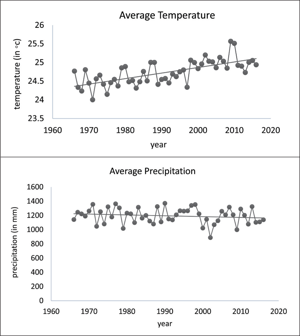
Projections indicate that climate change could severely affect global crop yields, with end-of-century losses estimated for wheat (9–12 per cent), corn (5.6–6.3 per cent), rice (18.1–19.4 per cent) and soyabeans (15.1–16.1 per cent) (Cui, 2020; Hussain et al., 2020). In India, alterations in temperature and precipitation regimes are anticipated to have profound implications for agricultural productivity. Over the past five decades, temperatures have exhibited a persistent upward trajectory, while long-term precipitation trends have remained relatively stable, though marked by notable interannual variability (see Figure 1). These trends could reduce rice and wheat yields by 8.1 per cent and 6.51 per cent by 2080, respectively (Wang et al., 2022). Rising temperatures may disrupt crop growth, intensify water stress, and heighten pest and disease pressures. Although precipitation remains stable, it may not offset these effects, especially as rainfall during the rice-growing season has declined by 7 per cent in the last 30 years (Daloz et al., 2021). Without adaptation, rain-fed rice yields could fall by 20 per cent by 2050 and by 47 per cent by 2080, while irrigated rice may see declines of 3.5 per cent and 5 per cent (Wang et al., 2018). Understanding these impacts necessitates examining both climatic and non-climatic factors, as temperature and rainfall directly influence crop productivity (Anderson et al., 2020; Aryal et al., 2020; Kumar & Sharma, 2022).

Figure 1.

Source: Authors’ analysis based on CMIE (2024) data.

Changes in temperature and precipitation, along with shifts in evapotranspiration and wind speed, have altered agro-ecological zones, affecting cereals, pulses, oilseeds and cash crops (Meena et al., 2015). In some cases, crop responses vary widely; for instance, rice yields rise by 5.21 per cent with increased rainfall but drop with higher wind and evapotranspiration; bajra benefits from temperature rise but declines with evapotranspiration; chickpea, groundnut and sugarcane also show similar sensitivities (Mohapatra et al., 2022). While most research centres on staples like rice and wheat, according greater attention to pulses, oilseeds and cash crops is vital for India’s food security, economic stability and rural livelihoods. A broader focus is essential to address the future implications of climate change across this wide array of crops through inclusive and targeted adaptation strategies.

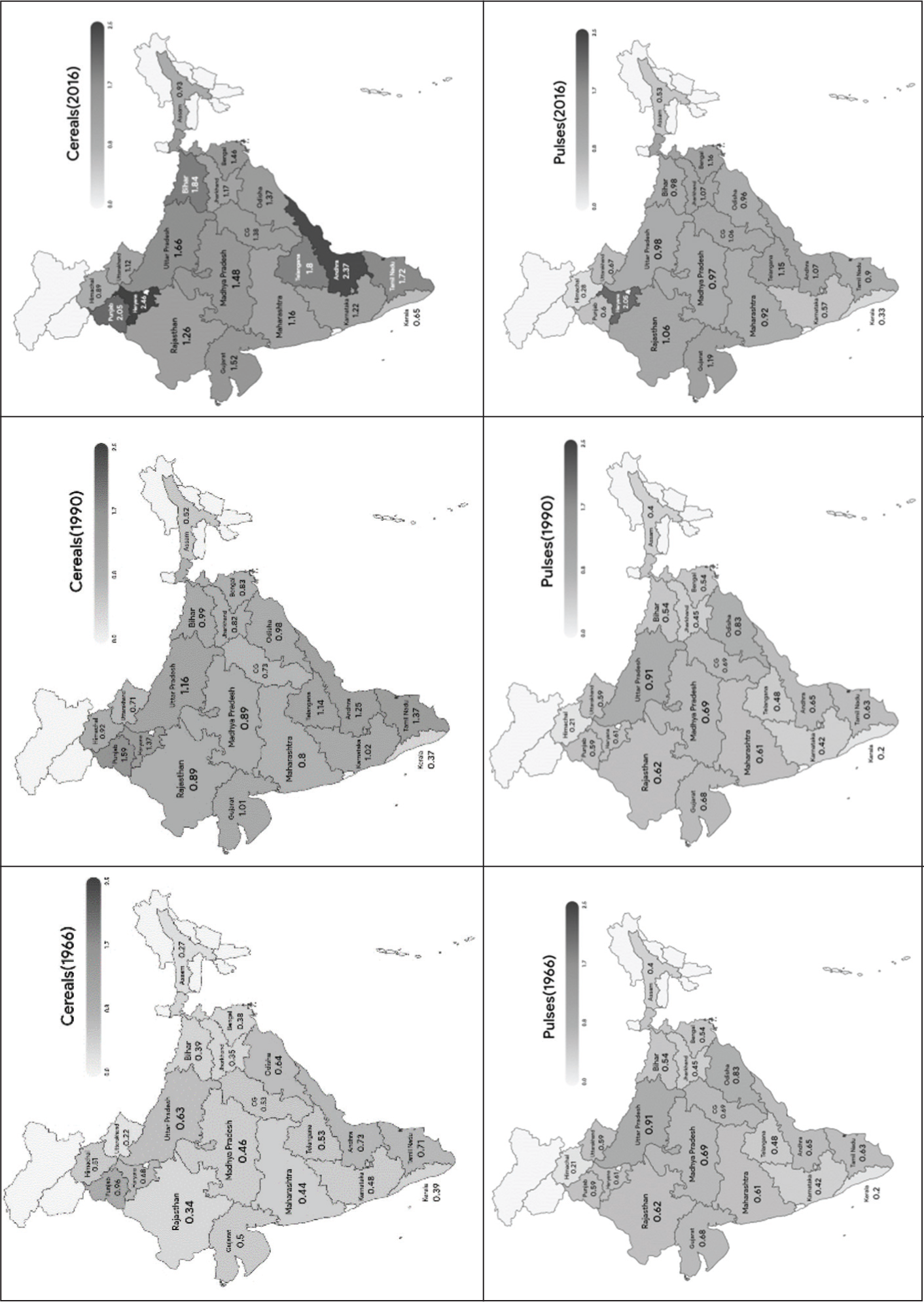
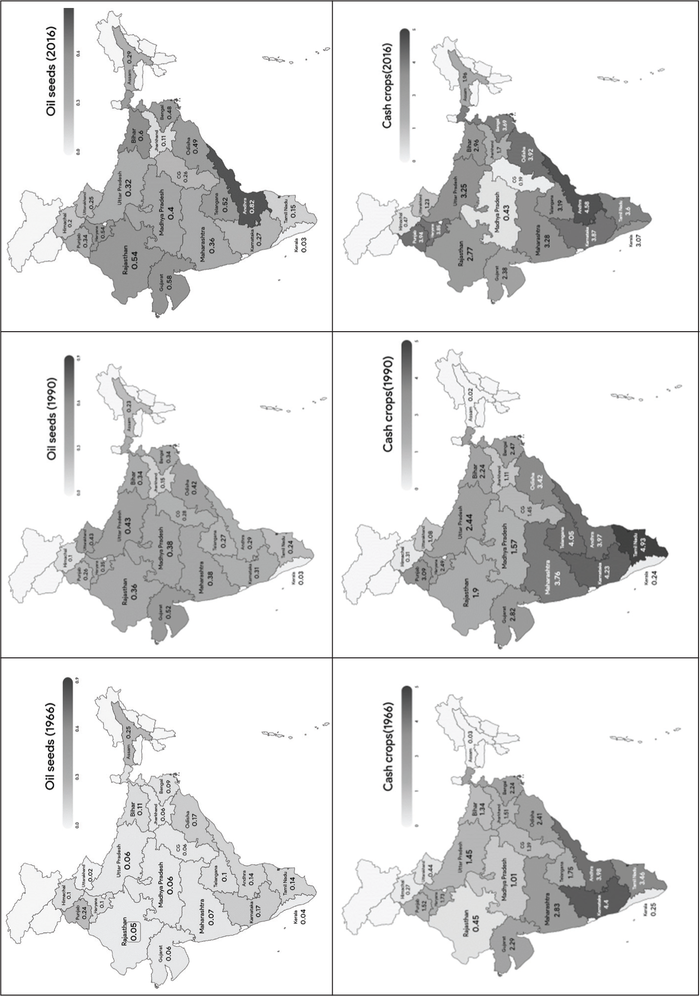
Agricultural reforms in the 1990s, supported by better access to advanced seeds, fertilisers and financial resources, significantly improved crop yields across India. These policy reforms led to major increases in cereal production in northern India and oilseed output in the south (see Figure 2).¹ Key inputs like improved seeds, irrigation and mechanisation played a critical role in boosting productivity and reducing labour dependence (Gulati & Juneja, 2020). These input-driven gains contributed to nationwide agricultural growth (Nadkarni, 2022). However, the long-term sustainability of these gains remains uncertain, highlighting the need to understand how agricultural inputs interact with climate variability and external stresses.

Figure 2.

Source: Authors’ analysis based on ICRISAT (2024) data.

Many studies examining the intersection of climate change and agriculture rely on temporal scopes of less than 30 years. While these shorter time frames effectively capture near-term climate variability and extreme weather events, they often miss the cumulative effects of gradual climate change on agronomic systems. For instance, Chen and Gong’s (2021) 35-year panel study, Chandio et al.’s (2020) 32-year analysis and Da et al. (2024) offer valuable insights into adaptation patterns, yet remain limited in capturing long-duration climatic shifts. Extending the temporal scale of analysis is vital to uncover long-term resilience thresholds and adaptive mechanisms as agricultural systems confront escalating climate risks.

India’s pivotal role in global food security underscores the importance of understanding how climate change affects its agricultural productivity. With the global population projected to reach 11 billion by 2100, sustaining food supply is crucial (Patel et al., 2020). Under high-emissions scenarios like SSP5-8.5, monsoon rainfall could increase by 24.3 per cent; around 0.33 mm/day or 5.3 per cent per °C of warming by the end of the century (Katzenberger et al., 2021; Yadav et al., 2024). These shifts may severely disrupt rice and wheat yields (Cui & Xie, 2022). To ensure resilience, it is equally vital to assess climate impacts on pulses and oilseeds, which are critical for dietary diversity and nutritional security.

Projected climatic changes in India include temperature increases of 2.3°C–3.9°C and rainfall gains between 61.5 mm and 98.2 mm by the 2080s. Eastern regions may see even sharper changes, with temperature rises of 2°C–4°C and rainfall increasing by up to 15 per cent, while coastal areas could face wind speed reductions of about 1 m/s (Karmacharya et al., 2017; Mishra et al., 2022). This regional variability necessitates adaptive strategies tailored to India’s diverse agro-ecological zones. Our study builds on these insights by integrating Intergovernmental Panel on Climate Change (IPCC) projections across multiple Shared Socioeconomic Pathways (SSP1-2.6 to SSP5-8.5), offering forward-looking analysis of crop productivity in India. While earlier studies, such as Choudhary et al. (2020), have analysed climate impacts on staple crop yields using extensive historical data over six decades, they have largely overlooked forward-looking projections that consider evolving climate scenarios. By bridging this gap, our study offers a critical framework to aid policymakers and stakeholders in anticipating and mitigating risks to agricultural productivity under future climate conditions, addressing both current impacts and long-term adaptation needs.

This research advances existing literature by addressing several key gaps. First, it undertakes a longitudinal analysis of crop–climate interactions using a panel dataset that spans 50 years (1966–2016), a period marked by profound transitions in Indian agriculture, including the Green Revolution, successive policy shifts and technological innovations. This extended time frame enables a robust assessment of how crop yields have responded to both climatic variability and non-climatic pressures over time. Second, the study expands the scope of prior research by including a diverse set of crops across four major categories, such as cereals, pulses, oilseeds and cash crops, many of which are typically overlooked in empirical assessments. This broad coverage allows for a detailed examination of heterogeneous crop responses to climate change, offering comparative insights that are essential for designing targeted adaptation strategies. Third, the analysis integrates forward-looking yield projections based on SSP climate scenarios, thereby providing a future-oriented perspective on the potential impacts of climate change on Indian agriculture. Fourth, the study employs advanced econometric techniques, including non-linear panel regression models, to address methodological challenges such as endogeneity, omitted variable bias and heterogeneity in crop response functions. Finally, by identifying empirically grounded yield thresholds, the research offers crop-specific and policy-relevant adaptation strategies that can inform agricultural planning and resilience-building efforts in a changing climate.

The structure of the paper is as follows. After the introductory Section 1, Section 2 outlines the theoretical background of the study. Section 3 details the data sources and the empirical methods used for the analysis. Section 4 presents the results and discussion, while Section 5 concludes with policy implications.

2. Theoretical Framework

To analyse the impact of climate change on Indian agricultural crops, this study conceptualises agricultural production through a weather-augmented framework where climatic variables act as environmental efficiency shifters, where the crop yield Y_it for state i at time t is determined by a vector of non-climatic inputs X_it and a set of climatic variables W_mit. Unlike conventional inputs that typically exhibit monotonic returns, environmental variables such as temperature and rainfall follow a non-linear pattern, contributing to productivity up to an optimal threshold before becoming detrimental. To capture this multiplicative relationship where climate scales the effectiveness of all other inputs, we model the production function using an exponential specification. In this framework, the production function is defined as follows:

Y_{i t} = \exp (α) \cdot \exp (X_{i t} \emptyset) \cdot \exp (Ω_{i t}) .

(1)

Here, the term exp(a) captures the Total Factor Productivity (TFP) characterised by constant returns to scale, while exp(X_itØ) represents the contribution of non-weather control variables X_it. The coefficients Ø represent the semi-elasticities, indicating that a one-unit change in non-climatic inputs results in a proportional percentage change in output. The term X_it represents the net environmental efficiency derived from climatic conditions. To account for the non-linear impacts of weather, we specify X_it as a quadratic function of the m weather variables.

Ω_{i t} = \sum (γ_{m} W_{m i t} + θ_{m} W_{m i t}^{2}) .

(2)

The coefficients γ_m and θ_m capture the linear and quadratic effects of the mth weather variable, respectively. This form allows the marginal effect of the weather variable W_mit to vary with its intensity, capturing both the beneficial and adverse deviations from ideal conditions.

By taking the natural logarithm of this production function, we derive the semi-logarithmic specification employed in our empirical analysis. The resulting equation is

\ln (Y_{i t}) = α + \emptyset X_{i t} + \sum (γ_{m} W_{m i t} + θ_{m} W_{m i t}^{2}) + ϵ_{i t} .

(3)

Equation (3) corresponds directly to Equation (6) in Section 3. Furthermore, the inclusion of the idiosyncratic error ε_it and unobserved random variables u_it [as detailed in Equation (7)] accounts for stochastic shocks to production, ensuring that the theoretical model is fully consistent with the econometric strategy of minimising bias from unobserved heterogeneity.

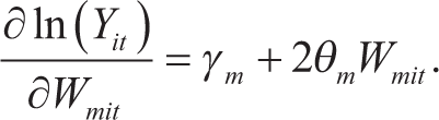
To further elaborate the relationship between climate and yield, we examine the marginal impact of climatic variables. The marginal effect of a specific weather variable W_mit on the log of crop yield is given by the partial derivative with respect to W_mit:

\frac{\partial \ln (Y_{i t})}{\partial W_{m i t}} = γ_{m} + 2 θ_{m} W_{m i t} .

(4)

Equation (4) underscores that the impact of climate is not constant but depends on the current level of the weather variable. We anticipate a concave relationship where θ_m < 0, indicating that the marginal benefits of weather variables diminish as they increase. This allows us to identify the optimal climatic condition, or ‘inflection point’, where yield is maximised. By setting the marginal effect to zero, we can solve for the optimal level of the weather variable W*_mit:

W_{m i t}^{*} = - \frac{γ_{m}}{2 θ_{m}}

(5)

Values of W_mit below this threshold indicate that increases in the weather variable are beneficial, while values above it suggest that further increases lead to yield losses.

3. Materials and Methods

3.1 Data Sources

This study utilises a longitudinal dataset covering a 50-year period from 1966 to 2016, drawing on ICRISAT (2024) data from 20 major agricultural states in India that collectively represent the principal contributors to national food grain production. The analysis focuses on 20 key crops, which are categorised into cereals, pulses, oilseeds and cash crops (see Appendix B, Table B1). In order to ensure data consistency and suitability for analysis, comprehensive data cleaning techniques were employed, resulting in a balanced panel dataset. This preparation is essential for conducting robust panel regression analysis and deriving reliable empirical insights.

Climatic variables, including temperature, precipitation, wind speed and evapotranspiration, were sourced from the Centre for Monitoring Indian Economy (CMIE, 2024), which provides consistent annual state-level data. Non-climatic variables, such as irrigation coverage, mechanisation and fertiliser use, were obtained from crop-specific data available through ICRISAT (2024). Since crop-wise fertiliser consumption data are not directly available, estimates were derived by prorating total fertiliser use across crops in accordance with their respective shares of cultivated area, following the method employed by Verma et al. (2020). In the absence of crop-disaggregated labour data, total agricultural labour in each state was proportionally allocated across crops based on their cultivated area. Data on electric pump sets and tractors were sourced from ICRISAT VDSA’s (2024) agricultural census. Due to the lack of crop-specific information for these inputs, the same proportional distribution method was applied, in line with the strategies adopted by Gupta et al. (2014), Padakandla (2016) and Mohapatra et al. (2022). This comprehensive methodological approach ensures consistency in estimating crop-level input intensities across states and over time.

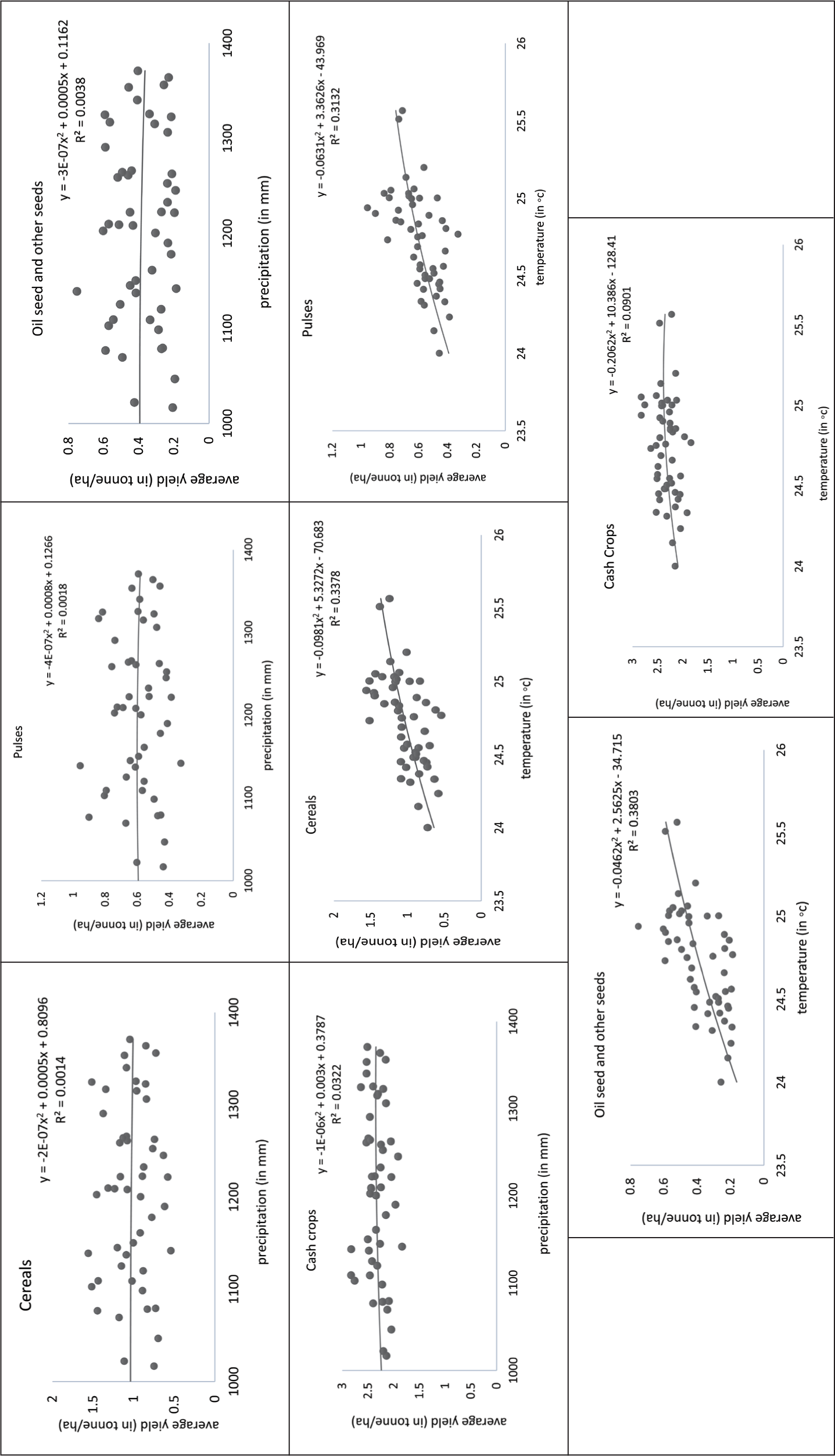
Scatter plot analysis confirms a non-linear relationship between crop yields and various climate variables,² revealing a possible quadratic association, as shown in Figure 3. While certain climate variables show strong correlations with yields, the relationship remains non-linear. For this study, two primary climate variables, temperature and precipitation, are emphasised, as these will serve as the basis for projecting crop yields under future climate scenarios.

Figure 3.

Source: Authors’ own work.

3.2 Empirical Methodology

This study employs a semi-log production function due to its econometric tractability and interpretability in capturing percentage changes in output. The functional form for state θ and time t is represented as: y_it = f(X_it, W_it). After accounting for all variables, the production function becomes

\ln Y_{i t} = α + \emptyset_{j} X_{j i t} + \sum_{m} (γ_{m} W_{m i t} + θ_{m} W_{m i t}^{2}) + δ_{t} + τ_{i} t + ε_{i t} .

(6)

Here, α captures the intercept in a production function characterised by constant returns to scale, implying linearity and homogeneity of degree one. Y_it represents the total crop yield for state i at time t. X_jit are non-weather control variables, coefficient Ø_j are semi-elasticities; a one-unit change in X_jit implies an approximate 100 Ø_j per cent change in Y_it. W_mit are weather variables (e.g., temperature and rainfall), γ_m and θ_m capture the linear and quadratic effects of the mth weather variable, allowing non-linear responses. d_t are year fixed effects, x_it are state-specific linear time trends, and f_it is the idiosyncratic error. The analysis applies crop-specific regressions to capture the nuanced responses to climatic and non-climatic factors.

The adoption of the semi-log functional form, as indicated by Sargan’s criteria (see Appendix B, Table B3), rejected the null hypothesis, supporting this structure’s necessity (see Appendix A, Note A1 for more details). We analyse the relationship between crop yield and both weather and non-weather factors using panel regression models, with several pre-estimation tests to ensure model robustness. The Fisher unit-root test (see Table B2) confirmed variable stationarity, while the Variance Inflation Factor (VIF) test (see Table B5) ruled out multicollinearity concerns.

To address unobserved random variables like farm inputs, denoted as γ, the regression equation is further expressed as (see Note A2):

l n (y_{i t}) = α + β x_{i t} + c .

(7)

However, applying the Ordinary Least Squares (OLS) method leads to bias and inconsistency in the βˆ estimator, as f(x, c) ≠ 0, indicating a correlation between unobserved variables and independent variables. The Hausman test suggests that γ follows a random effects pattern across states, ruling out the pooled OLS method. Additionally, the Pesaran test (see Table B4) confirmed significant cross-sectional dependence, while the Wooldridge test identified first-order autocorrelation, indicating both cross-sectional and serial autocorrelation across models (see Note A3).

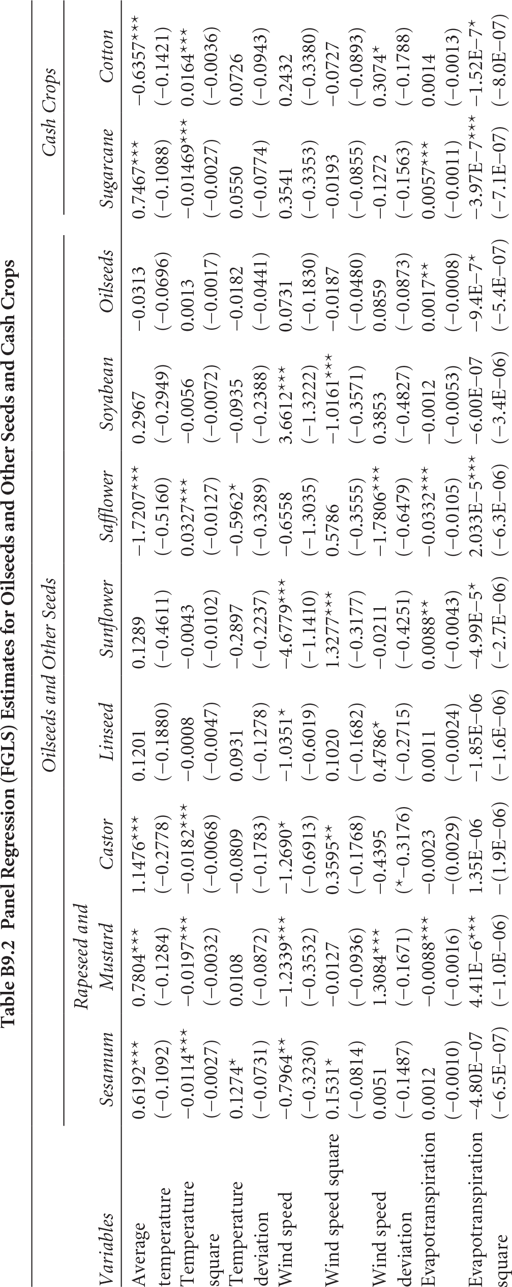
Although the Feasible Generalised Least Squares (FGLS) method is widely used for addressing serial correlation and cross-sectional dependence, it is often limited in accurately capturing heteroscedasticity in crop-specific regressions (see Table B9). In contrast, the Beck–Katz estimator, which employs Panel Corrected Standard Errors (PCSE), is more effective in adjusting for these issues without transforming the original data structure. PCSE provides consistent and reliable standard error estimates, particularly in datasets with a large number of cross-sectional units and relatively short time dimensions. As highlighted by Famanta et al. (2024), PCSE offers greater efficiency and accuracy in estimating model parameters in such cases, making it more suitable than FGLS for robust inference. Accordingly, the final model adopts the PCSE methods and is structured as follows:

Y_{i t} = X_{i t} β + ϵ_{i t} .

(8)

In this context, i indicates the total number of panels, while t corresponds to the time frame of the study within each panel. The symbol ε refers to the idiosyncratic error term, which may exhibit autocorrelation over time (t) or contemporaneous correlation across panels (i).

\begin{matrix} y_{1} \\ y_{2} \\ \begin{matrix} ⋮ \\ y_{n} \end{matrix} \end{matrix} = \begin{matrix} x_{1} \\ x_{2} \\ \begin{matrix} ⋮ \\ x_{n} \end{matrix} \end{matrix} β + \begin{matrix} ϵ_{1} \\ ϵ_{2} \\ \begin{matrix} ⋮ \\ ϵ_{n} \end{matrix} \end{matrix} .

The error covariance matrix Ω_NT is structured as Ω_NT = ΣX π:

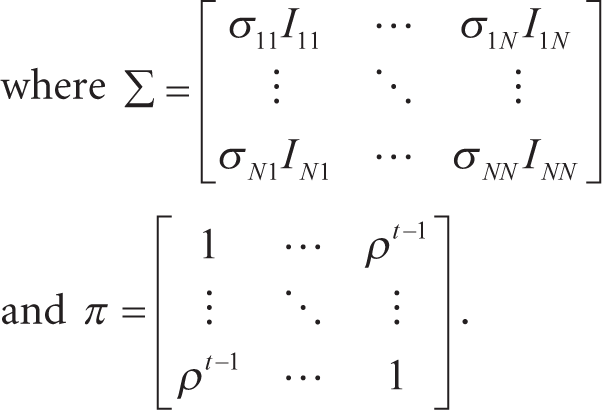
\begin{array}{l} w h e r e \sum^{​} = [\begin{matrix} σ_{11} I_{11} & \dots & σ_{1 N} I_{1 N} \\ ⋮ & ⋱ & ⋮ \\ σ_{N 1} I_{N 1} & \dots & σ_{N N} I_{N N} \end{matrix}] \\ a n d π = [\begin{matrix} 1 & \dots & ρ^{t - 1} \\ ⋮ & ⋱ & ⋮ \\ ρ^{t - 1} & \dots & 1 \end{matrix}] \end{array}

Here, Σ is the error covariance matrix and π is a temporal correlation matrix.

The PCSE estimator is computed as follows:

{\hat{β}}_{P C S E} = {({\tilde{x}}^{'} x)}^{- 1} {\tilde{x}}^{'} \tilde{y}

Cov ({\hat{β}}_{P C S E}) = {({\tilde{x}}^{'} x)}^{- 1} {\tilde{(x}}^{'} \sum \tilde{x}) {({\tilde{x}}^{'} x)}^{- 1}

Here, x~ and y~ represent the Prais-transformed observations of the explanatory and dependent variables, respectively. The PCSE method accounts for both cross-sectional dependence and serial autocorrelation, making it well-suited for our analysis of crop yields. The PCSE estimator for the covariance matrix is ${\hat{Σ}}_{i t} = \frac{ϵ_{i}^{'} ϵ_{t}}{T_{i t}},$ where ε'_i and ε_t are residuals for panels i and t, and T_it is the number of matched residuals by time period. In balanced panels, where all periods are common, T_it = T, representing the number of observations per panel.

In this study, we applied PCSE regression to account for both cross-sectional dependence and serial autocorrelation, resulting in more reliable forecasts of future crop yields under changing climate conditions. To assess the marginal effects of climatic variables such as temperature and precipitation, we calculate partial derivatives based on the estimated panel regression coefficients. The net impact of these weather variables on crop yield is derived by summing their respective marginal effects. The equation for this marginal effect is expressed as follows:

\frac{\partial l n Y_{i t}}{\partial W_{m i t}} = γ_{m} + 2 θ_{m} W_{m i t} .

(9)

(See Appendix A, Note A4 for more details.)

To assess crop tolerance under different climate scenarios, we determine the inflection points, thresholds beyond which further changes in weather may reduce yields. If θ_m ≠ 0; the turning point (value of W_mit that maximises/minimises lnY_it) is: $W_{m}^{*} = - \frac{γ_{m}}{2 θ_{m}}$

With the methodology established, Section 4 delves into the historical impacts of climate variables on crop yields in India, highlighting the effects across various crop categories, including cereals, pulses, oilseeds and cash crops.

4. Results and Discussion

The following three sub-sections present the empirical results. Section 4.1 examines historical climate impacts on crop yields, comparing climatic and non-climatic effects across crop categories. Section 4.2 explores future yield projections under alternative IPCC climate scenarios, analysing crop-specific responses to combined increases in temperature and precipitation over the twenty-first century. For robustness, Section 4.3 compares the estimation results from the FGLS and PCSE methods, respectively.

4.1 Historical Climate Effects on Crop Yields

4.1.1 Cereals

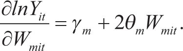
The elasticity analysis (see Appendix B, Table B8) for cereals highlights the complex interplay between yield, climate variables and non-climate factors. Temperature emerges as a major determinant, with rice and wheat exhibiting strong negative elasticities of −24.58 and −17.50, respectively, indicating that yield declines as temperatures rise. Wheat appears particularly vulnerable to heat stress, with a critical threshold at 17.63°C beyond which yields decrease sharply. This trend aligns with the study by Jyothsna et al. (2024), who report that high night temperatures (>25°C) can reduce rice yield by 10–15 per cent, while day temperatures (>35°C) can cause a 10–20 per cent decline due to increased respiratory losses. In contrast, pearl millet and finger millet show positive elasticities of 6.78 and 20.77, respectively, supporting their characterisation as climate-resilient, next-generation crops (Neupane et al., 2022). However, their squared terms reveal that the positive impact tapers off beyond certain thresholds.

Wind speed also significantly influences cereal yields, though effects vary across crops. Rice benefits from moderate wind, showing a positive elasticity of 6.50, possibly aiding pollination. In stark contrast, wheat is highly sensitive, displaying a sharp negative elasticity of −77.54, likely reflecting wind-induced physical damage. Sorghum appears more resilient (see Figure 4), though its squared term indicates a turning point at 2.05 m/s, beyond which wind becomes detrimental. This resilience strengthens the view of DeFries et al. (2023) that sorghum could be a climate-resilient substitute for wheat under future climate scenarios.

Figure 4.

Source: Authors’ own work.

The role of precipitation’s role is equally critical, especially when considering its interaction with irrigation. Rice shows a negative elasticity of −0.42, suggesting susceptibility to excess rainfall and related risks like waterlogging. However, Ashkra et al. (2023) find a positive link between rainfall and rice yield, indicating a 1.58 per cent increase in yield per additional millimetre of rainfall, highlighting the urgent need for temperature-tolerant, water-efficient rice varieties. Maize and sorghum, with positive elasticities of 0.0023 and 0.3197, respectively, thrive under increased rainfall, particularly in rain-fed regions. For finger millet, precipitation benefits decline beyond 1,000 mm.

Among the non-climate variables, fertiliser application positively affects yields across cereals, except in the case of wheat, highlighting the importance of nutrient inputs. Mechanisation, particularly tractor usage, strongly enhances rice and sorghum yields, with rice showing a regression coefficient of 5.99 (see Table B6). Irrigation infrastructure, reflected by electric pump set usage, also proves critical. Rural literacy shows mixed effects, likely boosting yields through better adoption of technology. However, labour elasticity varies, influenced by differing mechanisation levels. The spread of High-Yielding Varieties (HYVs) significantly improves yields, especially in the case of rice and pearl millet, underlining the essential role of improved seed technologies in strengthening climate resilience.

4.1.2 Pulses

Chickpea shows a modest positive temperature coefficient of 0.2305, suggesting a slight benefit from warmer conditions when only climate factors are considered (see Table B7). This positive effect grows significantly with the inclusion of non-climate variables, such as irrigation, where elasticity rises to 10.32. This finding aligns with the study by Neelima and Kumar (2023), who emphasise that technological advancements can enhance crop resilience to climate variability. However, Bera (2021) highlights that erratic rainfall and extreme weather introduce challenges for pulse production, such as delayed sowing and heat-stress-induced yield losses, potentially offsetting temperature-related gains.

For groundnut, higher temperatures initially result in a negative coefficient of −0.4200 under the climate-only model, indicating heat vulnerability. Yet, when non-climate factors are considered, elasticity becomes positive (23.06), suggesting that management practices can effectively mitigate temperature stresses. This supports the view of Gull et al. (2020), who found that pulses are highly sensitive to heat stress, particularly during flowering, though targeted interventions can help buffer some impacts.

Wind speed generally negatively affects pulse crops, with chickpea and pigeon pea showing strong negative elasticities of −51.51 and −58.24, respectively, likely due to physical damage or increased evapotranspiration. Groundnut is less affected (−26.92) but remains vulnerable. Precipitation initially benefits groundnut yields (0.00077), but when non-climate factors are introduced, the precipitation deviation coefficient shifts to −2.90E−04 (see Figure 5), suggesting that excess rainfall can become detrimental under compounding stressors.

Figure 5.

Source: Authors’ own work.

Other factors, such as rural literacy and agricultural labour availability, positively influence pulse yields, though minor pulses exhibit slight declines (−0.89), reflecting varying labour needs across pulse varieties.

4.1.3 Oilseeds and Other Seeds

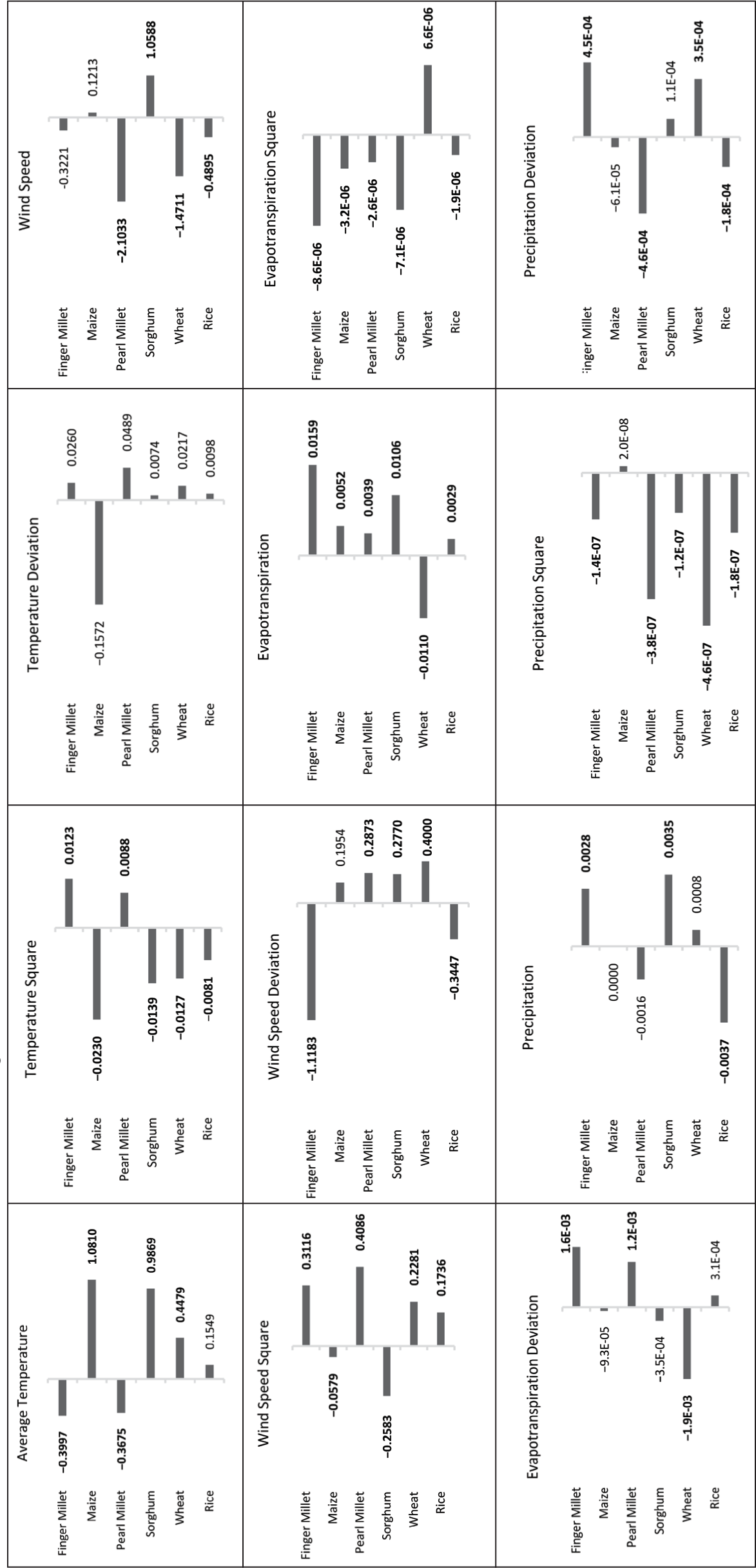
Temperature affects oilseed yields in diverse ways, underscoring the varied sensitivities of different crops to climatic changes. Castor shows a strong positive elasticity of 56.48, indicating its ability to thrive under warmer conditions, likely due to its adaptability and heat tolerance (see Appendix B, Table B8). In contrast, rapeseed and mustard, and linseed display negative elasticities of −6.68 and −7.61, respectively, suggesting that higher temperatures inhibit their productivity. The case of rapeseed and mustard is particularly noteworthy, as the significant negative square term of −0.0100 (see Figure 6) implies that temperatures exceeding an optimal 21°C lead to a sharp reduction in yields. These results align with Pillai and Walia (2024), who emphasise the heightened vulnerability of mustard to climate change, with both temperature and rainfall negatively impacting its resilience.

Figure 6.

Source: Authors’ own work.

Wind speed presents distinct challenges across oilseed varieties. Sesamum records a negative elasticity of −14.21, reflecting its sensitivity to high wind speeds that can elevate evapotranspiration and cause physical damage. Conversely, castor demonstrates a positive elasticity of 51.08, suggesting greater resilience, possibly due to its robust physiology or cultivation practices in more sheltered environments. Moreover, Maity et al. (2023) highlight that self-pollinated crops, such as several oilseeds, suffer greater yield reductions under temperature stress, indicating that wind may amplify yield variability.

Evapotranspiration further influences yields in complex ways. Sunflower exhibits a turning point at 828 mm, with an elasticity of −4.06 beyond this threshold, while safflower, despite a positive elasticity of 231.60, faces declining yields beyond 1,071 mm of evapotranspiration.

Precipitation effects are equally nuanced. Castor benefits from rainfall, showing a positive elasticity of 0.95, whereas sesamum and linseed respond negatively, with elasticities of −0.07 and −0.25, respectively. Notably, sesamum yields sharply decline beyond 1,759.25 mm of precipitation.

Socio-agronomic variables also play critical roles. Irrigation significantly boosts sesamum yields (elasticity 23.65), though excessive irrigation reduces rapeseed and mustard productivity (−19.48). Fertiliser use enhances safflower yields (elasticity 0.0110), highlighting the importance of nutrient management.

4.1.4 Cash Crops

Sugarcane and cotton display distinct sensitivities to temperature. For sugarcane, a 1 per cent increase in average temperature boosts yield by 7.01 per cent, indicating a strong positive response. Cotton similarly exhibits a positive elasticity of 7.65 per cent, though the effect tapers at higher temperatures, suggesting vulnerability to extreme heat. This pattern aligns with Jans et al. (2021), who project a 50 per cent increase in cotton output under RCP8.5 by 2,099, despite lower water availability due to CO₂-driven effects. Farooq et al. (2023) also warn that rising temperature and precipitation variability threaten the resilience of cotton.

Evapotranspiration similarly affects these crops in nuanced ways. For sugarcane, the positive influence of evapotranspiration declines beyond 782.05 mm, as indicated by negative squared terms (see Figure 7). Cotton’s critical threshold is higher, at 1,291.67 mm, after which further evapotranspiration reduces yields.

Figure 7.

Note: Significant results are in bold.

Precipitation presents a dual impact. Sugarcane benefits from rainfall up to 3,750 mm, beyond which yields decline, likely due to waterlogging or nutrient leaching. Cotton, conversely, shows a negative elasticity of −0.24 per cent, highlighting its sensitivity to excess moisture.

Non-climatic factors are equally crucial. Irrigation supports both sugarcane and cotton crops, though sugarcane experiences diminishing returns when combined with heavy rainfall. Cotton benefits from irrigation but requires careful moisture regulation. Mechanisation also shows contrasting effects: sugarcane yields fall with tractor use (elasticity of −121.74), while cotton gains significantly from mechanisation, with a positive elasticity of 1,009.17, reflecting its greater dependence on efficient mechanised practices.

4.2 Future Climate Scenarios

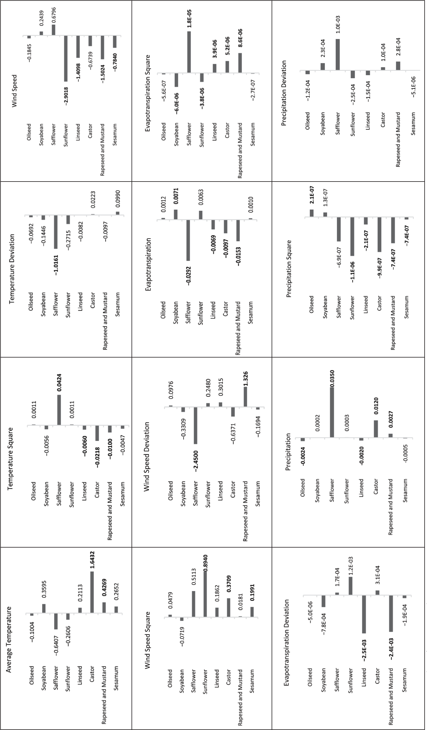
To analyse the future projections of crop yields under climate change scenarios, we use findings from SSP1-2.6 for precipitation and SSP5-8.5 for temperature across three periods: 2021–2040, 2041–2060 and 2081–2100 (see Figure 8).³ These projections highlight varying levels of crop resilience and sensitivity to climatic changes, revealing both adverse and favourable trends.

Figure 8.

Source: Authors’ own work.

Among cereals, wheat is the most negatively impacted, with yield losses increasing from 18.74 per cent to 27.35 per cent by the end of the century. This sharp decline is consistent with Daloz et al. (2021), who reported wheat yield reductions ranging from 4 per cent to 36 per cent under rising temperatures and reduced irrigation. In contrast, pearl millet displays resilience, with projected yield gains ranging from 17.99 per cent to 24.09 per cent, suggesting its adaptability under warming and erratic rainfall conditions. Rice experiences moderate yield reductions between −3.51 per cent and −8.71 per cent, particularly in later periods, supporting Singh et al. (2024), who found similar declines in rice yields in Uttar Pradesh under comparable SSP scenarios. Maize exhibits significant vulnerability, with yields falling from −12.78 per cent to −28.44 per cent, highlighting its sensitivity to temperature extremes. Conversely, finger millet performs better, with projected yield gains increasing from 12.57 per cent to 20.78 per cent. These contrasts suggest that future climatic conditions may favour pearl millet and finger millet while posing challenges for wheat, rice and maize cultivation.

The pulses group shows mixed outcomes. Pigeon pea is highly vulnerable, with yields declining steeply from −15.09 per cent to −33.51 per cent, reflecting its pronounced sensitivity to temperature rises as observed by Bera (2021). Chickpea also records negative trends, with yield reductions ranging from −4.22 per cent to −11.18 per cent, indicating its susceptibility to heat stress and reduced water availability. However, groundnut presents a strong positive response, with projected yield improvements ranging from 29.17 per cent to 38.04 per cent. This finding aligns with the study by Kadiyala et al. (2021), who reported similar yield gains under a conductive climate effect, highlighting the greater adaptability of groundnut relative to other pulses.

Among oilseeds, rapeseed and mustard display consistent yield reductions, worsening from −11.38 per cent to −18.22 per cent, due to temperature-induced damage to flowering and seed-setting processes. Soyabean shows moderate resilience, with slight yield declines from 5.14 per cent to 1.31 per cent, suggesting a potential plateau under future climates. In contrast, safflower exhibits strong positive projections, with yield gains rising from 9.64 per cent to 36.47 per cent, pointing to its robust adaptability to higher temperatures.

Cash crops exhibit diverse patterns. Cotton demonstrates substantial yield improvements, increasing from 21.58 per cent to 31.78 per cent, consistent with Jans et al. (2021), who projected a 50 per cent rise in cotton production under RCP8.5 by 2,099. The heat tolerance and lower water demands of cotton likely explain this positive trend. In contrast, sugarcane faces yield reductions ranging from −4.37 per cent to −15.48 per cent, reflecting its vulnerability to increased temperature and precipitation variability.

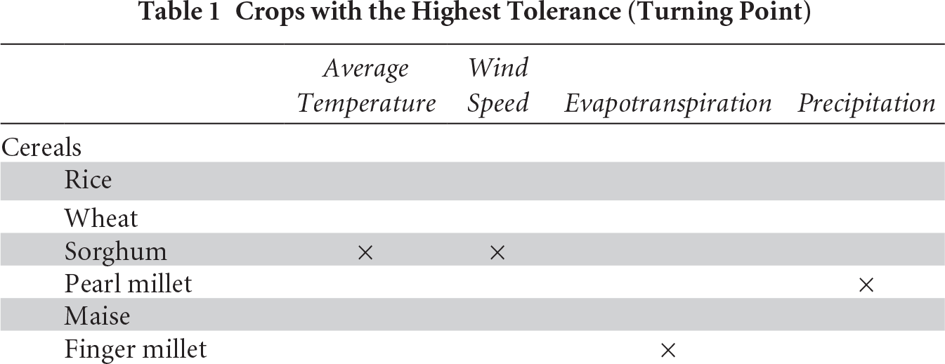
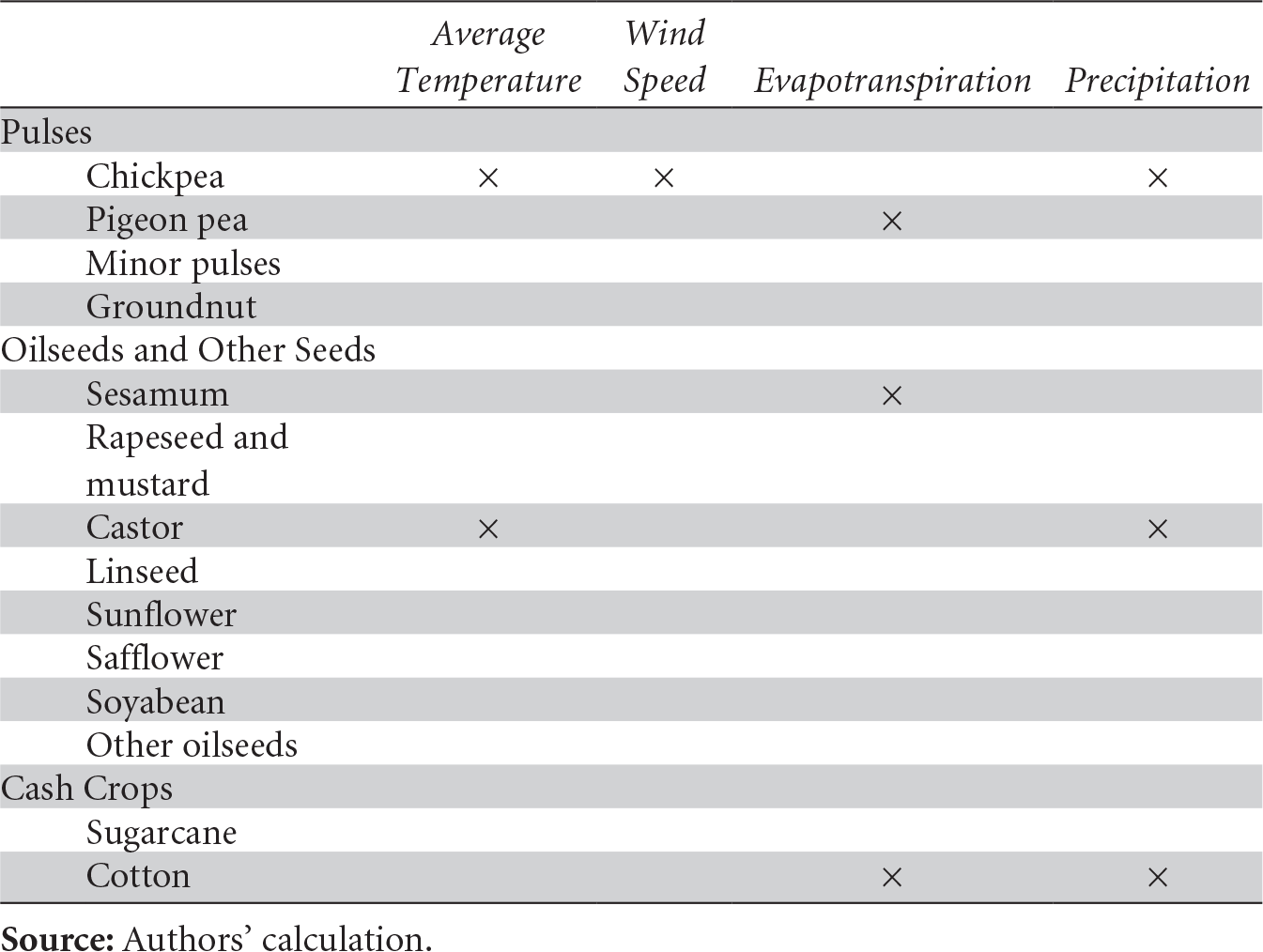
Overall, future projections indicate that climate change will significantly reshape Indian agriculture. Wheat, pigeon pea and sugarcane emerge as among the most adversely affected crops, while groundnut, safflower and cotton show notable yield gains; these trends are further elucidated in Table 1, which highlights the specific thermal thresholds that dictate these varying outcomes. These outcomes underscore the urgent need for crop-specific adaptive strategies, focusing on the promotion of climate-resilient varieties and the development of targeted interventions to support the most vulnerable crops.

Table 1.

Crops with the Highest Tolerance (Turning Point)

		Average Temperature	Wind Speed	Evapotranspiration	Precipitation
Cereals
	Rice
	Wheat
	Sorghum	×	×
	Pearl millet				×
	Maise
	Finger millet			×
Pulses
	Chickpea	×	×		×
	Pigeon pea			×
	Minor pulses
	Groundnut
Oilseeds and Other Seeds
	Sesamum			×
	Rapeseed and mustard
	Castor	×			×
	Linseed
	Sunflower
	Safflower
	Soyabean
	Other oilseeds
Cash Crops
	Sugarcane
	Cotton			×	×

Source: Authors’ calculation.

4.3 Robustness Check

A comparative analysis between FGLS and PCSE reveals substantial alignment in the direction of effects but divergence in coefficient magnitudes and levels of statistical significance, highlighting PCSE’s relative robustness in estimating climate–crop yield relationships. Both estimators confirm the positive and significant impact of temperature on heat-tolerant crops, with PCSE yielding coefficients of 0.4479 for wheat, 0.9869 for sorghum and 1.3850 for pigeon pea, all significant. FGLS likewise reports significant effects, with somewhat smaller magnitudes: 0.6050, 0.6173 and 1.2514, respectively. For the concave temperature–yield relationship in wheat, both models detect significant negative effects, with PCSE estimating −0.0127 and FGLS being slightly steeper at −0.0159. However, differences emerge in the influence of precipitation; PCSE reports a significant negative effect on rice (−0.0037), capturing waterlogging sensitivity, while FGLS presents a non-significant, near-zero estimate (0.0006). As regards wind speed, PCSE indicates a strongly significant and large negative impact on rapeseed (−1.5024), whereas FGLS also identifies a significant but slightly lower effect (−1.2339). Turning to agricultural inputs like fertiliser, FGLS reports highly significant but inflated impacts, such as 1.1118 for rice and 1.6905 for maize, whereas PCSE provides more measured yet significant estimates: 0.1765 and 1.9184, respectively. Mechanisation proxies like electric pumps and tractors are also significant in PCSE but again appear exaggerated under FGLS. Overall, PCSE not only retains statistical significance across critical variables but does so with coefficient sizes that align more closely with field-level dynamics, making it the more dependable estimator for climate impact studies and policy-oriented agricultural analysis.

5. Conclusion and Policy Implication

This study offers a novel and rigorous assessment of climate change impacts on Indian agriculture by examining crop-specific yield responses across a 50-year panel (1966–2016), capturing a period of significant agricultural transformation driven by policy shifts and technological change. Unlike prior research by Gupta et al. (2014), Burke and Emerick (2016) and Chen and Gong (2021), which focused on aggregated crop groups or shorter time frames, this analysis disaggregates yields across four major crop categories such as cereals, pulses, oilseeds and cash crops, allowing for a more comprehensive and differentiated understanding of climatic and non-climatic influences on productivity. The extended temporal coverage strengthens the reliability of long-run crop–climate interaction estimates, while the broader crop selection moves beyond conventional staples, addressing gaps in existing literature. A key novelty lies in the integration of forward-looking projections using Shared Socioeconomic Pathways (SSP 1–2.6 for precipitation and SSP 5–8.5 for temperature), which reflect both mitigation-aligned and high-impact climate trajectories. These projections are combined with non-linear estimation techniques to identify crop-specific yield inflection points for temperature and precipitation, offering insights into critical thresholds where climate stress may trigger disproportionate yield losses. The adoption of advanced econometric methods further ensures robust estimation by addressing issues of heteroscedasticity, autocorrelation and cross-sectional dependence. Overall, the methodological design and empirical depth of the study signify an original contribution to the literature, generating policy-relevant evidence to inform adaptive strategies tailored to crop-specific climate sensitivities.

The research identifies key vulnerabilities and adaptive capacities across major crop groups in response to climate variability, noting that staple cereals like rice, wheat and millet face substantial risks from temperature fluctuations and shifting precipitation patterns, which threaten India’s food security. Water-intensive crops like rice, central to Indian diets, are especially susceptible to yield reductions in water-stressed areas, whereas drought-tolerant cereals like pearl millet and finger millet demonstrate resilience, making them viable substitutes in drought-prone regions. The study recommends the implementation of improved irrigation methods, such as drip and micro-irrigation, and rainwater harvesting to stabilise cereal yields in vulnerable areas (Di Falco & Chavas, 2006). Pulses, particularly chickpeas and groundnuts, exhibit heightened sensitivity to rising temperatures and rainfall variability, emphasising the need for diversification, wherein heat-tolerant crops like chickpea could be alternatives in warmer regions (Jaworski et al., 2023). Soil conservation practices like mulching, no-till farming and bio-fertiliser integration are recommended to bolster the resilience of pulse crops by enhancing soil moisture retention and quality.

As regards oilseeds, soyabean and sunflower emerge as relatively resilient under moderate climate fluctuations, making them suitable for regions experiencing increased variability. The study suggests enhancing irrigation efficiency through the adoption of sub-surface methods and promoting rainwater harvesting infrastructure to support yield stability for these crops even during dry spells. Cash crops like sugarcane and cotton, with high water demands, face intensified risks under climate stress; thus, introducing drought-tolerant varieties and practices like crop rotation and intercropping can help mitigate these vulnerabilities, while enhancing long-term productivity (Da Cruz & Machado, 2023; Okemo et al., 2024). To mitigate food security risks and advance agricultural sustainability, policies should focus on adopting climate-smart agricultural technologies, including advanced breeding, improved irrigation and soil management techniques to increase crop resilience against extreme weather. By diversifying crop production and emphasising sustainable water use, India can reinforce agricultural stability amidst climate change, safeguarding both rural livelihoods and national food security.

Despite its strengths, this study has certain limitations. The CMIE and IndiaStat databases, while comprehensive, have limitations in crop-specific data for variables such as agricultural labour, mechanisation and fertiliser usage, which required us to rely on weighted estimates based on cropping area. While this approach provides a broad perspective, it may not fully capture resource allocation nuances across individual crops, introducing potential inaccuracies. Additionally, data on agricultural equipment use were available only at five-year intervals, necessitating extrapolation that may impact the analysis’s precision. Furthermore, we did not incorporate climate variables like soil moisture and radiation, given their limited availability and inconsistent measurements across states. While these variables are undoubtedly important, they were omitted to ensure robustness in longitudinal data.

Future research should take the next steps towards developing refined adaptation strategies, particularly by testing additional climate variables such as soil moisture, solar radiation and extreme weather events, which were limited in the current study due to data constraints. Comparative analyses of adaptation strategies between India and other developing nations with similar agro-ecological climates would also help identify globally applicable solutions. An interdisciplinary approach combining insights from agricultural science, environmental economics and climate modelling could improve our understanding of effective adaptation techniques. Such an approach, like evaluating the significance of crop genetic variety and innovative irrigation systems, could provide useful insights on enhancing resilience across various agro-ecological zones.

Footnotes

Acknowledgements

We thank the handling editor and anonymous reviewers for their constructive comments and suggestions that significantly improved the manuscript. An earlier version of this paper was presented at the 8^th SANEM Annual Economists’ Conference (21–23 February 2025, Dhaka). We are grateful to the participants at these events for their valuable feedback. Any remaining errors are our own.

Data Availability Statement

The data that support the findings of this study are available upon reasonable request from the corresponding author.

Declaration of Conflicting Interests

The authors declared no potential conflicts of interest with respect to the research, authorship and/or publication of this article.

Funding

The authors received no financial support for the research, authorship and/or publication of this article.

Permission to Reproduce Material from Other Sources

All materials included in this manuscript are original or used with appropriate permission and citation.

Appendix A: Notes

A1. For two models, say one is linear and the other in semi-log form, then Sagan’s criteria would prompt towards the best-fit model using the following expression: ∀ = [φ₁/g₂ φ₂]ⁿ, where φ₁ is the standard deviation of the combined residual (sum of random or fixed error component and overall stochastic error component) of Model 1; φ₂ is the standard deviation of the combined residual of Model 2; g₂ is the geometric mean of the dependent variable of Model 2, and n is the number of observations. If ∀ < 1, then Model 1 is favoured, and if ∀ > 1, then Model 2 is favoured.

A2. Assuming a linear model, where the focus is on the k × 1 vector β, which represents both climate and non-climate coefficients, if Cov (x, c) ≠ 0, then including ‘γ’ as the error term is inappropriate, and β cannot be estimated without additional information. The model with the error term is f_it.

\begin{array}{l} {\hat{β}}_{O L S} = \frac{{\sum^{​}}_{i = 1}^{n} {\sum^{​}}_{t = 1}^{t} x_{i t} y_{i t}}{{\sum^{​}}_{i = 1}^{n} {\sum^{​}}_{t = 1}^{t} x_{i t}^{2}}, \\ = \frac{{\sum^{​}}_{i = 1}^{n} {\sum^{​}}_{t = 1}^{t} x_{i t} (β x_{i t} + ε_{i t})}{{\sum^{​}}_{i = 1}^{n} {\sum^{​}}_{t = 1}^{t} x_{i t}^{2}}, \\ = β + \frac{{\sum^{​}}_{i = 1}^{n} {\sum^{​}}_{t = 1}^{t} x_{i t} (ε_{i t})}{{\sum^{​}}_{i = 1}^{n} {\sum^{​}}_{t = 1}^{t} x_{i t}^{2}} . \end{array}

The OLS βˆ estimator becomes biased and inconsistent because f (x, c) ≠ 0, as ‘γ’ is correlated with ‘x’, making pooled OLS inappropriate. Before applying the error correction panel model, it is important to discuss the nature of the unobserved effect so that the model is (A1)

Δ y_{i t} = Δ x_{i t} β + c_{i} + ε_{i t} .

A3. The null hypothesis of the Hausman test assumes random effect estimates are consistent and efficient. The Hausman test shows that ‘γ’ has a random effect across states, so a pooled OLS estimation of the unobserved effect model is used as $Δ y_{i t} = Δ x_{i t} β + ϑ_{i t} ,$ where $ϑ_{i t}$ = $c_{i} + ε_{i t}$ is the composite error (A2).

For pooled OLS to be consistent, the estimation of this equation requires as follows: (A3)

f (x_{i t} ​, ϑ_{i t}) = 0.

The expression for the test is given as

H = {({\hat{β}}_{F E} - β_{R E})}^{'} {[V_{F E} - V_{R E}]}^{- 1} (β_{F E} - β_{R E}) ~ χ^{2 (k)},

where ${\hat{β}}_{R E}$ and ${\hat{β}}_{F E}$ are the vectors of coefficient estimates for the random effects and fixed effects models, respectively, χ² represents chi-square, and the degree of freedom k represents the number of factors.

The initial model with y_it violates certain assumptions because y_{i, t –} ₁ and γ_i are correlated, while ϑ_it is serially correlated with γ_i across time periods (see Equation (A3)). This correlation highlights the need for more robust tests and a random effects analysis, as the model’s assumptions are no longer met. Specifically, we must impose stricter assumptions to ensure the robustness of the estimates, including the conditions of strict exogeneity and orthogonality between ϑ_it and x_it.

The assumptions required are:

E (\cup_{i t} | x_{i t} ​, c_{i}) = 0, E (c_{i} | x_{i t}) = E (c_{i}) = 0.

The random effects approach accounts for serial correlation in the composite error term, where ϑ_it = γ_i + U_it thus capturing spatial correlation as well. The suitable regression model for this set-up is expressed as (A4)

y_{i t} = x_{i t} β + U_{i t} .

Here, y_it is the observed crop yield for state ith in time period tth, while x_it is a vector of K × 1 observation on non-stochastic regressors and U_it is the regression disturbance, defined as (A5)

U_{i t} = μ + ϵ_{i t} ​,

(A6)

ϵ_{i t} = ρ ω + ϑ_{i t} .

In this case, μ = (μ₁,…, μ_N) represents the random state effects vector, assumed to be independently and identically distributed (IIN) with a variance of μ². The autoregressive coefficient t measures the degree of correlation, while W is an N × N weight matrix. Equation (A6) indicates that part of the current error depends on past errors, with ϑ_it representing the new disturbance or shock for the current period. This autoregressive nature of the error term is crucial in the model’s design. The error term ε_it is thus represented as

ϵ_{i t} = {(I_{N} - ρ W)}^{- 1} ϑ_{t} = B^{- 1} ϑ_{t} .

Hence, the full disturbance term U is expressed as

U = {(τ_{t} X I_{N})}_{μ} + {(I_{t} X B^{- 1})}_{ϑ} .

Now, under the assumption of normality, the likelihood function is $L = - N T / 2 l n 2 π σ^{2} ϑ - 1 / 2 l n | \sum | - 1 / 2 (σ^{2} ϑ) \overset{'}{U} \sum^{- 1} U,$ where U = y – xb is the error covariance matrix. The first-order conditions for maximum likelihood estimation (MLE) and the Lagrange Multiplier (LM) test for m = 0 are derived for this model.

A4. Marginal effect of temperature: $\frac{\partial}{\partial y} l n y \frac{\partial y}{\partial T e m p} = φ_{1} + 2 φ_{2} T e m p + φ_{7} P r e c p$ (24)

Or \frac{\partial y}{\partial T e m p} = (φ_{1} + 2 φ_{2} T e m p + φ_{7} P r e c p) y .

Marginal effect of precipitation: $\frac{\partial}{\partial y} l n y \frac{\partial y}{\partial P r e c p} = φ_{4} + 2 φ_{5} P r e c p + φ_{7} T e m p$

Or \frac{\partial y}{\partial P r e c p} = (φ_{4} + 2 φ_{5} P r e c p + φ_{7} T e m p) y .

Here, y denotes crop yield (tonne/ha), φ s are the regression coefficients associated with the weather variable, its quadratic terms, and φ₇ is the regression coefficients of the intersection terms between temperature and precipitation, respectively. Using y = 100 as the baseline, we compute the effects of marginal increases in weather parameters.

The total effect on crop yield is the sum of the marginal effects of temperature and precipitation. Additionally, we calculate the elasticity of crop yield in response to weather variables using the following equation: $\frac{\partial y}{\partial W} = (φ_{1} + 2 φ_{2} W) y$ and for non-weather variables: $\frac{\partial y}{\partial X} = (φ_{i}) y .$

Appendix B: Tables

Table B9.2

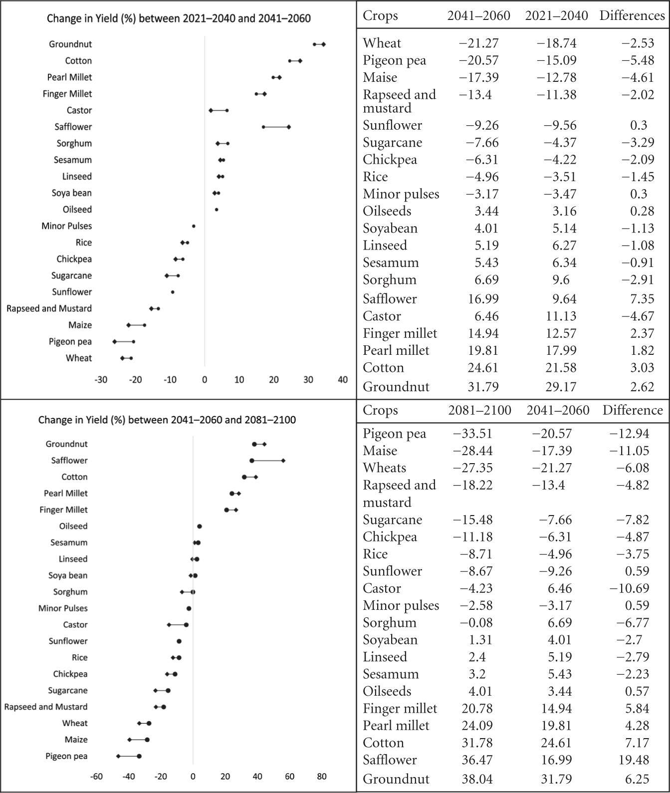
Panel Regression (FGLS) Estimates for Oilseeds and Other Seeds and Cash Crops

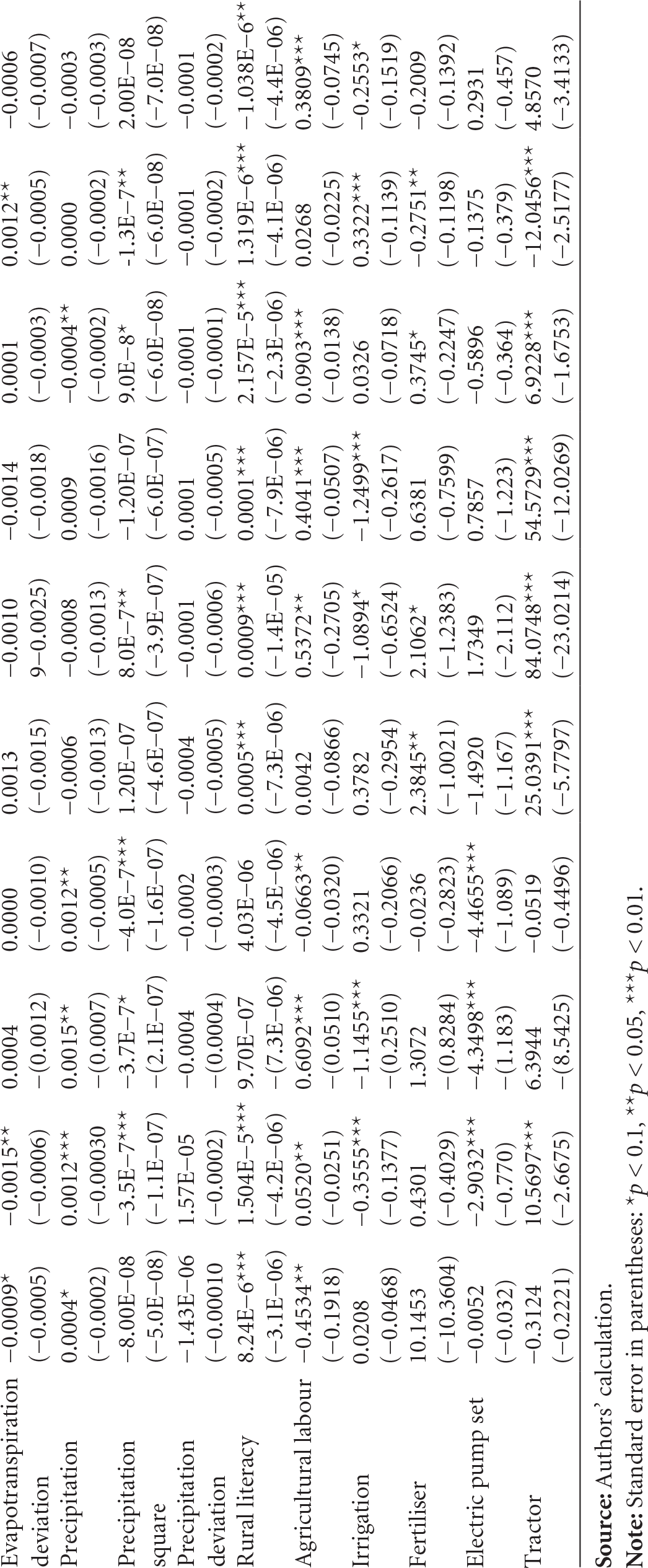
Variables	Oilseeds and Other Seeds								Cash Crops
Variables	Sesamum	Rapeseed and Mustard	Castor	Linseed	Sunflower	Safflower	Soyabean	Oilseeds	Sugarcane	Cotton
Average temperature	0.6192***	0.7804***	1.1476***	0.1201	0.1289	−1.7207***	0.2967	−0.0313	0.7467***	−0.6357***
Average temperature	(−0.1092)	(−0.1284)	(−0.2778)	(−0.1880)	(−0.4611)	(−0.5160)	(−0.2949)	(−0.0696)	(−0.1088)	(−0.1421)
Temperature square	−0.0114***	−0.0197***	−0.0182***	−0.0008	−0.0043	0.0327***	−0.0056	0.0013	−0.01469***	0.0164***
Temperature square	(−0.0027)	(−0.0032)	(−0.0068)	(−0.0047)	(−0.0102)	(−0.0127)	(−0.0072)	(−0.0017)	(−0.0027)	(−0.0036)
Temperature deviation	0.1274*	0.0108	−0.0809	0.0931	−0.2897	−0.5962*	−0.0935	−0.0182	0.0550	0.0726
Temperature deviation	(−0.0731)	(−0.0872)	(−0.1783)	(−0.1278)	(−0.2237)	(−0.3289)	(−0.2388)	(−0.0441)	(−0.0774)	(−0.0943)
Wind speed	−0.7964**	−1.2339***	−1.2690*	−1.0351*	−4.6779***	−0.6558	3.6612***	0.0731	0.3541	0.2432
Wind speed	(−0.3230)	(−0.3532)	(−0.6913)	(−0.6019)	(−1.1410)	(−1.3035)	(−1.3222)	(−0.1830)	(−0.3353)	(−0.3380)
Wind speed square	0.1531*	−0.0127	0.3595**	0.1020	1.3277***	0.5786	−1.0161***	−0.0187	−0.0193	−0.0727
Wind speed square	(−0.0814)	(−0.0936)	(−0.1768)	(−0.1682)	(−0.3177)	(−0.3555)	(−0.3571)	(−0.0480)	(−0.0855)	(−0.0893)
Wind speed deviation	0.0051	1.3084***	−0.4395	0.4786*	−0.0211	−1.7806***	0.3853	0.0859	−0.1272	0.3074*
Wind speed deviation	(−0.1487)	(−0.1671)	(*−0.3176)	(−0.2715)	(−0.4251)	(−0.6479)	(−0.4827)	(−0.0873)	(−0.1563)	(−0.1788)
Evapotranspiration	0.0012	−0.0088***	−0.0023	0.0011	0.0088**	−0.0332***	−0.0012	0.0017**	0.0057***	0.0014
Evapotranspiration	(−0.0010)	(−0.0016)	−(0.0029)	(−0.0024)	(−0.0043)	(−0.0105)	(−0.0053)	(−0.0008)	(−0.0011)	(−0.0013)
Evapotranspiration square	−4.80E−07	4.41E−6***	1.35E−06	−1.85E−06	−4.99E−5*	2.033E−5***	−6.00E−07	−9.4E−7*	−3.97E−7***	−1.52E−7*
Evapotranspiration square	(−6.5E−07)	(−1.0E−06)	−(1.9E−06)	(−1.6E−06)	(−2.7E−06)	(−6.3E−06)	(−3.4E−06)	(−5.4E−07)	(−7.1E−07)	(−8.0E−07)
Evapotranspiration deviation	−0.0009*	−0.0015**	0.0004	0.0000	0.0013	−0.0010	−0.0014	0.0001	0.0012**	−0.0006
Evapotranspiration deviation	(−0.0005)	(−0.0006)	−(0.0012)	(−0.0010)	(−0.0015)	9−0.0025)	(−0.0018)	(−0.0003)	(−0.0005)	(−0.0007)
Precipitation	0.0004*	0.0012***	0.0015**	0.0012**	−0.0006	−0.0008	0.0009	−0.0004**	0.0000	−0.0003
Precipitation	(−0.0002)	(−0.00030	−(0.0007)	(−0.0005)	(−0.0013)	(−0.0013)	(−0.0016)	(−0.0002)	(−0.0002)	(−0.0003)
Precipitation square	−8.00E−08	−3.5E−7***	−3.7E−7*	−4.0E−7***	1.20E−07	8.0E−7**	−1.20E−07	9.0E−8*	-1.3E−7**	2.00E−08
Precipitation square	(−5.0E−08)	(−1.1E−07)	−(2.1E−07)	(−1.6E−07)	(−4.6E−07)	(−3.9E−07)	(−6.0E−07)	(−6.0E−08)	(−6.0E−08)	(−7.0E−08)
Precipitation deviation	−1.43E−06	1.57E−05	−0.0004	−0.0002	−0.0004	−0.0001	0.0001	−0.0001	−0.0001	−0.0001
Precipitation deviation	(−0.00010	(−0.0002)	−(0.0004)	(−0.0003)	(−0.0005)	(−0.0006)	(−0.0005)	(−0.0001)	(−0.0002)	(−0.0002)
Rural literacy	8.24E−6***	1.504E−5***	9.70E−07	4.03E−06	0.0005***	0.0009***	0.0001***	2.157E−5***	1.319E−6***	−1.038E−6**
Rural literacy	(−3.1E−06)	(−4.2E−06)	−(7.3E−06)	(−4.5E−06)	(−7.3E−06)	(−1.4E−05)	(−7.9E−06)	(−2.3E−06)	(−4.1E−06)	(−4.4E−06)
Agricultural labour	−0.4534**	0.0520**	0.6092***	−0.0663**	0.0042	0.5372**	0.4041***	0.0903***	0.0268	0.3809***
Agricultural labour	(−0.1918)	(−0.0251)	−(0.0510)	(−0.0320)	(−0.0866)	(−0.2705)	(−0.0507)	(−0.0138)	(−0.0225)	(−0.0745)
Irrigation	0.0208	−0.3555***	−1.1455***	0.3321	0.3782	−1.0894*	−1.2499***	0.0326	0.3322***	−0.2553*
Irrigation	(−0.0468)	(−0.1377)	−(0.2510)	(−0.2066)	(−0.2954)	(−0.6524)	(−0.2617)	(−0.0718)	(−0.1139)	(−0.1519)
Fertiliser	10.1453	0.4301	1.3072	−0.0236	2.3845**	2.1062*	0.6381	0.3745*	−0.2751**	−0.2009
Fertiliser	(−10.3604)	(−0.4029)	−(0.8284)	(−0.2823)	(−1.0021)	(−1.2383)	(−0.7599)	(−0.2247)	(−0.1198)	(−0.1392)
Electric pump set	−0.0052	−2.9032***	−4.3498***	−4.4655***	−1.4920	1.7349	0.7857	−0.5896	−0.1375	0.2931
Electric pump set	(−0.032)	(−0.770)	−(1.183)	(−1.089)	(−1.167)	(−2.112)	(−1.223)	(−0.364)	(−0.379)	(−0.457)
Tractor	−0.3124	10.5697***	6.3944	−0.0519	25.0391***	84.0748***	54.5729***	6.9228***	−12.0456***	4.8570
Tractor	(−0.2221)	(−2.6675)	−(8.5425)	(−0.4496)	(−5.7797)	(−23.0214)	(−12.0269)	(−1.6753)	(−2.5177)	(−3.4133)

Source: Authors’ calculation.

Note: Standard error in parentheses: *p < 0.1, **p < 0.05, ***p < 0.01.

Notes

References

Anderson

, Bayer

P. E.

, & Edwards

(2020). Climate change and the need for agricultural adaptation. Current Opinion in Plant Biology, 56, 197–202. https://doi.org/10.1016/j.pbi.2019.12.006

Arora

N. K.

(2019). Impact of climate change on agriculture production and its sustainable solutions. Environmental Sustainability, 2(2), 95–96. https://doi.org/10.1007/s42398-019-00078-w

Aryal

J. P.

, Sapkota

T. B.

, Khurana

, Khatri-Chhetri

, Rahut

D. B.

, & Jat

M. L.

(2020). Climate change and agriculture in South Asia: Adaptation options in smallholder production systems. Environment, Development and Sustainability, 22(6), 5045–5075. https://doi.org/10.1007/s10668-019-00414-4

Ashkra, Khan

A. A.

, & Jadaun

K. K.

(2023). Estimating the potential effect of climate change on rice yield in India by considering the combined effects of temperature and rainfall. Bhartiya Krishi Anusandhan Patrika, 38(3), Article 3. https://doi.org/10.18805/BKAP649

Bera

(2021). Impact of climate change on pulse production and its mitigation strategies. Asian Journal of Advances in Agricultural Research, 14–28. https://doi.org/10.9734/ajaar/2021/v15i230147

Birthal

P. S.

, & Hazrana

(2019). Crop diversification and resilience of agriculture to climatic shocks: Evidence from India. Agricultural Systems, 173, 345–354. https://doi.org/10.1016/j.agsy.2019.03.005

Burke

, & Emerick

(2016). Adaptation to climate change: Evidence from US agriculture. American Economic Journal: Economic Policy, 8(3), Article 3. https://doi.org/10.1257/pol.20130025

Chandio

A. A.

, Jiang

, Rehman

, & Rauf

(2020). Short and long-run impacts of climate change on agriculture: An empirical evidence from China. International Journal of Climate Change Strategies and Management, 12(2), Article 2. https://doi.org/10.1108/IJCCSM-05-2019-0026

Chen

, & Gong

(2021). Response and adaptation of agriculture to climate change: Evidence from China. Journal of Development Economics, 148, 102557. https://doi.org/10.1016/j.jdeveco.2020.102557

10.

Choudhary

, Guha

, Kholova

, Pandravada

, Messina

C. D.

, Cooper

, & Vadez

(2020). Maize, sorghum, and pearl millet have highly contrasting species strategies to adapt to water stress and climate change-like conditions. Plant Science, Food Security under Climate Change, 295, 110297. https://doi.org/10.1016/j.plantsci.2019.110297

11.

CMIE. (2024). States of India. https://statesofindia.cmie.com/

12.

Cui

(2020). Climate change and adaptation in agriculture: Evidence from US cropping patterns. Journal of Environmental Economics and Management, 101, 102306. https://doi.org/10.1016/j.jeem.2020.102306

13.

Cui

, & Xie

(2022). Adapting agriculture to climate change through growing season adjustments: Evidence from corn in China. American Journal of Agricultural Economics, 104(1), Article 1. https://doi.org/10.1111/ajae.12227

14.

Da Cruz

T. V.

, & Machado

R. L.

(2023). Measuring climate change’s impact on different sugarcane varieties production in the South of Goiás. Scientific Reports, 13(1), 11637. https://doi.org/10.1038/s41598-023-36582-7

15.

Daloz

A. S.

, Rydsaa

J. H.

, Hodnebrog

Ø.

, Sillmann

, van Oort

, Mohr

C. W.

, Agrawal

, Emberson

, Stordal

, & Zhang

(2021). Direct and indirect impacts of climate change on wheat yield in the Indo-Gangetic plain in India. Journal of Agriculture and Food Research, 4, 100132. https://doi.org/10.1016/j.jafr.2021.100132

16.

, Xu

, Yi

, & McCarl

(2024). Climate change and winter wheat yields: The roles of freezing days and long-run adaptations. European Review of Agricultural Economics, 51(3), Article 3. https://doi.org/10.1093/erae/jbae015

17.

DeFries

, Liang

, Chhatre

, Davis

K. F.

, Ghosh

, Rao

N. D.

, & Singh

(2023). Climate resilience of dry season cereals in India. Scientific Reports, 13(1), Article 1. https://doi.org/10.1038/s41598-023-37109-w

18.

Di Falco

, & Chavas

J.-P.

(2006). Crop genetic diversity, farm productivity and the management of environmental risk in rainfed agriculture. European Review of Agricultural Economics, 33(3), 289–314. https://doi.org/10.1093/eurrag/jbl016

19.

Eliazer Nelson

A. R. L.

, Ravichandran

, & Antony

(2019). The impact of the Green Revolution on indigenous crops of India. Journal of Ethnic Foods, 6(1), 8. https://doi.org/10.1186/s42779-019-0011-9

20.

Famanta

, Randhawa

A. A.

, & Yajing

(2024). The impact of green FDI on environmental quality in less developed countries: A case study of load capacity factor based on PCSE and FGLS techniques. Heliyon, 10(7), e28217. https://doi.org/10.1016/j.heliyon.2024.e28217

21.

Farooq

M. A.

, Chattha

W. S.

, Shafique

M. S.

, Karamat

, Tabusam

, Zulfiqar

, & Shakeel

(2023). Transgenerational impact of climatic changes on cotton production. Frontiers in Plant Science, 14, 987514. https://doi.org/10.3389/fpls.2023.987514

22.

Gulati

, & Juneja

(2020). Farm mechanization in Indian agriculture with focus on tractors. SSRN Scholarly Paper No. 3689250. Social Science Research Network. https://doi.org/10.2139/ssrn.3689250

23.

Gull

, Bhat

T. A.

, Sheikh

T. A.

, Wani

O. A.

, Fayaz

, Nazir

, Saad

A. A.

, Jan

, Nazir

, & Rifat-un-Nisah. (2020). Climate change impact on pulse in India: A review. Journal of Pharmacognosy and Phytochemistry, 9(4), Article 4.

24.

Gupta

, Sen

, & Srinivasan

(2014). Impact of climate change on the Indian economy: Evidence from food grain yields. Climate Change Economics, 05(02), 1450001. https://doi.org/10.1142/S2010007814500018

25.

Harwood

(2021). Coming to terms with tropical ecology: Technology transfer during the early Green Revolution. International Journal of Agricultural Sustainability, 19(3–4), 305–318. https://www.tandfonline.com/doi/full/10.1080/14735903.2021.1908747

26.

Hussain

, Huang

, Ahmad

, Nanda

, Anwar

, Shakoor

, Zhu

, Cao

, Jin

, & Zhang

(2020). Rice production under climate change: Adaptations and mitigating strategies. In Fahad

, Hasanuzzaman

, Alam

, Ullah

, Saeed

, Khan

I. Ali

, & Adnan

(Eds), Environment, climate, plant and vegetation growth (pp. 659–686). Springer International Publishing. https://doi.org/10.1007/978-3-030-49732-3_26

27.

ICRISAT. (2024). District-level database. http://data.icrisat.org/dld/

28.

ICRISAT VDSA. (2024). VDSA home. https://vdsa.icrisat.org/

29.

IPCC. (2022). IPCC. https://archive.ipcc.ch/ipccreports/tar/wg2/index.php?idp=495

30.

Jans

, von Bloh

, Schaphoff

, & Müller

(2021). Global cotton production under climate change – implications for yield and water consumption. Hydrology and Earth System Sciences, 25(4), 2027–2044. https://doi.org/10.5194/hess-25-2027-2021

31.

Jaworski

C. C.

, Thomine

, Rusch

, Lavoir

A.-V.

, Wang

, & Desneux

(2023). Crop diversification to promote arthropod pest management: A review. Agriculture Communications, 1(1), 100004. https://doi.org/10.1016/j.agrcom.2023.100004

32.

Jyothsna

, Aakash, Reddy

P. M.

, & Setty

(2024). Impact of temperature variations on rice production. International Journal of Environment and Climate Change, 14(5), Article 5. https://doi.org/10.9734/ijecc/2024/v14i54166

33.

Kadiyala

M. D. M.

, Nedumaran

, Padmanabhan

, Gumma

M. K.

, Gummadi

, Srigiri

S. R.

, Robertson

, & Whitbread

(2021). Modeling the potential impacts of climate change and adaptation strategies on groundnut production in India. Science of The Total Environment, 776, 145996. https://doi.org/10.1016/j.scitotenv.2021.145996

34.

Karmacharya

, Jones

, Moufouma-Okia

, & New

(2017). Evaluation of the added value of a high-resolution regional climate model simulation of the South Asian summer monsoon climatology. International Journal of Climatology, 37(9), Article 9. https://doi.org/10.1002/joc.4944

35.

Katzenberger

, Schewe

, Pongratz

, & Levermann

(2021). Robust increase of Indian monsoon rainfall and its variability under future warming in CMIP6 models. Earth System Dynamics, 12(2), Article 2. https://doi.org/10.5194/esd-12-367-2021

36.

Kumar

, & Sharma

(2022). Impact of climate variation on agricultural productivity and food security in rural India. SSRN Scholarly Paper No. 4144089. Social Science Research Network. https://doi.org/10.2139/ssrn.4144089

37.

Lal

(2011). Implications of climate change in sustained agricultural productivity in South Asia. Regional Environmental Change, 11(1), 79–94. https://doi.org/10.1007/s10113-010-0166-9

38.

Lele

, & Goswami

(2017). The fourth industrial revolution, agricultural and rural innovation, and implications for public policy and investments: A case of India. Agricultural Economics, 48(S1), 87–100. https://doi.org/10.1111/agec.12388

39.

Maity

, Paul

, Lamichaney

, Sarkar

, Babbar

, Mandal

, Dutta

, Maity

P. P.

, & Chakrabarty

S. K.

(2023). Climate change impacts on seed production and quality: Current knowledge, implications, and mitigation strategies. Seed Science and Technology, 51(1), Article 1. https://doi.org/10.15258/sst.2023.51.1.07

40.

Meena

V. S.

, Verma

J. P.

, & Meena

S. K.

(2015). Towards the current scenario of nutrient use efficiency in crop species. Journal of Cleaner Production, 102, 556–557. https://doi.org/10.1016/j.jclepro.2015.04.030

41.

Mishra

, Sahu

N. C.

, & Sahoo

(2016). Impact of climate change on agricultural production of Odisha (India): A Ricardian analysis. Regional Environmental Change, 16(2), 575–584. https://doi.org/10.1007/s10113-015-0774-5

42.

Mishra

, Acharyya

, Chand

, Santos

C. A. G.

, Kar

, Das

P. P.

, Pattnaik

, da Silva

R. M.

, & Nascimento

T. V. M. do.

(2022). Analyzing shoreline dynamicity and the associated socioecological risk along the Southern Odisha Coast of India using remote sensing-based and statistical approaches. Geocarto International, 37(14), Article 14. https://doi.org/10.1080/10106049.2021.1882005

43.

Mohapatra

, Sharp

, Sahoo

A. K.

, & Sahoo

(2022). Decomposition of climate-induced productivity growth in Indian agriculture. Environmental Challenges, 7, 100494. https://doi.org/10.1016/j.envc.2022.100494

44.

Mohapatra

, Sharp

, & Sahoo

(2022). How changes in climate affect crop yields in eastern India. Climate Change Economics, 13(02), 2250001. https://doi.org/10.1142/S2010007822500014

45.

Nadkarni

M. V.

(2022). Crisis in Indian agriculture: Can it be overcome? Journal of Social and Economic Development, 24(1), Article 1. https://doi.org/10.1007/s40847-022-00202-3

46.

Neelima

A. S.

, & Kumar

K. N. R.

(2023). Impact of climate change on groundnut yield and its variability in Andhra Pradesh, India. Asian Journal of Agricultural Extension, Economics & Sociology, 41(2), Article 2. https://doi.org/10.9734/ajaees/2023/v41i21843

47.

Neupane

, Adhikari

, Bhattarai

, Rana

, Ahmed

, Sharma

, & Adhikari

(2022). Does climate change affect the yield of the top three cereals and food security in the world? Earth, 3(1), Article 1. https://doi.org/10.3390/earth3010004

48.

Okemo

, Wijesundra

, Nakandala

, Dillon

, Chandora

, Campbell

, Smith

, Hardner

, Cadorna

C. A.

, Martin

, Yahiaoui

, Garsmeur

, Pompidor

, D’Hont

, & Henry

R. J.

(2024). Crop domestication in the Asia Pacific region: A review. Agriculture Communications, 2(1), 100032. https://doi.org/10.1016/j.agrcom.2024.100032

49.

Ortiz-Bobea

, Ault

T. R.

, Carrillo

C. M.

, Chambers

R. G.

, & Lobell

D. B.

(2021). Anthropogenic climate change has slowed global agricultural productivity growth. Nature Climate Change, 11(4), 306–312. https://doi.org/10.1038/s41558-021-01000-1

50.

Padakandla

S. R.

(2016). Climate sensitivity of crop yields in the former state of Andhra Pradesh, India. Ecological Indicators, Navigating Urban Complexity: Advancing Understanding of Urban Social – Ecological Systems for Transformation and Resilience, 70, 431–438. https://doi.org/10.1016/j.ecolind.2016.06.008

51.

Patel

S. K.

, Sharma

, & Singh

G. S.

(2020). Traditional agricultural practices in India: An approach for environmental sustainability and food security. Energy, Ecology and Environment, 5(4), 253–271. https://doi.org/10.1007/s40974-020-00158-2

52.

Pillai

A. J.

, & Walia

(2024). Heat stress in Indian mustard (Brassica juncea L.): A critical review of impacts and adaptation strategies. Plant Cell Biotechnology and Molecular Biology, 25(5–6), Article 5–6. https://doi.org/10.56557/pcbmb/2024/v25i5-68673

53.

Ruane

A. C.

, & Rosenzweig

(2018). Climate change impacts on agriculture. Agriculture & Food Systems to 2050, 2, 161–191. https://doi.org/10.1142/9789813278356_0005

54.

Singh

A. K.

, Upadhyaya

, Kumari

, Sundaram

P. K.

, & Jeet

(2020). Role of agriculture in making India $5 trillion economy under corona pandemic circumstance: Role of agriculture in Indian economy. Journal of AgriSearch, 7(2), Article 2.

55.

Singh

, Sahany

, Singh

K. K.

, Robock

, & Xia

(2024). Future climate change impacts on rice in Uttar Pradesh, India’s most populous agrarian state. Earth’s Future, 12(5), Article 5. https://doi.org/10.1029/2023EF004009

56.

Singh

, & Singh

G. S.

(2017). Traditional agriculture: A climate-smart approach for sustainable food production. Energy, Ecology and Environment, 2(5), 296–316. https://doi.org/10.1007/s40974-017-0074-7

57.

Verma

, Gupta

, & Sen

(2020). Does climate change make foodgrain yields more unpredictable? Evidence from India. CESifo Working Paper No. 8161. https://doi.org/10.2139/ssrn.3555588

58.

Wang

, Vanga

S. K.

, Saxena

, Orsat

, & Raghavan

(2018). Effect of climate change on the yield of cereal crops: A review. Climate, 6(2), Article 2. https://doi.org/10.3390/cli6020041

59.

Wang

, Folberth

, Skalsky

, Wang

, Chen

, Liu

, Chen

, & Balkovic

(2022). Crop calendar optimization for climate change adaptation in rice-based multiple cropping systems of India and Bangladesh. Agricultural and Forest Meteorology, 315, 108830. https://doi.org/10.1016/j.agrformet.2022.108830

60.

World Bank. (2024). Employment in agriculture (% of total employment) (modeled ILO estimate)—India [Dataset]. https://data.worldbank.org/indicator/SL.AGR.EMPL.ZS?locations=IN

61.

Yadav

, Kumar

, Kim

S.-J.

, Srivastava

, Mohan

, & Ravichandran

(2024). Contrasting response of regional spring Arctic Sea ice variations on Indian summer monsoon rainfall. Remote Sensing of Environment, 311, 114247. https://doi.org/10.1016/j.rse.2024.114247