Impact of different models of agriculture on greenhouse gases (GHG) emissions: A sectoral approach

Abstract

It is estimated that farm practices are responsible for as much as 25–30% of greenhouse gas (GHG) emissions. The scale of such emissions from agriculture depends on the model to which that sector conforms. The aim of this study was to investigate how the attributes of particular models of agriculture (i.e. labour, capital, land productivity, machinery, chemical, energy and water inputs) affect GHG emissions at the sectoral level. We test the hypothesis that the productivity of capital and labour as well as the intensity of inputs affect GHG emissions differently in countries with varying levels of economic development. The results indicate that in the poorest countries, a significant barrier to sustainable development is mechanization. In moderately wealthy countries there is a lack of stimuli to implement energy-saving technologies, while in the richest countries it is desirable that mechanization and chemicalization be reduced in favour of energy-saving technologies.

Keywords

Agriculture greenhouse gases intensification sustainable development

Introduction

Scientists make efforts to conceptualize the term ‘sustainable development’ and to give sustainability a more practical and applicative dimension (Von Wirén-Lehr 2001; Van Cauwenbergh 2007). Definitions of sustainable development usually refer to the need to consider the economic, social and environmental aspects of development. This last element is taking on even greater importance in relation to agriculture, which is the chief component of the natural resources sector (NRS). Agriculture is a sector with particularly strong links to the natural environment, which also means that agriculture faces a broad range of challenges in the context of environmental well-being (Walls, 2006). The difficulty in assessing the impact of agriculture on the environment results primarily from the limited availability of data and the multiplicity of variables which might be used but also from the links between agriculture and other components of the NRS (e.g. some farms are also engaged in fishing or forestry). Environmental impact may be evaluated through the lens of greenhouse gas (GHG) emissions, maintenance of biodiversity or water and soil quality. Nonetheless, the most perceptible global effects currently arise from the first of these factors.

GHG emissions are among the most significant external effects of agricultural production having a global impact on the environment. It is estimated that farm practices are responsible for as much as 25–30% of GHGs, with particularly high emissions in the case of livestock production (Hamuda and Patko, 2010). Agriculture does not emit large quantities of carbon dioxide (CO₂), on average 15% of total GHG emission, since agricultural land stores up significant quantities of carbon, leading to a reduction in the presence of CO₂ in the atmosphere. The chief gases produced by agriculture are methane (CH₄) and nitrous oxide (N₂O). These gases have much greater potential to produce a greenhouse effect than CO₂. A single kilogram of methane has 25 times the global warming effect of a kilogram of CO₂, and a kilogram of nitrous oxide has 298 times the global warming effect of CO₂ (Eurostat, 2016; Lesschen et al., 2011). N₂O is emitted into the atmosphere from agricultural land chiefly as a result of microbiological processing of nitrogen fertilizers in the soil. Direct emissions of N₂O from the soil account for 25% and indirect emissions from the soil represent 16% of GHGs in European Union (EU) agriculture (EEA, 2009). Methane emissions are chiefly a result of the digestive processes of ruminants (mainly cattle and sheep). According to EEA (2009), CH₄ accounts for 59% of GHG emissions in EU livestock farming. The global proportions of N₂O and CH₄ in agriculture are similar (40/60).

The unclear relationships between farm practices and their impact on GHG emissions arise from the large number of indicators which might be used. These may be classified as effect based and means based (van der Werf and Petit, 2002). These efforts, however, are focused on the microeconomic level and most of the existing indicators are of that type. They show how farm practices (such as use of fertilizers, pesticides) at the farm level impact various aspects of the natural environment (Galan et al., 2007; Torrellas et al., 2013). The question is whether the microeconomic perspective is sufficient? Although there have been references to the need for a broader view on the NRS, including the agricultural sector (Payraudeau and van der Werf, 2005), as far as we are aware insufficient attempt has been made to explore the dependence of a sectoral model of agriculture in different parts of the world and the environmental impact produced by that sector. There are reports indicating macroeconomic determinants of GHG emissions, but these refer to the economy as a whole (EEA, 2016). According to the literature, the reduction in GHG emissions in the EU can be attributed to several factors (using the Kaya decomposition identity). Of these, the lower energy intensity of gross domestic product (GDP) plays the largest role, followed by the carbon intensity of energy, which reflects the lower use of very carbon-intensive fuels such as coal, and of fossil fuels in general. These two factors driving emissions down are partially offset by higher population and GDP per capita as well as by a higher share of non-energy-related (non-combustion) emissions, including agricultural production. Studies of this type relating specifically to the agriculture are nonetheless lacking.

The sectoral perspective is however of great importance for the shaping of agricultural policy towards small farms dominating the agricultural sector in many countries. If one considers a small farm as a holding that sells less than 50% of its agricultural output and consumes the remainder within the farm household, then there are over 6 million such units in the EU27 (FAO and OECD, 2012). Hence, the aim of this study was to investigate how sectoral characteristics (models) of agriculture affect GHG emissions across a sample of 40 countries over a long-term period. To obtain robust results, we divided the sample into clusters of countries where conditions for agricultural production at national level (i.e. level of support, GDP per capita, average farm size) were relatively similar.

Methodology

Our approach differs to a significant extent from those adopted in previous studies on the environmental impact of agriculture (Czyżewski and Kryszak, 2017). We evaluate environmental effects based on a scale of GHG emissions from the NRS (agriculture, hunting, forestry and fishing) in individual countries. We study the NRS as a whole and adopt an input–output approach based on a macroeconomic model of the economy, as pioneered by Leontief (1966). In the macroeconomic input–output table, the category ‘agriculture, hunting, forestry and fishing’ is viewed as a ‘proxy’ for agriculture. The source of the data is the World Input–Output Database¹ and the associated Socio Economic Accounts and Environmental Accounts (WIOD, 2016) as well as figures from Eurostat, Food and Agriculture Organization of the United Nations (FAOSTAT) and the World Bank (concerning number of farms, GDP and support for agriculture measured by the nominal rate of assistance (NRA) index). The study covers the period 1995–2009 in 40 countries. We divided our analysis into two stages. In the first, we attempt to address the effect of structural factors that constitute the conditions for agriculture development (Czyżewski and Kryszak, 2017):

GDP per capita (IMF, 2016);

Average size of a farm in a given country in hectares (source: Lowder et al., 2014);

Level of support to agriculture measured by the NRA in 2009 (from the World Bank’s Distortions to Agricultural Incentives database, Anderson, Nelgen 2013).

For this purpose, we performed cluster analysis (by Ward’s method) (Figure 1) using standardized values of the three listed structural variables. The disjointness of the clusters was verified using the Silhouette index S(i) as recommended by Gatnar and Walesiak (2004). The importance of the above-listed structural variables for GHG emissions has been confirmed by EEA (2016). We know that higher wealth of a country and its inhabitants is often correlated with higher per capita emissions (Aldy, 2006), while on the other hand it enables the implementation of modern, more environmental-friendly technologies. The introduction of consumption-based rather than production-based accounting of CO₂ emission changes to some extent popular beliefs about GHG emission. It turns out that countries such as China perform better, whereas Western Europe, the United States and Japan have even higher emissions (Davis and Caldeira, 2010). Aldy (2006) discusses an example of environmental Kuznets curve showing that firstly when per capita income grows the emission is also growing but when the level of income is sufficiently high, the emission may decrease. There is also uncertainty as to whether an increase in per capita income in itself leads to an increase in environmental awareness. Assistance in this regard may come from institutional stimuli, including agricultural and environmental policies, which stimulate pro-environmental methods of production. It is clear that richer countries have greater possibilities in this regard, but an increase in GDP per capita is not synonymous with a pro-environmental orientation of agricultural policy. There is also the issue of the agrarian structure, shaped both historically and geographically (i.e. depending on natural conditions), which we express by means of the average farm size.

Figure 1.

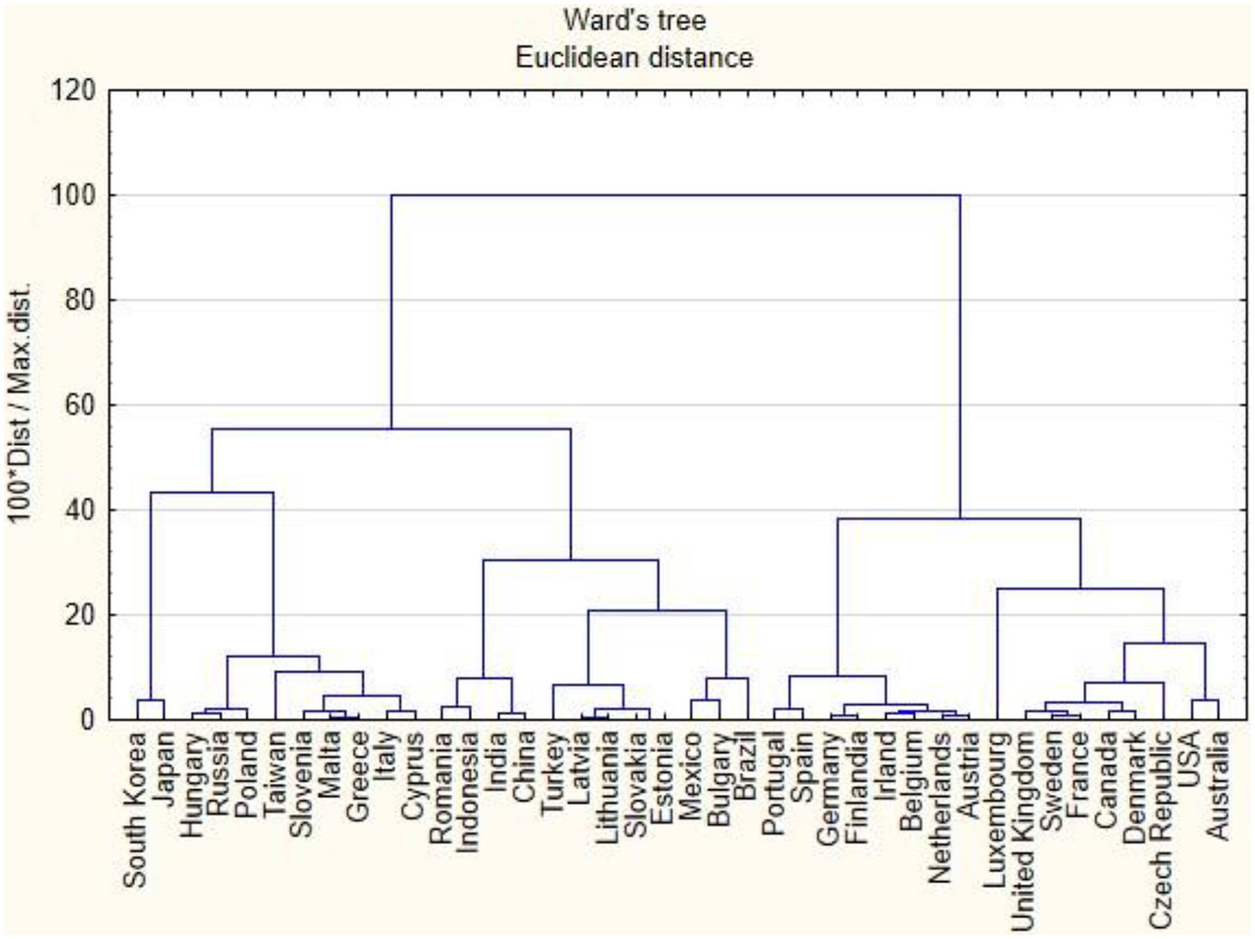
Clusters of countries according to the structural variables: GDP per capita, average size of farms and support to agriculture (NRA).

In the second stage, we computed panel regression models for each of the clusters A, B and C, beginning with the least wealthy countries, as in equation (1) (variables expressed in US dollars based on fixed prices from 1995):

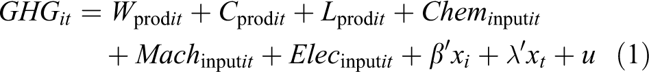
G H G_{i t} = W_{prod i t} + C_{prod i t} + L_{prod i t} + C h e m_{i nput i t} + M a c h_{input i t} + E l e c_{input i t} + β' x_{i} + λ' x_{t} + u

where,

i denotes a country; t denotes a year; GHG denotes total methane, nitrous oxide and carbon dioxide in tonnes of CO₂ equivalent per hectare; W _prod denotes labour productivity (own labour compensation, ‘000 US$ per 1 engaged); C _prod denotes capital productivity (‘000 US$ per Gross Fixed Capital Formation (GFCF) in ‘000 US$); L _prod denotes land productivity (agricultural output in ‘000 US$ per ha); Chem _input denotes chemical input (‘000 US$ per ha); Mach _input denotes machinery input (‘000 US$ per ha); Elec _input denotes electricity, gas and water supply (‘000 US$ per ha); Chem _input + Mach _input + Elec _input = ‘intensive input’; β′ is a vector of dummy variables for countries; λ′ is a vector of dummy variables for years; and u is a random error.

A linear form of the function was chosen, as this achieved the best fit. We believe that the above specification of variables reflects well the differentiation between agriculture models at sectoral level. The variables reflecting productivity (W _prod , C _prod , L _prod) enable the capture of a combination of labour intensity, capital intensity and land fertility. High labour intensity is a distinctive feature of subsistence agriculture and of the organic and conservation models (in the last case, however, in combination with higher capital profitability) (Aliber and Hart, 2009; FAO, 2016; OWF, 2016). High capital productivity is a feature of industrial agriculture and precision farming (Kansas State University, 2016, UCSUSA, 2016). Land productivity depends largely on natural factors (climate, soil quality). We treat intermediate consumption in the areas of mechanization, chemicalization, and consumption of energy and fuels as a ‘proxy’ for the diffusion of technological progress and knowledge in these areas. We assumed that the more modern a solution is used, the more likely it is environmental friendly. We selected these three groups of providers by means of production, because they make the greatest contributions to intermediate consumption in the agriculture (Eurostat use table). GHG emission stands for the dependent variable covering methane, nitrous oxide and carbon dioxide in kilogram CO₂ equivalent per hectare (Brander and Davis, 2012) produced by the NRS in a given country. To eliminate the effect of exchange rate fluctuations, all variables are expressed in ‘000 US dollars at 1995 prices. It is assumed that the differences in rates of inflation between countries are reflected in the dollar exchange rates of national currencies.

In the first step, the multicollinearity of the variables from model 1 was evaluated on the basis of variance inflation factors (VIFs). Variables not exceeding VIF = 5 were retained in the model (Chatterjee and Hadi, 2006). Next we computed ordinary least squares (OLS) base models. In case of rejection of the hypothesis of applicability of this approach (based on the Breusch–Pagan test), we computed panel models with fixed (FE) and random effects (RE). In these models, we introduced the variables step by step, checking whether the model was stable and whether the addition of a further variable caused changes in the signs of the other regression coefficients. The effect of the time factor was also shown in the panel models (as the linear trend variable), provided that it was significant in capturing the efforts of different countries to reduce GHG emissions.² The final models were computed taking into account the Beck–Katz robust standard errors (PCSE). In the results, we present, for each cluster, a final panel model with robust standard errors. We present the models in order from the poorest to the wealthiest countries.

Results and discussion

Three clusters of countries were identified (Figure 1 and Table 1). Cluster A includes 11 countries (Cyprus, Greece, Japan, South Korea, Malta, Poland, Russia, Slovenia, Taiwan, Hungary and Italy). Most of the countries in this cluster have moderate GDP values per capita purchasing power parity (PPP) (outside Japan and South Korea) (mean 21,774), while the average farm size is the lowest (5.24 ha), and the level of support (NRA) is high (mean 0.41). Cluster B consists of countries (Romania, Indonesia, India, China, Turkey, Latvia, Lithuania, Slovakia, Estonia, Mexico, Bulgaria, Brazil) that are usually relatively poor (mean GDP per capita 10,300), while the average level of support to agriculture is the lowest (mean NRA 0.18). In the countries of this cluster, the average farm size is usually small or moderate (mean, 14.4 ha). There are certain exceptions, however, such as Brazil, where large farms dominate, although its agricultural model is assigned as a whole to cluster B. The largest of the clusters is cluster C. This contains 17 relatively wealthy countries, with a mean GDP per capita (PPP) of 32,983 (Portugal, Spain, Germany, Finland, Ireland, Belgium, the Netherlands, Austria, Luxembourg, the United Kingdom, Sweden, France, Canada, Denmark, the Czech Republic, the United States and Australia). The mean value of support (NRA) is 0.26, and compared with the other clusters this value is relatively uniform between countries (low standard deviation). The average farm size for countries in this cluster is relatively high (see Table 1 for cluster characteristics). In each case, the FE model was found to be appropriate. All the models fit fairly well: the least square dummy variable (LSDV) R ² value ranges from 0.96 to 0.99, and within R ² from 0.17 to 0.51. Some variables were excluded due to excessive collinearity. All variables in the three models are statistically significant (p values do not exceed 0.1, except for one variable in cluster C for which p = 0.12).

Table 1.

Descriptive statistics of clusters A, B and C.

Statistic	A	B	C
Farm size in ha
Mean	5.24	14.40	274.59
Median	6.50	11.31	55.52
Standard deviation	3.73	14.47	771.69
Average GDP per capita (PPP)
Mean	21773.62	10299.51	32983.14
Median	22190.36	11235.53	31709.98
Standard deviation	5502.47	4195.11	10256.76
Average NRA
Mean	0.41	0.18	0.26
Median	0.31	0.18	0.28
Standard deviation	0.22	0.13	0.08

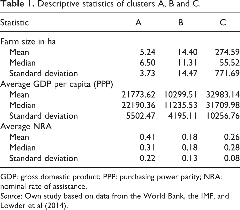
GDP: gross domestic product; PPP: purchasing power parity; NRA: nominal rate of assistance.

Source: Own study based on data from the World Bank, the IMF, and Lowder et al (2014).

Cluster B (Table 3) contained, relatively speaking, the poorest countries, with fragmented and highly polarized agriculture (farms of moderate size; Table 1), receiving limited state support. The appropriate model was found to be the panel model with FE. Due to strong collinearity, the variables ‘output per ha’ and ‘capital productivity’ were excluded. The model explains more than 96% of the variation in GHG emissions, taking account of individual country effects (LSDV R ² = 0.9657) which are constant in time (but vary in space). These are contained in the free term of the model but are expressed in detail by the dummy variables in the OLS model. The within R ² explains 17% of the intragroup (within) variation attributing variation in GHG emissions to the explanatory variables, which vary in time. Their variation in time seems to have significance. There is evidence for the lack of the pro-ecological evolution of the NRS model, in these countries. This is presented in Table 3, which shows that in 2002–2009 compared with 1995–2001, upward change in GHG emissions was visible.

Table 2.

Model for cluster A.^a

Variables	Coefficient	Standard error	Student’s t	p Value
Constant	306.104	42.894	71.363	<0.0001***
Capital compensation US$ per GFCF	489.875	128.181	38.218	0.0034***
Own labour comp. ‘000 US$ per farmer	86.104	143.272	60.098	0.0001***
Chemical input ‘000 US$ per ha	−1173.91	491.102	−2.3904	0.0379**
Electricity, gas, water supply ‘000 US$ per ha	7402.69	1665.76	44.440	0.0012***
Time (linear trend, unit = 1 year)	−150.639	216.035	−6.9729	<0.0001***
Descriptive statistics and tests
Type of statistics/test	GHG	Capital comp	Labour comp.	Chemical input	Electricity, gas, water
Mean	6289.480	−0.274	16.662	0.416	0.113
Standard deviation	4723.836	5.615	9.779	0.495	0.110
LSDV R ²	0.989712
Within R ²	0.333603

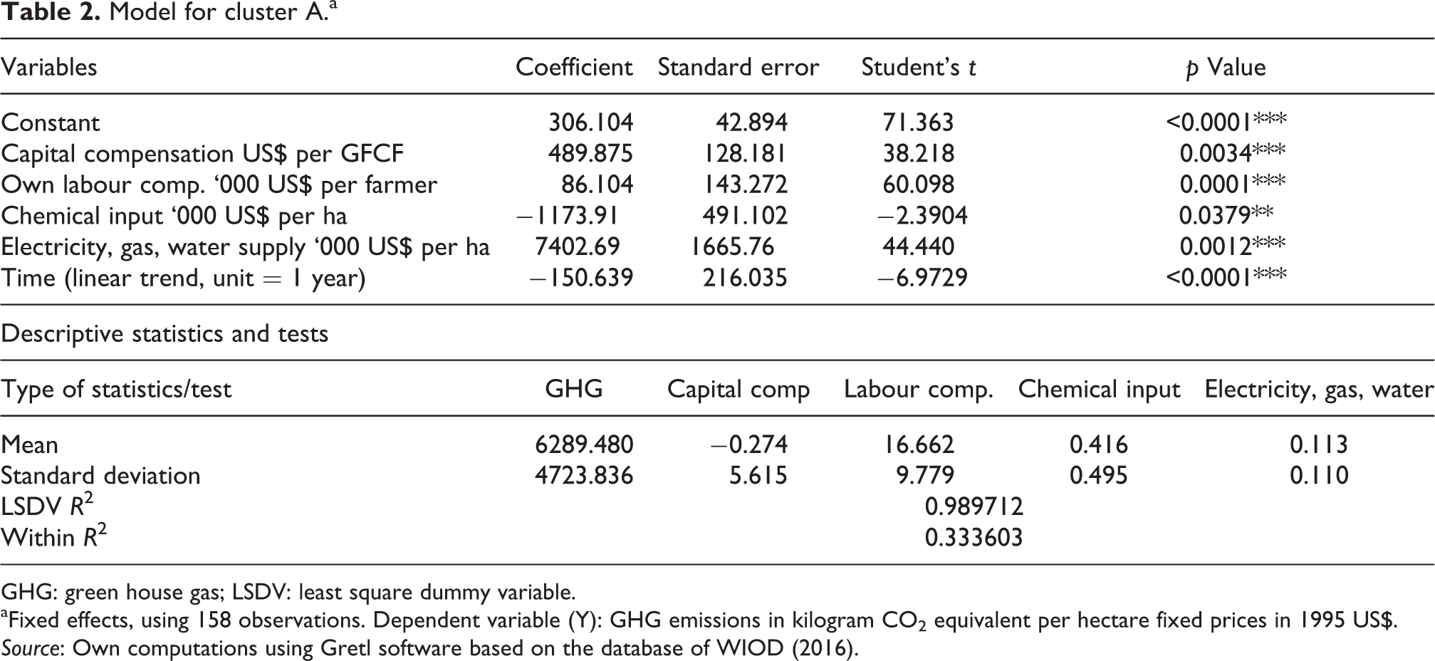
GHG: green house gas; LSDV: least square dummy variable.

^aFixed effects, using 158 observations. Dependent variable (Y): GHG emissions in kilogram CO₂ equivalent per hectare fixed prices in 1995 US$.

Source: Own computations using Gretl software based on the database of WIOD (2016).

Table 3.

Model for cluster B.^a

Variables	Coefficient	Standard error	Student’s t	p Value
Constant	1934.09	17.2906	111.8585	<0.0001***
Own labour comp. ‘000 US$ per engaged	363.743	0.932257	39.018	0.0025***
Chemical input ‘000 US$ per ha	−497.837	170.309	−2.9231	0.0139**
Machinery input ‘000 US$ per ha	1191.67	599.791	1.9868	0.0724*
Electricity, gas, water supply ‘000 US$ per ha	−1320.52	472.477	−2.7949	0.0174**
Time (2002–2009 compared with 1995–2001)	154.552	242.881	63.633	<0.0001***
Descriptive statistics and tests
Type of statistics/test	GHG	Labour comp.	Machinery input	Chemical input	Electricity, gas, water
Mean	1,967,337	19,291	0.044	0.198	0.056
Standard deviation	8,877,922	44,763	0.088	0.364	0.100
LSDV R ²	0.965738
Within R ²	0.170532

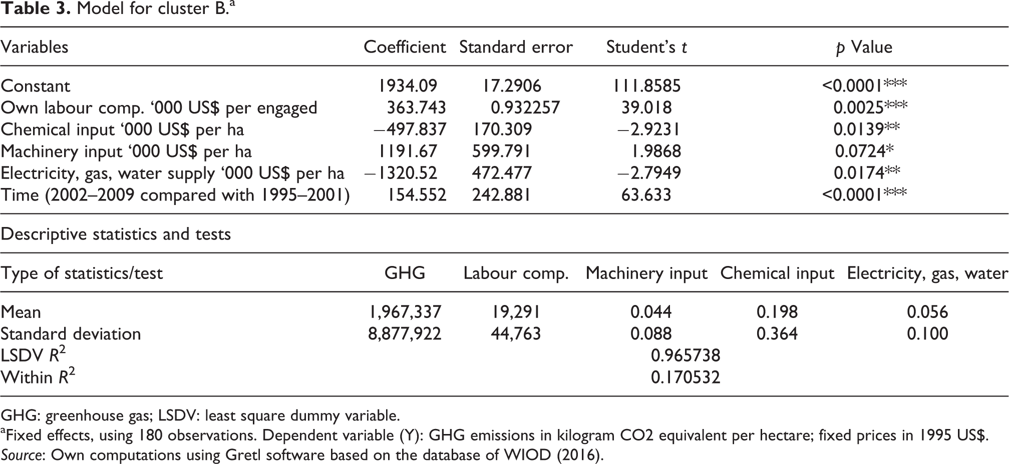
GHG: greenhouse gas; LSDV: least square dummy variable.

^aFixed effects, using 180 observations. Dependent variable (Y): GHG emissions in kilogram CO2 equivalent per hectare; fixed prices in 1995 US$.

Source: Own computations using Gretl software based on the database of WIOD (2016).

A surprising finding is that an increase in chemical inputs, in particular, leads to lower GHG emissions. Published data shows that technological progress in fertilizer production, and agro-technical progress relating to fertiliser use, is relatively speaking the fastest and leads to significant reduction in GHGs. The effectiveness of nitrogen application in highly developed countries has increased from 30% in the mid-1980s to an average of 60% at present (EEA, 2009). Many analyses have previously shown that when managed properly, fertilizer use fosters carbon capture. ‘When fertilizers are used properly, they help plants to produce more energy than is consumed during the production, transport and application of fertilizers. They also encourage the conversion of carbon dioxide to biomass through photosynthesis’ (IFA, 2009). The positive impact of agro-technology and fertilizer quality on emissions has been confirmed by many authors (Henault et al., 1998; Kaiser et al., 1998; Zieliński, 2014). Recent advances in fertilizer technology undoubtedly help to reduce N₂O emissions. ‘Timed-release fertilizers and fertilizers with nitrification inhibitors provide a gradual supply of nitrogen to the crop, synchronous with plant demand for nitrogen’ (Parton et al., 2011). We should also bear in mind that in cluster B the initial level of fertilizer use was low, and so it is undoubtedly subject to low-baseline effects. In spite of the increase in fertilizer use, the level of soil nitrogen concentration at which N₂O emissions increase was not attained. Conversely, in this cluster an increase in mechanization inputs leads to an increase in GHG emissions (by 1192 kg CO₂ equivalent per hectare for each US$1000). An increase in own labour compensation also produces higher emissions (in simplified terms, wealthy farmers do more harm to the environment). In highly simplified terms, then, we may adopt the interpretation that wealthier farmers (or fishermen) in these countries invest chiefly in machinery, but this involves investment in older devices which are less environmentally friendly.

Paradoxically, although these are the poorest countries in terms of GDP per capita, the mean unit compensation for own labour is higher than in cluster A (US$19,000 vs. US$16,000 per annum), although it is only half of the value for cluster C. Average use of chemicals per hectare is 50% lower than in cluster A but interestingly is 60% higher than in cluster C. This shows that progress in fertilizer usage is most visible in the wealthiest countries, probably because they use more effective fertilizers in smaller quantities per hectare. In view of the high standard deviations, however, it is necessary to treat the mean values of variables here with caution.

For the countries of cluster A (Table 2) (medium GDP per capita, small farms, fragmented agriculture, medium support), the FE model was again found to be appropriate. All variables in this model were statistically significant at α = 0.05. The model explains more than 98% of the variation in GHG emissions, taking account of the individual effects of countries (LSDV R ² = 0.9897), which are constant in time (but vary in space). The variables ‘output per ha’ and ‘machinery input’ were excluded due to collinearity (VIF > 5). The within-group R ² explains 33% of the variation within the cluster. This indicates that the evolution of the NRS model in these countries is faster than in cluster B. This is confirmed by analysis of the time influence (linear trend), given in Table 2, which shows that there is a clear downward trend in GHG emissions throughout the period (151 kg (CO₂ equivalent)) per hectare per year). Pro-environmental adaptations of the NRS were most visible in this group of countries, in the whole analysis period. An increase in chemical inputs leads to lower GHG emissions (by 1174 kg (CO₂ equivalent)) per hectare for every US$1000. The same interpretation as cluster B may be given, although in this case the diffusion of technological and agro-technical progress seems to be faster (the marginal effect is stronger). One of the reasons is probably the higher level of support given to agriculture.

At the same time, increases in labour compensation and in return on capital lead to higher GHG emissions, which is in line with environmental Kuznets curve theory (Aldy, 2006). We may therefore adopt the assumption, in simplified terms, that wealthier farmers in these countries are investing not in modern fertilizers but in energy-intensive technologies that are less friendly to the environment (probably technologies relating to livestock production, which generates more GHG than crop production and substitutes manure and slurry for mineral fertilizer) (Gołębiewska, 2010). For example, in a research conducted in Poland, the authors showed that in the beginning of the period (1996–2000) Polish farmers invested mainly in machinery and other technical devices. However, in the future they are likely to invest in buildings and their improvement. Both these investments are connected with high energy use.

The variable ‘electricity, gas, water supply’ has a negative effect on GHG emissions in this group. This may be an effect of the large share of livestock production in a whole agricultural sector. In 1995, the value of livestock production in total agricultural production in this cluster (excluding Taiwan) was 37%. In 2009, it increased to 39% (own calculations based on FAOSTAT data). Interestingly, the average return on capital in this group was negative, which supports the hypothesis of investment in obsolescent technologies. The intensity of chemical application is the highest (US$400 vs. US$130/ha/annum in the cluster containing the wealthiest countries). The high standard deviations again indicate the need for caution when considering the mean values of the variables.

In the cluster C countries (Table 4) (high GDP per capita, large farms, homogeneous agriculture, high support), the FE model again proved appropriate. It is noteworthy that in this model the variables ‘own labour compensation’ and ‘energy consumption’ take negative signs. This indicates that it is possible to combine environmental and socioeconomic goals (a win-win situation). Similar conclusions were reached by German et al (2017). Cluster C is dominated by the wealthy countries of the EU. It may be said that the European Agricultural Model, in spite of criticism and claims that its pro-environmental measures are merely ‘for show’ (Erjavec and Erjavec, 2015), has the greatest chance of realizing the concept of sustainable development. Our model explains 99% of the variation in GHG emissions, taking account of the individual effects of countries (LSDV R ² = 0.9956), which are constant in time (but vary in space). The variables ‘output per ha’ and ‘capital productivity’ were excluded due to collinearity. The within-group R ² explains 50% of the variation within the cluster. This indicates rapid implementation of technical progress and evolution of the NRS model compared with the other clusters. Nonetheless, the time factor was found to be statistically less significant (p = 0.15) with the lower pro-ecological effect compared to cluster A.

Only in this model does an increase in own labour compensation lead to lower GHG emissions, that is to say, wealthier farmers do less harm to the environment. In simplified terms, we may thus adopt the interpretation that wealthier farmers (or fishermen) in these countries invest in energy-saving, environmental-friendly technologies (OECD, 2001), which is the evidence of the increasing environmental awareness and agro-technical knowledge as well as rapid diffusion of technical progress in that area.

The marginal effect of the variable ‘electricity, gas, water supply’ is exceptionally strong: an increase in spending by US$1000 leads to a decrease in GHG emissions by 2784 kg (CO₂ equivalent per hectare). This is the evidence of rapid progress in the field of energy-saving technologies. This view is shared by other authors who point out that a key element in pro-environmental farm practices that reduce GHG emissions is effective irrigation (IFA, 2009). The variables representing machinery and chemical inputs do nonetheless have positive signs, which mean that in this group of countries opportunities for further pro-environmental progress in reducing CO₂ emissions in these areas are limited. This result has also been corroborated by other studies (Thirtle et al., 2004). As regards the descriptive statistics, own labour compensation was the highest in this group, while the value of chemical inputs was relatively speaking the lowest.

Table 5 summarizes the direction and relative strength of the influence of particular variables (ceteris paribus) on GHG emissions (an upward-pointing arrow indicates a positive effect). The downward arrows in the ‘intensive input’ (grey shading) indicate problematic areas in agriculture development. An interesting evolutionary path can be observed in this area by analysing in turn the poorest, the moderately wealthy and then the wealthiest countries: Initially it is mechanization that is most problematic for the environment, then consumption of energy (electricity, gas and water), while at a higher level of development the most problematic factors are chemicalization as well as mechanization.

Table 4.

Model for cluster C^a.

Variables	Coefficient	Standard error	Student’s t	p Value
Constant	4746.82	216.224	219.533	<0.0001***
Own labour comp. ‘000 US$ per farmer	−28.3119	837.767	−3.3795	0.0038***
Chemical input ‘000 US$ per ha	2025.85	1241.68	16.315	0.1223
Machinery input ‘000 US$ per ha	5390.72	1174.78	45.887	0.0003***
Electricity, gas, water supply ‘000 US$ per ha	−2784.39	1152.88	−2.4151	0.0281**
Time (linear trend, unit = 1 year)	−7.75912	519.346	−1.4940	0.1546
Descriptive statistics and tests
Type of statistics/test	GHG	Labour comp.	Chemical input	Machinery input	Electricity, gas, water
Mean	4,152,974	28,697	0.126	0.051	0.091
Standard deviation	3,961,515	14,422	0.116	0.068	0.196
LSDV R ²	0.995662
Within R ²	0.502889

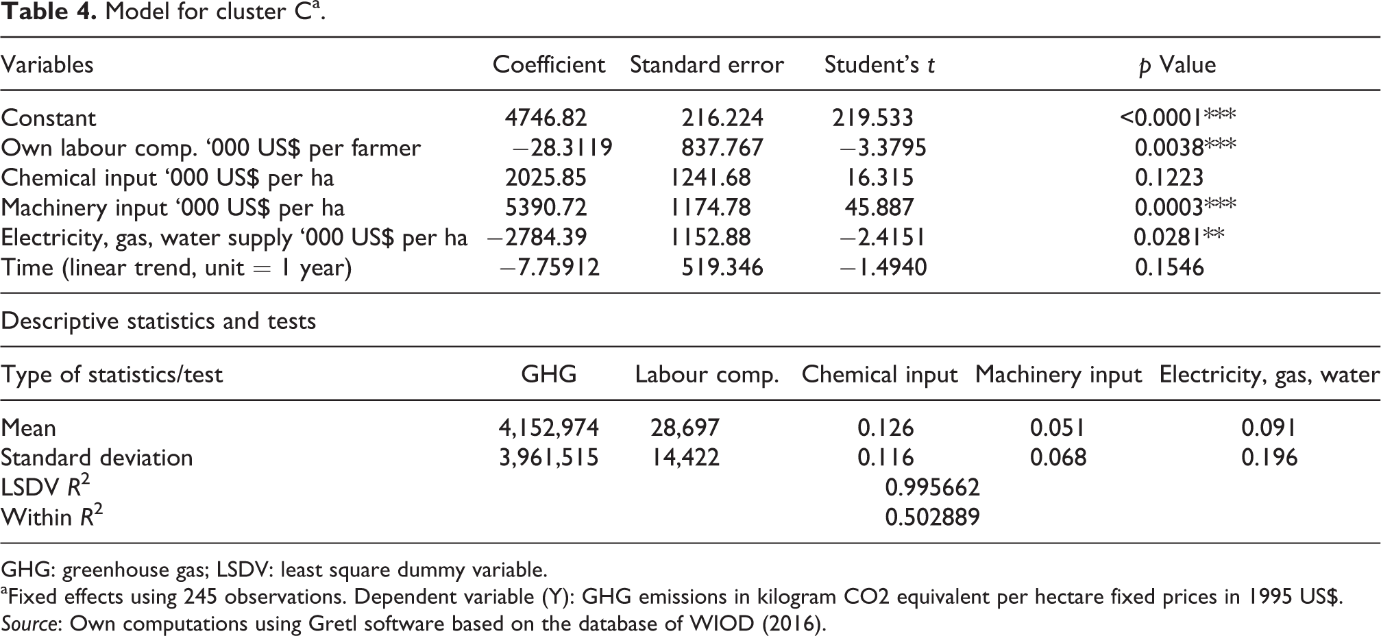
GHG: greenhouse gas; LSDV: least square dummy variable.

^aFixed effects using 245 observations. Dependent variable (Y): GHG emissions in kilogram CO2 equivalent per hectare fixed prices in 1995 US$.

Source: Own computations using Gretl software based on the database of WIOD (2016).

Table 5.

Comparison of marginal effects for models A, B and C.

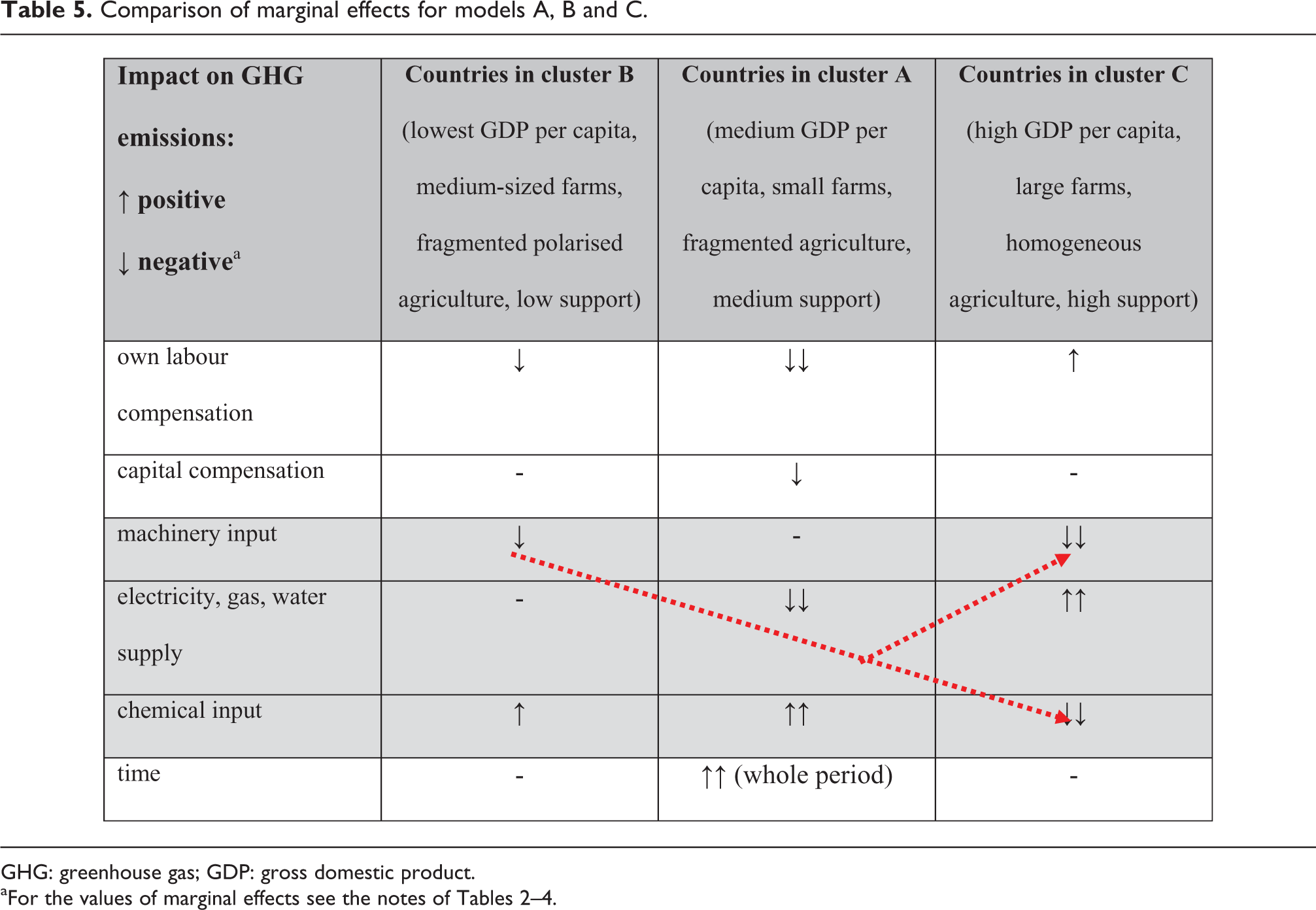
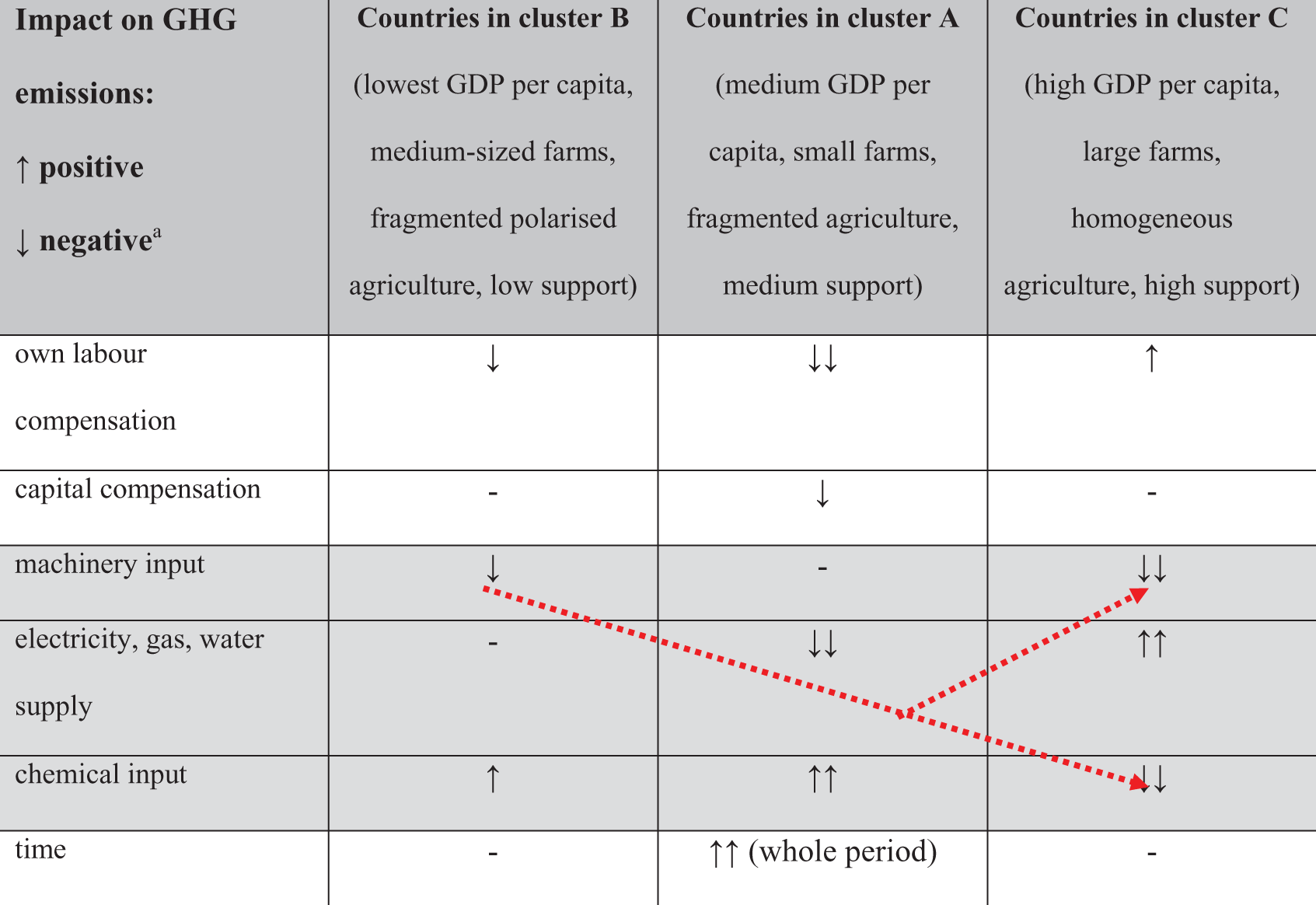
GHG: greenhouse gas; GDP: gross domestic product.

^aFor the values of marginal effects see the notes of Tables 2 –4.

Concluding comments

This analysis provides evidence that the conflict between the attainment of environmental and socioeconomic goals in the NRS is one that can be reduced. An example is provided by cluster C, which consists largely of countries of the ‘old’ EU15. Our models indicate a positive correlation in these countries between the level of labour compensation and the attainment of environmental goals in the form of reduced GHG emissions. This provides a partial response to the doubts expressed in the cited report (OECD, 2001). Higher wealth of farmers (fishermen, foresters), evaluated in terms of their income, favours the attainment of environmental goals on condition that they make use of energy-saving technologies. Further research will attempt to determine to what degree this is caused by increased awareness among farmers and by the requirements of agricultural and environmental policy or simply by the possibility of investing in more environmental-friendly technologies.

A second general finding is the indication of problem areas in the pro-ecological development of the NRS in the analysed clusters, which ought in principle to be the focus of agricultural and environmental policy. The aim is to indicate a general direction for action and not to lay down detailed guidelines. Among the poorest countries, a significant barrier to the sustainable development of the NRS is mechanization. In the moderately wealthy countries, there is a lack of market conditions and stimuli for the implementation of energy-saving technologies – such conditions ought therefore to be created. In the wealthiest countries, it is desirable that mechanization and chemicalization be limited in favour of energy-saving technologies.

European agriculture made the greatest progress in reducing quantities of GHG emitted per kilocalorie of agricultural production. In 1991–2009, pollution from agricultural production in Europe per capita fell by 22%, and in spite of the high density of population, this is relatively low on a global scale. This results from changes made to agriculture in the EU and may be linked both to the implementation of pro-environmental policy in agriculture, particularly since the early 1990s when the MacSharry reform realigned the principles of the Common Agricultural Policy, and to technological progress expressed by energy-saving technologies and renewable energy sources (Poczta and Baer-Nawrocka, 2016). However, our models show that in the countries of clusters B and A, the market conditions do not encourage the investment of capital in such solutions of environmental-friendly technologies . Thus, it shall be recalled that support for income will not suffice to achieve sustainable development.

Footnotes

Declaration of conflicting interests

The author(s) declared no potential conflicts of interest with respect to the research, authorship, and/or publication of this article.

Funding

The author(s) received no financial support for the research, authorship, and/or publication of this article.

Notes

References

Aldy

(2006) Per capita carbon dioxide emissions: convergence or divergence?. Environmental and Resource Economics 33(4):533–555.

Aliber

Hart

(2009) Should subsistence agriculture be supported as a strategy to address rural food insecurity? Agrekon 48(4):434–458.

Anderson

Nelgen

(2013) Updated national and global estimates of distortions to agricultural incentives, 1955 to 2011. Available at: www.worldbank.org/agdistortions (accessed 30 September 2016).

Brander

Davis

(2012) Greenhouse Gases, CO2, CO2e, and Carbon: What Do All These Terms Mean? Ecometrica. Available at: http://ecometrica.com/assets//GHGs-CO2-CO2e-and-Carbon-What-Do-These-Mean-v2 (30 September 2016).

Chatterjee

Hadi

(2006) Regression Analysis by Example. Hoboken, NJ: Wiley-Interscience.

Czyżewski

Kryszak

(2017) Wpływ typów rolnictwa na emisję gazów cieplarnianych. Wieś i Rolnictwo 1(174): 99–122.

Davis

Caldeira

(2010) Consumption-based accounting of CO2 emissions. Proceedings of the National Academy of Sciences 107(12):5687–5692.

EEA (2009) Technical Report 4/2009. Available at: http://www.copa-cogeca.be/Download.ashx?ID=836589 (accessed 30 September 2016).

EEA (2016) European Environment Agency, Analysis of key trends and drivers in greenhouse gas emissions in the EU between 1990 and 2014. Available at: http://www.eea.europa.eu/publications/analysis-of-key-trends-ghg/download (accessed 30 September 2016).

10.

Erjavec

(2015) Greening the CAP’ – Just a fashionable justification? A discourse analysis of the 2014–2020 CAP reform documents. Food Policy 51:53–62. DOI: 10.1016/j.foodpol.2014.12.006.

11.

Eurostat (2016) Greenhouse gas emissions by industries and households. Available at: http://ec.europa.eu/eurostat/statisticexplained/index.php/Greenhouse_gas_emissions_by_industries_and_households#CO2.C2.A0equivalents (accessed 30 September 2016).

12.

FAO (2016) Agriculture and consumer protection department, conservation agriculture. What is conservation agriculture? Available at: http://www.fao.org/ag/ca/1a.html (accessed 30 September 2016).

13.

FAO and OECD (2012) Sustainable agricultural productivity growth and bridging the gap for small family farms. Interagency Report to the Mexican G20 Presidency. Available at: https://cgspace.cgiar.org/bitstream/handle/10947/2702/Sustainable_Agricultural_Productivity_Growth_and_Bridging_the_Gap_for_Small-Family_Farms.pdf?sequence=1 (accessed 30 September 3016).

14.

Galan

Peschard

Boizard

(2007) ISO 14 001 at the farm level: analysis of five methods for evaluating the environmental impact of agricultural practices. Journal of Environmental Management 82(3):341–352.

15.

Gatnar

Walesiak

(eds.) (2004) Metody Statystyczne Analizy Wielowymiarowej w Badaniach Marketingowych. Wrocław: Wydawnictwo Akademii Ekonomicznej im. O. Langego.

16.

Genty

Arto

Neuwahl

(2012) Final database of environmental satellite accounts: technical report on their compilation. WIOD Documentation. Available at: http://www.wiod.org/publications/source_docs/Environmental_Sources.pdf (accesed August 2016).

17.

German

Thompson

Benton

(2017) Relationships among multiple aspects of agriculture’s environmental impact and productivity: a meta-analysis to guide sustainable agriculture. Biological Reviews 92(2): 716–738.

18.

Golebiewska

(2010) The directions of investment in the farms depend on the strength of their markets relations. Roczniki Nauk Rolniczych Seria G 97(4):60–68.

19.

Gouma

Timmer

De Vries

(2014) Employment and compensation in the WIOD Socio-Economic Accounts (SEA): revision for 2008–2009 and new data for 2010/2011. World Input-Output Database. Available at: http://www.wiod.org/protected3/data13/update_sep12/SEA%20Sources_June2014.pdf (accessed 30 September 2016).

20.

Hamuda

HEAFB

Patkó

(2010) Relationship between environmental impacts and modern agriculture. Óbuda University e-Bulletin 1:87–98.

21.

Henault

Devis

Page

. (1998) Nitrous oxide emissions from different soil and land management conditions. Biology Fertilizations Soils 26:199–207.

22.

IFA (2009) International Fertilizer Industry Association, Fertilizers, Climate Change and Enhancing Agricultural Productivity Sustainably, Paris, July, pp. 3–10. Available at: https://pl.scribd.com/document/61275156/2009-Ifa-Climate-Change (accessed 30 September 2016).

23.

IMF (2016) World Economic Outlook Database. April 2016 edition. Available at: http://www.imf.org/external/pubs/ft/weo/2016/01/weodata/index.aspx (accessed 30 September 2016).

24.

Kaiser

Kohrs

Kucke

. (1998) Nitrous oxide release from arable soil: importance of N-fertilisation, crops and temporal variation. Soil, Biology Biochemistry 30:1553–1563.

25.

Kansas State University—Biological and Agricultural Engineering Department (2016) Precision Agriculture: Tomorrow’s future here today. Available at: http://www.bae.ksu.edu/precisionag/ (accessed 30 September 2016).

26.

Leontifef

(1966) Input-Output Economics. New York: Oxford University Press.

27.

Lesschen

Velthof

G L

de Vries

. (2011) Differentiation of nitrous oxide emission factors for agricultural soils. Environmental Pollution 159:3215–3222.

28.

Lowder

Skoe

Singh

(2014) What do we really know about the number and distribution of farms and family farms in the world? Background paper for the State of Food and Agriculture 8. ESA Working Paper No. 14–02. Rome, FAO.

29.

OECD (2001) Environmental Indicators for Agriculture: Methods and Results. Paris: Organisation for Economic Co-operation and Development. Available at: http://www.oecd.org/tad/sustainable-agriculture/1916629.pdf (accessed 30 September 2016).

30.

Organic World Foundation (2016) Making a difference, inspiring action – that is what organic agriculture is. Available at: http://www.organicworldfoundation.org/organic_agriculture.html (accessed 30 September 2016).

31.

Parton

Del Grosso

Marx

. (2011) Agriculture’s role in cutting greenhouse gas emissions. Issues in Science and Technology 27(4):29–32.

32.

Payraudeau

van der Werf

H M

(2005) Environmental impact assessment for a farming region: a review of methods. Agriculture, Ecosystems & Environment 107(1):1–19.

33.

Poczta

Baer-Nawrocka

(2016) The sustainability of agriculture in the European Union against a global backdrop. In: Czyżewski

(ed) Political rents of european farmers in the sustainable development paradigm. International, national and regional perspective. Warsaw: Polish Scientific Publishers PWN, pp. 60–68.

34.

Thirtle

Lin

Holding

. (2004) Explaining the decline in UK agricultural productivity growth. Journal of Agricultural Economics 55(2):343–366.

35.

Timmer

Dietzenbacher

Los

. (2015) An illustrated user guide to the world input–output database: the case of global automotive production. Review of International Economics 23(3):575–605.

36.

Torrellas

Assumpció

Montero

(2013) An environmental impact calculator for greenhouse production systems. Journal of Environmental Management 118:186–195.

37.

UCSUSA (2016) Union of concerned scientists, industrial agriculture: the outdated, unsustainable system that dominates U.S. food production. Available at: http://www.ucsusa.org/our-work/food-agriculture/our-failing-food-system/industrial-agriculture (accessed 30 September 2016).

38.

Van Cauwenbergh

Biala

Bielders

. (2007) SAFE—A hierarchical framework for assessing the sustainability of agricultural systems. Agriculture, Ecosystems & Environment 120(2):229–242.

39.

van der Werf

Petit

(2002) Evaluation of the environmental impact of agriculture at the farm level: a comparison and analysis of 12 indicator-based methods. Agriculture Ecosystems & Environment 93(1):131–145.

40.

Von Wirén-Lehr

(2001) Sustainability in agriculture—an evaluation of principal goal-oriented concepts to close the gap between theory and practice. Agriculture, Ecosystems & Environment 84(2):115–129.

41.

Walls

(2006) Agriculture and Environment, SCAR Foresight Group, European Comission.

42.

WIOD (2016) World input-output database. Available at: http://www.wiod.org/new_site/home.htm (accessed 20 September 2016).

43.

Zieliński

(2014) Emission of greenhouse gases and effectiveness of functioning of Polish farms with field crops. Problemy Rolnictwa Światowego 14(XXIX), no 3: 226–236.