Cabinets,Prime Ministers,and Corruption: A Comparative Analysis of Parliamentary Governments in Post-War Europe

Abstract

Why are some states more corrupt than others? Drawing on the literature on governance in parliamentary democracies, we suggest that the degree of corruption depends on the ability of key political actors to control ministers who have been delegated power. We argue that the Prime Minister has incentives to limit corruption within the cabinet and has the ability to do so when there are certain “control mechanisms” at hand. One such mechanism is the PM’s ability to fire or demote ministers who are not behaving in accordance with his or her wishes. We hypothesize that governmental corruption will be lower in systems where the constitution grants the PM strong powers. Using a new dataset (Varieties of Democracy), which provides more specific measures on high-level corruption across a longer time period, we analyze corruption in 26 West and East European democracies over the post-war period and find support for our hypothesis.

Keywords

coalition governments government corruption Prime Ministers principal–agent theory parliamentary systems

Introduction

Why are some governments more corrupt than others? Why do high-level officials in some countries seem to “extract more rents” than others? There is a large literature focusing on explaining the existence of such abuse across countries and over time, where some scholars have focused on the role of various political–institutional features within democratic systems, for example, investigating the impact of characteristics that can be seen as “accountability enhancing” (see, for example, Schwindt-Bayer and Tavits, 2016). Our aim here is to contribute to the literature on institutional features that constrain corruption.

We present a complementary argument about what political–institutional features should influence corruption, taking our starting point in the so-called “parliamentary chain of delegation,” which suggests that power relationships in parliamentary democracies can be described as a chain with a number of links. In this chain, voters are the ultimate principals who delegate power to legislators through elections. However, voters only indirectly delegate power to cabinet members in a parliamentary system, and we here focus on the fact that the Prime Minister (PM) as a principal directly delegates power to line ministers within the cabinet and also has the power to hold them accountable (see, for example, Strøm, 2003).

We frame corruption as a principal–agent problem (e.g. Rose-Ackerman, 1978), focusing on the delegation relationship between the PM and his or her cabinet ministers. Our main expectation is that corruption among high-level officials should be lower in systems where the constitutional power of the PM is high and where the PM has the ability to control corruption in cabinet. Our theoretical argument is based on an assumption that the PM has stronger incentives than individual ministers to limit corruption within the cabinet, since policy outcomes are less likely to be in line with his or her preferences when ministers are corrupt. Following the previous literature on coalition governance, the PM should prefer to limit “ministerial drift,” whereas individual ministers have incentives and the opportunity to “drift” from the overall government policy in their departments, unless there are some control mechanisms in place. One such control mechanism is the PM’s ability to fire or demote those ministers who are not behaving in accordance with the PM’s wishes (see, for example, Bergman et al., 2003). The PM’s constitutional powers is an institutional feature that has not been in focus in the previous corruption literature, and we, thus, make a theoretical contribution by introducing this argument.

We make an empirical contribution to the literature by evaluating our hypotheses using a completely new dataset on corruption, drawing on the Varieties of Democracy data (Coppedge et al., 2015), allowing us to obtain more specific measures on the perception of corruption across longer periods of time (McMann et al., 2016). We evaluate our hypotheses by adding data on Western and Eastern European cabinets during the post-war period from the European Representative Democracy Data Archive (Andersson et al., 2014). Although not conclusive, since both corruption and PM powers are slow-moving characteristics, our results indicate that corruption is significantly lower when the PM has strong constitutional powers, suggesting that a strong PM is able to reduce agency problems within the cabinet.

Theory and Hypotheses

Previous Research on Political Institutions and Corruption

As described by Daniel Treisman (2007: 211), “Corruption is usually understood to mean the ‘misuse of public office for private gain,’ where the ‘private gain’ may accrue either to the individual official or to groups or parties to which he belongs.” Leslie Schwindt-Bayer and Margit Tavits (2016: 5) describe two types of corruption, “street-level petty corruption” and “systemic grand corruption,” where the latter is in focus in their study of clarity of responsibility. Grand corruption refers to the “extraction of rents and collection of kick-backs for major public projects by high-level officials” (see also Rose-Ackerman, 1999).

There is a large literature focusing on explaining the existence of such abuse across countries and over time, where some scholars have focused on the level of economic development (e.g. La Porta et al., 1999), whereas others have focused on the role of democratic institutions (e.g. Bäck and Hadenius, 2008). However, even within democratic systems, there is variation in corruption levels, and thus, scholars have looked at other political–institutional features as predictors of perceived corruption (see Treisman, 2007).

Drawing on such work on political institutions, Margit Tavits (2007: 218) presents an argument about clarity of responsibility, arguing that some political–institutional features can be seen as “accountability enhancing.” The main argument is that “political corruption depends on the effectiveness of the democratic process, i.e. the ability of the voters to monitor their representatives, to detect those responsible for unsatisfactory outcomes, and to hold them accountable by voting them out of office.” Tavits evaluates this argument by looking at a number of indicators, drawing on the work by Bingham Powell (2000). She shows, in a comparative analysis, that cabinets with higher duration, and legislatures with fewer parties, tend to be associated with lower corruption. In a more recent study, Schwindt-Bayer and Tavits (2016) find additional support for the clarity of responsibility argument using cross-sectional data, individual-level survey data, and experimental data. We here develop a theoretical claim that is complementary to the clarity of responsibility argument, drawing on the literature on how parties govern in parliamentary democracies.

The Literature on Governance in Multiparty Cabinets

The literature on coalition governance takes its starting point in the “parliamentary chain of delegation,” which describes power relationships in a parliamentary democracy as a chain with four links, where (1) citizens delegate power to representatives, (2) who delegate power to a cabinet and a PM, (3) who delegates power to line ministers within the cabinet, and (4) ministers, as heads of department, in turn, delegate to civil servants (e.g. Strøm, 2003).

Several scholars have applied principal–agent theory to analyze delegation problems within parliamentary systems, and two main threats to the principal’s ability to control the agent have been identified. The problem of adverse selection arises when the principal does not have access to relevant information about potential agents before selection. Moral hazard problems arise when agents, once selected, have motives and opportunity to act in ways that are contrary to the principal’s interests. What is, thus, important to note is that in each step of the chain where power is delegated from a principal to an agent, there also has to be a way for the principal to hold the agents accountable. Put differently, there has to be some “control mechanism” in place for principals to be able to control the agents (e.g. Strøm, 2003).

In democratic societies, citizens delegate power to politicians first and foremost through elections. Kaare Strøm et al. (2003) describe the “double nature” of elections, allowing for delegation as well as accountability. However, what is most important for our purposes is that even though the voters can be seen as the “ultimate principal,” other principals can also hold the agents responsible. We suggest that this is highly important to consider when discussing “grand” corruption, which we primarily focus on here, as voters may not be fully informed about potential malpractice within the government or among high-level officials. Here, we suggest that politicians are more likely to be informed about potential misconduct, and we should, thus, investigate the potential for politicians to control each other in office. Hence, not only it is through elections that politicians are controlled but there may also be other institutional mechanisms at work controlling politicians in office in parliamentary democracies, and hence, reducing high-level corruption.

According to the literature on coalition governance, there exists a number of control mechanisms, besides elections, to mitigate the threat of agency loss (see, for example, Strøm et al., 2010). In this literature, scholars distinguish between ex ante mechanisms that apply before power is delegated, and ex post mechanisms which represent ways to contain agency loss after delegation. Parliamentary democracies often lack ex post mechanisms providing credible oversight, while the ex ante mechanism of screening and selecting candidates plays a central role for aligning the preferences of candidates for key political offices (Strøm, 2003). This extensive screening of prospective cabinet members is often assumed to be performed by political parties. An important ex post mechanism to mitigate problems of adverse selection and moral hazard is the ability of the PM to dismiss “bad” ministers (see, for example, Huber and Martínez-Gallardo, 2008; Indridason and Kam, 2008).

Several other control mechanisms have been seen as solutions to potential problems of “agency loss”. For example, the drafting of comprehensive policy agreements or the appointment of a junior “watchdog” minister may limit the discretion of ministers in their jurisdictions (e.g. Müller and Strøm, 2008; Thies, 2001). There are also important control mechanisms related to the parliamentary arena, related to the role of committees and their monitoring abilities (e.g. Carroll and Cox, 2012; Martin and Vanberg, 2011).

Even though there are a number of control mechanisms available in parliamentary systems, we here focus on some specific features that we believe should influence corruption, and which has also been presented as a potential solution to “common pool problems” in the economic literature, namely the power and ability of the PM to control his or her ministers (e.g. Hallerberg and Von Hagen, 1999). Hence, we focus specifically on the role of the PM and the third step in the chain of delegation, where the PM is the main principal delegating power to line ministers. Here, we can draw on the literature on ministerial selection and de-selection, which focuses on how problems of adverse selection and moral hazard may occur when power is delegated to ministers (e.g. Huber and Martínez-Gallardo, 2008). Some authors, like Christopher Kam and Indridi Indridason (2005), even go so far as to suggest that all ministers have the motives and opportunity to act against the interests of the PM.

High-Level Corruption Characterized as a Principal–Agent Problem

Several scholars have framed corruption as a principal–agent problem (see, for example, Bardhan, 1997; Groenendijk, 1997; Klitgaard, 1988; Rose-Ackerman, 1978). Some basic assumptions common to these studies are, as described by Nico Groenendijk (1997: 213), “there is divergence of interests between principal and agent, the actions of the agent do not fully determine the outcomes, and the principal cannot costlessly monitor these actions.” Which actors are the “principals” and which are the “agents” vary across studies, also depending on which type of corruption is studied (see, for example, Groenendijk, 1997). A common characterization is that public officials, as agents, are able to abuse their office, since the public, as principal, is unable to perfectly monitor the officials or hold them accountable (e.g. Bardhan, 1997).

As we here focus on high-level corruption in parliamentary systems, where delegation from the public to individual ministers in cabinet is indirect, going through the legislature, and the PM, we suggest that it is appropriate to characterize the PM as the main principal, holding ministers accountable. We focus here on the PM as the actor who has the direct ability to monitor and control the individual ministers in cabinet (see, for example, Strøm et al., 2003), rather than the public, who can only indirectly control corruption among high-level officials through voting for parties or candidates in elections.

Characterizing high-level corruption as an agency problem, we suggest that the PM has an interest in reducing corruption among his or her ministers. We argue that limiting corruption within government is likely to be a goal for the PM primarily, since corruption may lead to policy outcomes that are less likely to be in line with the policy goals of the PM. Hence, corruption can lead to “ministerial drift” if corrupt ministers push policies in order to enrich themselves or to accommodate actors who have bribed or unduly influenced them. We here follow the previous literature on cabinet reshuffles, which assumes that the PM has an interest in implementing a certain policy program, and that individual ministers may have incentives and opportunity to “drift” from this agreed-upon policy. For example, Indridason and Kam (2008: 625) argue that the “potential for moral hazard on the minister’s side springs from the fact that once the minister is assigned a particular portfolio the PM is limited (by time and resources) to detecting ‘large’ policy departures from the party platform.”

In the literature on economic policy-making, the incentives that drive individual ministers to “drift” have been, for example, assumed to be connected to the fact that individual ministers in coalition governments, coming from different parties, may have different clienteles that they want to “cater to.” Mark Hallerberg and Jürgen Von Hagen (1999: 212) argue that “each minister determines the spending priorities of her department, but she does not consider the full marginal tax burden,” which suggests that cabinets with more parties should be more prone to budget deficits because of such “common pool problems.” A high level of grand corruption may be seen as similar to such “common pool problems.”

From reviewing this literature, it becomes clear that the PM and the individual ministers’ interests do not always align.¹ While catering to their specific interests, the individual ministers may therefore have strong incentives to “drift” from the PM’s agenda. Hence, the argument we make here is that that there is a danger that ministers will “use their departmental budget to implement policies different from those decided on by the PM and the cabinet collectively” (Indridason and Kam, 2008: 625). Hence, we here follow the literature on cabinet reshuffles, where “ministerial drift” has been defined as the difference between the two sets of policies, that is, the “distorted department policy” implemented by the minister and the “agreed upon policy” (Indridason and Kam, 2008: 625–626).

One can, of course, question whether the PM always has an interest in reducing corruption, or in other words, whether the PM can be characterized as a “good principal” (Persson et al., 2013). The assumption that we make here is not that PMs are inherently “good,” but rather that PMs have a stronger relative interest in limiting corruption within the cabinet due to the reasons mentioned above. As opposed to the high-corruption equilibria found in most developing countries, where corruption is the norm and non-corrupt actors are in scarce supply, the scope of our theory is, thus, limited to situations where non-corruption is the norm and at least some actors can be assumed to be non-corrupt.

A Hypothesis About the PM’s Ability to Control Corruption

Even if it is in the interest of the PM to hold corruption at bay, the PM does not necessarily have the ability to punish ministers who behave “badly.” If he or she cannot hold ministers accountable, moral hazard problems should be higher. However, in systems where the PM has stronger powers vis-á-vis the cabinet, such as the power to “fire” ministers and make reshuffles (without much involvement by other actors), his or her ability to control corruption in the cabinet should be higher.

Also, if we instead see corruption as an adverse selection problem, implying that “bad” agents are selected to become ministers due to lack of information about them before selection, the PM’s powers should play a role. If the PM has the ability to select whomever he or she prefers, adverse selection might, instead, be minimized, and the risk of corruption could, thus, be lowered. This argument is similar to an argument made in the literature on ministerial selection, where some authors have argued that one way of minimizing agency problems, more specifically that line ministers act in a way that does not coincide with the wishes of the principal, is to appoint ministers whose interests do not clash with the principal’s interest (see, for example, Bäck et al., 2016; Kam et al., 2010).

We know from previous studies that the constitutionally provided powers of PMs vary significantly across countries (Bergman et al., 2003; King, 1994; O’Malley, 2007). Hence, there is a clear variation in PM power across systems, or as Giovanni Sartori (1994: 102–103) puts it, “The head of government may relate to the members of his government as: i) a first above unequals; ii) a first among unequals, iii) a first among equals.” We suggest that such institutional powers are important to consider when explaining the variation in corruption across countries, and our main expectation, which is also influenced by the literature on economic policy-making and the role of PMs, is, thus, that:

Corruption is likely to be lower in systems where the constitutionally provided power of the PM is higher.

Methods and Data

Measuring Prime Ministerial powers

Our main explanatory variable is the institutional powers of PMs. Before describing the actual data used to measure these powers, we should say something about what features should be in focus here, as the power of PMs is related to a number of institutional attributes (see, for example, Bergman et al., 2003: 183–190).

As noted in the theoretical part of the article, appointment and dismissal powers are important features to consider. Second, Torbjörn Bergman et al. (2003: 185) also suggest that it is important to consider the role of the PM in the cabinet decision-making process when determining the power of the PM. Bergman et al. (2003) here distinguish between two cabinet decision-making rules, focusing on if cabinet decisions are to be made in unanimity, and whether the PM is the one defining whether there is a consensus or not, or summing up the cabinet discussion. A unanimity rule in cabinet puts limits on PM power in decision-making, since that gives all the ministers veto power when decisions are made, whereas a PM defining the consensus rule increases the power of the PM within the cabinet.

In Figure 1, we illustrate the role of the various PM powers in the policy-making process, following Bergman et al. (2003: 180). The figure focuses on the delegation relationship between the PM and his or her cabinet ministers. The appointment and dismissal powers of the PM come in at an early “delegation” stage of the decision-making process. We suggest that these rules are most important to consider when aiming to explain governmental corruption, as the power to select “good” ministers and dismiss “bad” ministers should be highly important. However, as described above, we should also consider other rules, and here, the cabinet decision rules come in, relating to a later stage in the policy-making process, when actual cabinet decisions are made, resulting in specific policy outputs. A PM who is able to control policy output at this stage may be better equipped to control corruption, in that ministers are not able to individually make decisions favoring specific actors, which may be necessary for them to please those who bribe them. Hence, in a situation where the PM can control policy output, it should be more difficult for the minister to implement policies that some outside actors push for.

Figure 1.

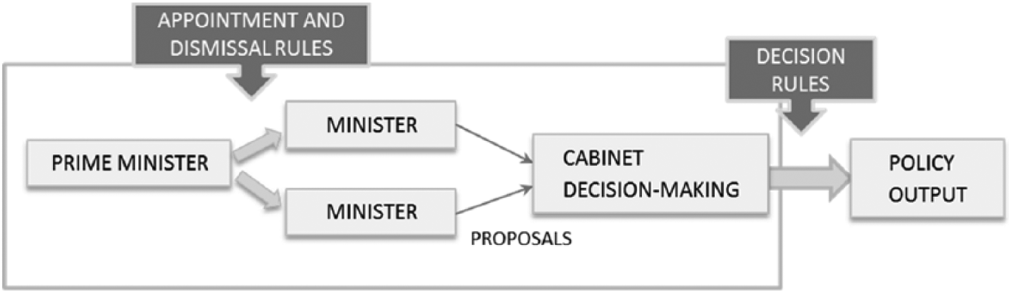
The Role of PM Powers Within the Policy-Making Process in Cabinets.

Bergman et al. (2003) also suggest that PM power is high when there is a constructive vote of no confidence, that is, when parliament is only allowed to withdraw confidence from a PM or cabinet if there is an absolute majority for a chosen successor. This rule was first implemented in Germany in order to avoid cabinet instability, but it is currently applied in several countries, for example, in Hungary and Spain (see, for example, Louwerse, 2014). Sartori (1994: 107) suggests that the effectiveness of the constructive vote “should not be sneezed at, for it is far easier to assemble a negative majority, a majority that simply ousts a government, than to bring together a positive majority that also agrees on the new chancellor.”

A related power of PMs focuses on the institutional feature of whether ministers can only be removed by parliament if the parliament dismisses the PM (ministers’ parliamentary accountability). In many countries, ministers can be directly held accountable by parliament (e.g. in Austria, Belgium, Denmark, and Sweden), whereas in others, they can only be dismissed if the PM is removed (e.g. in Germany and Spain; Bergman et al., 2003: 186–188).

We suggest that the two latter powers, the constructive vote of no confidence and ministers’ parliamentary accountability, operate in an indirect manner in influencing corruption, strengthening the PM’s power relative to the parliament, which, in turn, should influence the PM’s ability to appoint and dismiss ministers. When the parliament cannot simply dismiss a minister at will, the PM faces fewer constraints in staffing his or her cabinet. When a constructive vote of no confidence is needed to replace a cabinet, the PM is also directly strengthened in relation to the parliament, which we suggest should imply that the PM is less constrained in doing what he or she pleases when it comes to both staffing decisions in cabinet and making policy proposals.

To measure the constitutional powers of PMs, we rely on the European Representative Democracy Data Archive (http://www.erdda.se; Andersson et al., 2014), covering 29 European democracies (current EU member states except Croatia but including Iceland and Norway) from 1945 to 2013. Our test relies on a PM cabinet power index, which consists of (1) the existence of an actual decision rule for cabinet decision-making, such that the PM sums up the discussion or if majority voting applies (zero if cabinet decisions are made unanimously); whether the PM has the right to (2) appoint and (3) dismiss ministers; whether (4) ministers can only be removed by parliament if parliament dismisses the PM/full cabinet; and (5) a provision for constructive vote of no confidence, that is, whether parliament is only allowed to withdraw confidence from a PM/cabinet if there is an absolute majority for a chosen successor as PM (see Bergman et al., 2003: 157–167, 183–194).

The data for this 0–5 index are presented in Figure 2 for the 26 estimation sample countries (three countries are dropped due to lack of corruption data, see below). As expected, the German chancellor scores a maximum of 5, and also the Spanish PM wields equal powers. The UK PM, not being backed by the constructive vote of no confidence, scores a 4 at a level equal to Hungary. On the other side of the spectrum, Belgian, Finish, Italian, Latvian, and Dutch PMs are the weakest in relation to their cabinets. Only three countries have shifted powers over time, all in a positive direction: Belgium in 1995, Poland in 1997, and Finland in 2002.

Figure 2.

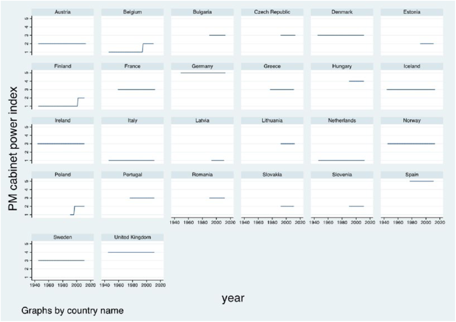
PM Powers in Sample Countries.

Measuring Corruption Perception

Our measure of corruption perception comes from the new Varieties of Democracy (V-Dem) dataset (Coppedge et al., 2016). The V-Dem data are primarily based on coding by five or more country experts, recruited on the basis of their local country-specific expertise, their seriousness of purpose, and impartiality. The data include expert perceptions of corruption and cover the entire globe from 1900 to 2012. In order to aggregate up from coders to the level of country-years, the V-Dem data are processed through an item response theory (IRT) measurement model that allows for both coder-specific reliability parameters and thresholds varying across coders (Pemstein et al., 2015). Through so-called “lateral” and “bridge” coding, meaning that a substantial number of coders also provide information for more than one country over time or for a particular year (2012), these measurement model estimates also attempt to correct for potential problems of incomparability across countries.

V-Dem includes perceptions of six distinct types of corruption that cover both different areas and levels of the polity realm, distinguishing between executive, legislative, and judicial corruption (see McMann et al., 2016 for exact details). Within the executive realm, the measures also distinguish between corruption mostly pertaining to bribery and corruption due to embezzlement. Finally, they differentiate between corruption in the highest echelons of the executive (at the level of the rulers/cabinet) on one hand, and in the public sector at large, on the other. The measures, thus, potentially tap into several distinguished types of corruption: both “petty” and ‘grand’, both bribery and theft, and both corruption aimed and influencing law making and that affecting implementation. But as shown by Kelly McMann et al. (2016), these measures are also strongly correlated, which based on principal component analysis warrants the construction of an overall factor index of corruption.

Although we are perfectly aware that there is no “gold standard” when it comes to measures of corruption, two features, thus, make the V-Dem corruption measures preferable to other extant measures, such as the Worldwide Governance Indicators measure of the Control of Corruption and the Corruption Perceptions Index produced by Transparency International, with which they are strongly correlated (at .85) in our estimation sample (see McMann et al., 2016). First, the possibility of disaggregating corruption into different sub-types provides a rare opportunity (not provided by the alternative indices) we take advantage of in a more refined test of our hypotheses. Second, by asking questions about corruption perceptions worded the same for each year going back to 1900, the V-Dem measures should allow comparisons over time for a hitherto unprecedentedly long-time series of corruption. This will prove critical for how we attempt to deal with the possibility of reversed causality (see below).

To allow readers the possibility to judge the face validity of the data themselves, the corruption index estimates are in Figure 4 presented in red for the in-sample years (for which there is also European Representative Democracy Data Archive (ERDDA) and in blue for the previous time periods of each country (mostly during authoritarianism or prior to World War II (WWII)). Since the underlying latent measurement model output is on a normal scale, the index, in principle, ranges from negative to positive infinity but, in practice, most of the variation in this sample ranges from −2 (less) to +1 (more corruption). As is well known from the previous literature on corruption in Europe (see, for example, Charron et al., 2013), there is both a North–South and an East–West divide in corruption levels, where more corrupt countries are located toward the East and the South. What Figure 4 also makes clear, and this is more news since corruption has never been measured over such an extensive period before, is that there is preciously little variation within countries over time. Corruption, much as its absence, is a very strong equilibrium. The more profound changes seem to concur with the out-of-sample transitions from authoritarianism to democracy.

One could, of course, question the precision of these expert perceptions of corruption levels in the past. However, we find the face validity of the historical trajectories of Figure 3 convincing. It should also be stressed that the multiple experts whose perceptions underlie the V-Dem scores are selected on the basis of their scholarly expertise, in this case with respect to the executive, legislature, and judiciary in each country. Their estimates are, thus, not based on vague guesses but based on the informed judgment (Schedler, 2012) of the nature of corrupt practices in the countries in question. Finally, McMann et al. (2016) show that, contrary to expectation, there is not more expert disagreement on these corruption variables further back in time, arguing that these estimates can, by and large, be considered reliable and valid.

Figure 3.

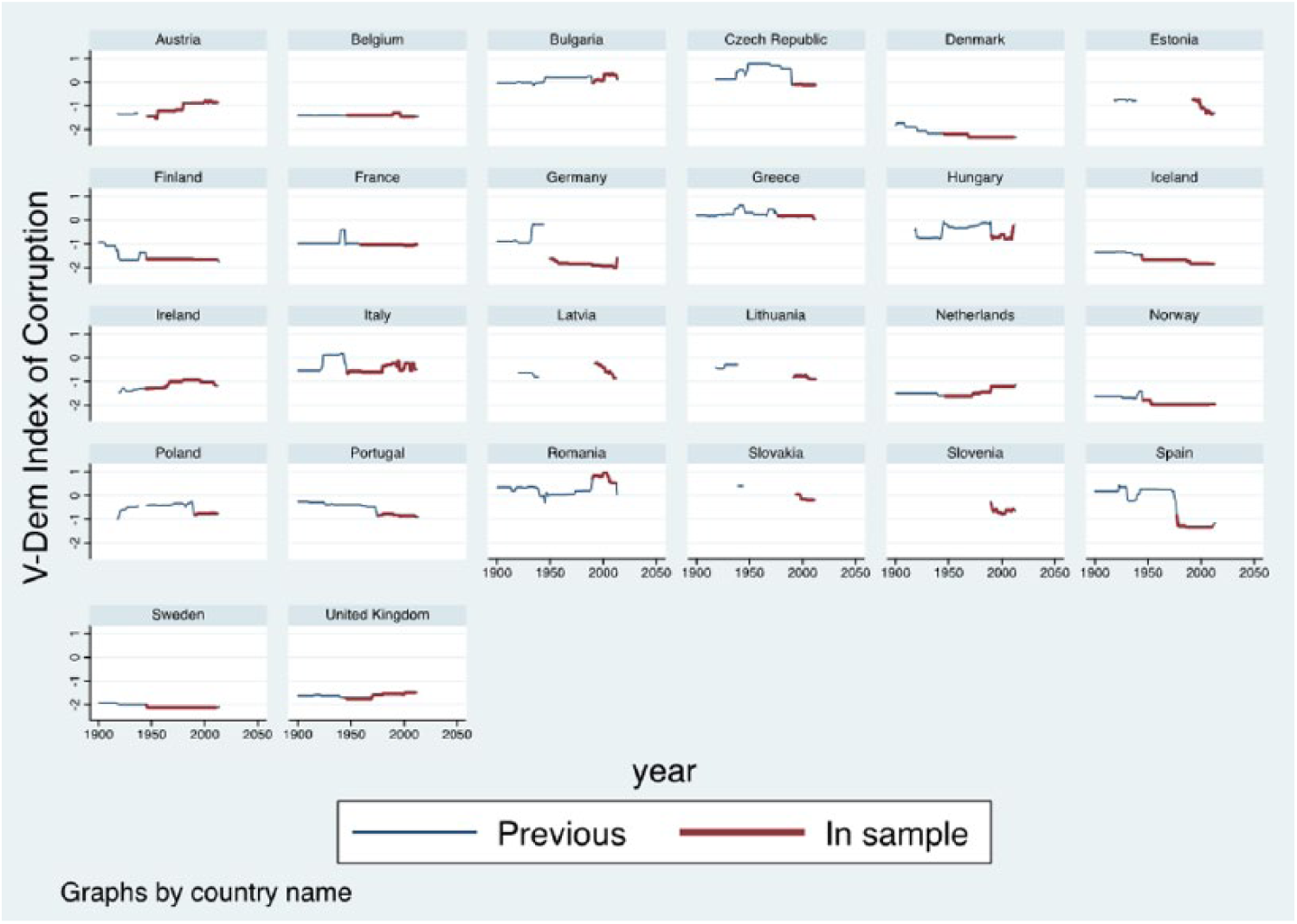
The Level of Corruption in Sample Countries.

Operationalization of Control Variables

Finally, drawing on the previous literature, we control for a series of other determinants of corruption that could potentially also be related to the powers of the PM. We include several variables focusing on cabinet and party system features, all drawn from the ERDDA-dataset (Andersson et al., 2014). We disaggregate the clarity of responsibility concept into its constitutive elements and estimate the effect of coalition and majority status separately, and also evaluate whether there is an interaction between majority and coalition status. We also control for oversized cabinet status (i.e. cabinets including one or more parties than necessary for majority status). Moreover, following Tavits (2007), we also test the effect of (logged) cabinet duration (in days), as well as the effective number of parties in the legislature.

Second, we control for a set of structural characteristics well known to be related to corruption: ln(GDP/capita); the level of democracy; a dummy for post-communist countries, known to have a stronger and very different legacy of corruption; the share of protestants in the population; and the degree of ethnic fractionalization. Except for the level of democracy, measured by the V-Dem index of polyarchy (Coppedge et al., 2015), data on these structural variables have been drawn from the QoG dataset (Teorell et al., 2015).

As a third set of controls, we also include measures of two potential institutional determinants of corruption: a dummy for semi-presidentialism (from the ERDDA described above) and two features of the electoral system in use, the (logged) average district magnitude and a dummy for whether proportional representation (PR) or a mixed majoritarian/PR formula was in use (data from Bormann and Golder, 2013). We also control for the cabinet preference range (the ideological distance on a left–right dimension between the parties to the “extremes” in a cabinet), since some scholars have suggested that ideologically cohesive cabinets can be expected to be less corrupt (see Strøm et al., 2003: 726).²

Empirical Analysis

In combining the ERDDA with V-Dem data, our estimation sample consists of a maximum of 26 European democracies from 1945 to 2012.³ Given the pooled time-series cross-section structure of our data, in combination with the slow-moving nature of dependent and independent variables, we present a wide array of estimators to assess our hypothesis. We, thus, fully acknowledge the uncertainty inherent in these data and the inferences from our estimation strategy. Due to data limitations, one should interpret our results more as a serious plausibility probe than as a conclusive test of our theory. In the following part, we present an analysis of the entire sample, which is followed by a more in-depth study of the Belgian case.

Analyzing the Relationship Between PM Powers and Corruption in Europe

We start in Figure 4 by presenting the most simple descriptive portrayal or the relationship between corruption and PM powers: a scatterplot with a locally weighted regression line. Confirming our expectation, there is a general tendency that with more PM cabinet powers, levels of corruption are lower. Although suggestive evidence in itself, this picture does not take time, the direction of causality, autocorrelation, or potential confounders into account.

Figure 4.

The Level of Corruption and PM Cabinet Power.

In Table 1, we therefore introduce the full set of control variables. The eight different models to varying agrees exploit the cross-sectional versus over-time variation in the data. All models are run with and without a control for the “corruption legacy” of each country. Referring back to Figure 3, this variable takes the average of a country’s corruption level from the year 1900 (or the first year of appearance in the V-Dem data) up until the year in which it first enters our estimation sample.⁴ The purpose of this control is to mitigate reverse causality bias, that is, the possibility that countries facing serious problems with corruption historically were also the ones introducing constitutional and other safeguards for strengthening the powers of the PM vis-à-vis the cabinet.

Table 1.

The Power of Prime Ministers and Corruption.

	(1)	(2)	(3)	(4)	(5)	(6)	(7)	(8)
	Cross-sectional	Cross-sectional	5-year averages	5-year averages	Pooled	Pooled	Prais–Winsten PCSEs	Prais–Winsten PCSEs
PM cabinet power index	–0.0452(0.1939)	–0.3114(0.1759)	–0.0570(0.0383)	–0.1708***(0.0395)	–0.0739***(0.0177)	–0.1647***(0.0146)	–0.0904***(0.0140)	–0.0929***(0.0153)
Corruption legacy		0.5551**(0.2050)		0.4983***(0.0556)		0.4994***(0.0209)		0.4970***(0.0368)
Rho (ρ)	–	–	–	–	–	–	0.923	0.957
R ²	0.889	0.948	0.762	0.847	0.752	0.845	0.707	0.707
Observations	26	26	221	221	974	974	974	974

Entries are regression coefficients with standard errors within parentheses (in models 7 and 8 panel corrected with Prais–Winsten-autocorrelated errors).

PCSE: panel-corrected standard errors

p < 0.10, ^**p < 0.05, ^***p < 0.01.

The results show consistent support for the argument that PM cabinet powers reduce corruption. All estimated coefficients for our variable of interest are negative but not all are statistically significant. In the purely cross-sectional models 1 and 2, based on 26 observations and with all over-time variation taken out of the data, the noise simply overwhelms the signal. When we turn to models 3 and 4 based on data averaged over 5-year periods, which gives us roughly eight times more observations, we find a significant effect with the legacy control in place but not without it. In the pooled country-year-level models 5 and 6, the number of observations increase to 974 and the signal-to-noise ratio is such that the result is clearly significant in both specifications. But with so little over-time variation in both the dependent and independent variables, the pooled models arguably exaggerate the true number of independent observations. A cautious balance between the two extremes (n = 26 and n = 974), but based on a measure of the level of over-time dependence (autocorrelation) rather than the arbitrary 5-year bins, is presented in models 7 and 8. This is still a pooled model but with the standard errors corrected for not only serial correlation, which is substantial (rho is above 0.90), but also for panel heteroskedasticity and spatial autocorrelation. In other words, here, we rely on the standard Nathaniel Beck and Jonathan Katz’s (1995) panel-corrected standard errors. Our results are still in the expected direction and statistically significant.

The relationship between PM powers and corruption, taking all control variables into account (model 8 of Table 1), is portrayed in Figure 5. Figure 5(a) displays the relationship for the full estimation sample. In concrete terms, every addition of one type of power to the PM cabinet power index leads, all else equal, to an expected average reduction in the level of corruption by −0.0929. Since the figure seems to indicate the influence of a few extreme outliers, notably the three cases of change (Belgium in 1995, Poland in 1997, and Finland in 2002), and also cases such as Germany in 1991 and Spain in 1977, we re-estimated the relationship after having dropped the (15%) most influential outliers, resulting in the narrower sample of country years in Figure 5(b). As can be seen, the conditional effect of PM powers is strengthened once these influential outliers are eliminated.

Figure 5.

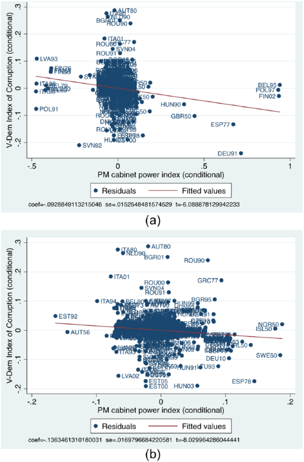
The Conditional Effect of PM Powers (a) Including and (b) Excluding Outliers.

In Table 2, we evaluate our main hypothesis against two types of corruption, roughly corresponding to the two different branches of government downstream of the PM represented in the ‘chain of delegation’: the cabinet ministers and the “civil servants” in the public sector at large. For comparative purposes, we include the final two models of Table 1, with the overall corruption index, but in models 3–6 we, instead, include tests differentiating between “grand” corruption (only including bribery and embezzlement within the highest echelons of the executive) and “bureaucratic” corruption, including the same types of malfeasance among bureaucrats in the public sector at large. The proposition most obviously related to our theory is that cabinet or “grand” corruption should be most directly affected by the authority of the PM. We have less clear expectations when it comes to corruption in the public sector at large, but if accountability in the third step in the chain, between PMs and minister, also translates into the fourth one, between ministers and civil servants, we can expect the same general effects on “petty” corruption. Since the legislature is located before the PM in the delegation chain, we do not expect any effects on legislative corruption.

Table 2.

Types of Corruption.

	(1)	(2)	(3)	(4)	(5)	(6)
	Overall	Overall	Grand	Grand	Bureaucratic	Bureaucratic
PM cabinet power index	–0.0904***	–0.0929***	–0.0513***	–0.0663***	–0.0141	–0.0766***
	(0.0140)	(0.0153)	(0.0186)	(0.0211)	(0.0129)	(0.0151)
Corruption legacy		0.4970***
		(0.0368)
Grand corruption legacy				0.1764***
				(0.0540)
Bureaucratic corruption						0.4815***
legacy						(0.0390)
Executive corruption					0.4626***	0.3218***
					(0.0429)	(0.0445)
Bureaucratic corruption			0.3107***	0.2701***
			(0.0421)	(0.0479)
Legislative corruption			0.2022***	0.1884***	0.0901***	0.0142
			(0.0251)	(0.0264)	(0.0258)	(0.0257)
Majority cabinet	0.0019	0.0001	0.0030	0.0025	0.0037	0.0001
	(0.0061)	(0.0049)	(0.0081)	(0.0080)	(0.0093)	(0.0078)
Coalition cabinet	0.0033	0.0058	0.0130	0.0134	–0.0198*	–0.0094
	(0.0073)	(0.0057)	(0.0088)	(0.0087)	(0.0103)	(0.0087)
Oversized cabinet	0.0131**	0.0128**	0.0011	0.0024	0.0011	0.0071
	(0.0064)	(0.0054)	(0.0083)	(0.0083)	(0.0095)	(0.0086)
ln(cabinet duration)	0.0006	0.0012	0.0030	0.0031	0.0005	0.0015
	(0.0029)	(0.0021)	(0.0032)	(0.0031)	(0.0042)	(0.0036)
Effective number of parties	–0.0093*	–0.0067*	–0.0007	–0.0007	–0.0058	–0.0039
	(0.0051)	(0.0035)	(0.0055)	(0.0053)	(0.0059)	(0.0051)
Cabinet preference range	–.00003**	–0.0003**	–0.0005***	–0.0005***	0.0001	0.0000
	(0.0002)	(0.0001)	(0.0002)	(0.0002)	(0.0002)	(0.0002)
ln(Gdp/cap)	–0.0086	–0.0227	0.0861**	0.0776**	–0.0672**	–0.0673***
	(0.0248)	(0.0269)	(0.0338)	(0.0338)	(0.0262)	(0.0261)
Level of democracy	–.07717***	–0.6626***	–0.4270***	–0.4742***	–0.1267	–0.1465
	(0.0975)	(0.0944)	(0.1206)	(0.1239)	(0.1512)	(0.1254)
Post-communist	0.8118***	0.2942***	0.3657***	0.2131***	0.3729***	–0.0985*
	(0.0477)	(0.0579)	(0.0756)	(0.0745)	(0.0652)	(0.0523)
Religion: protestant	–0.0111***	–0.0066***	–0.0016**	–0.0013*	–0.0065***	–0.0055***
	(0.0005)	(0.0007)	(0.0008)	(0.0007)	(0.0006)	(0.0005)
Ethnic fractionalization	–0.6272***	–0.6526***	–0.6914***	–0.7878***	–0.0548	–0.5485***
	(0.1426)	(0.1733)	(0.1757)	(0.1795)	(0.1086)	(0.1062)
Semi-presidential system	–0.0168	–0.0421**	–0.0409	–0.0561**	0.0739***	–0.0175
	(0.0352)	(0.0182)	(0.0285)	(0.0269)	(0.0254)	(0.0178)
ln(district magnitude)	–0.0387***	–0.0443***	–0.0844***	–0.0874***	0.0359***	0.0152
	(0.0099)	(0.0095)	(0.0136)	(0.0138)	(0.0138)	(0.0125)
PR/mixed	0.1537***	0.0884***	0.1853***	0.1764***	0.0636*	–0.0386
	(0.0263)	(0.0217)	(0.0314)	(0.0318)	(0.0329)	(0.0290)
Constant	0.0937	0.6110**	–0.8722***	–0.Ֆ9*	0.3301	0.9551***
	(0.2577)	(0.2668)	(0.3332)	(0.3290)	(0.2723)	(0.2628)
Rho (ρ)	0.923	0.957	0.933	0.933	0.870	0.899
R ²	0.707	0.707	0.666	0.670	0.742	0.753
Number of countries	26	26	26	26	26	26
Average number of years/country	37.5	37.5	37.5	37.5	37.5	37.5
Observations	974	974	974	974	974	974

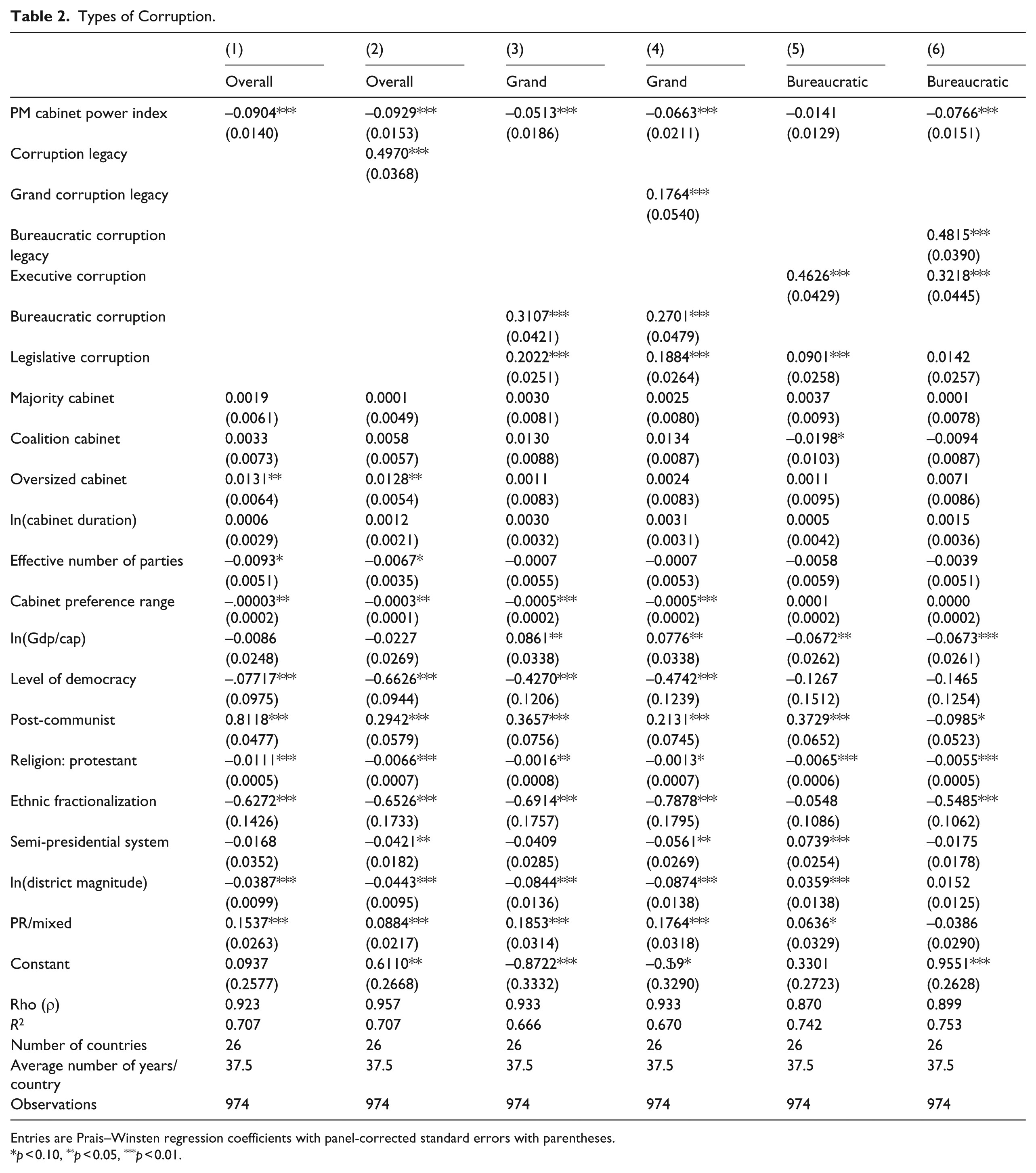
Entries are Prais–Winsten regression coefficients with panel-corrected standard errors with parentheses.

p < 0.10, ^**p < 0.05, ^***p < 0.01.

To test for these claims, we must not only look at different types of corruption as dependent variables but also control for the other respective types in each regression. The reason for this is that, corruption being a systemic phenomenon, the different types of corruption are generally very highly correlated (at around 0.86 in the estimation sample). In order to purge the estimates of the effect on one type from the effect on the other, the other types must, thus, be controlled for. In line with expectations, PM powers reduce both grand and bureaucratic corruption, particularly when we control for the historical legacy of such corruption. There, thus, seems to be something to the chain of delegation that goes beyond the cabinet as such (and beyond the indirect pathway passing through grand corruption) that equips a strongly positioned PM with powers to also reduce corruption in the public sector at large.

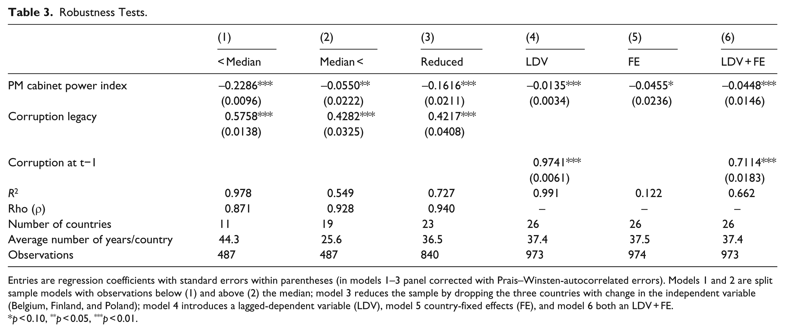
We also conduct a series of robustness tests (see also Table 3 in Appendix 1). Given the large variation in levels of corruption across Europe, we start by running a split sample test, separating country year below (model 1) and above (model 2) the sample median. We then take another precaution against potentially influential extreme outliers by excluding the three countries that experience change in the PM powers index (Belgium, Finland, and Poland). This model 3 is, thus, purely based on cross-sectional variation, but pooled across all countries and years. With the same overall estimator in place (Prais–Winsten PCSEs), our main result remains robust. In the final three robustness tests, we shift to the opposite strategy, only exploiting the over-time variation in the data. Model 4 includes a lagged dependent variable, tantamount to turning the dependent variable into (yearly) change in levels of corruption. Model 5, instead, introduces country-fixed effects, turning the explanatory focus exclusively into variation within countries over time. Model 6, finally, includes both, thus, restricting attention to change within countries over time. Our overall result holds, although it is only marginally significant with the fixed-effects estimator.

A Controlled Comparison of the Case of Belgium

As a final test of our theoretical proposition, we conduct a controlled comparison of the case of Belgium, where a constructive vote of no confidence was introduced in 1995 (De Winter and Dumont 2003: 260). According to the literature, and in accordance with our measurement strategy, this served to strengthen the position of the Belgian PM (Fiers and Krouwel, 2005: 129). But did it impact on corruption? As apparent already in Figure 3, there is an increase in perceived corruption levels in Belgium in the early 1990s, followed by a drop toward the end of the decade. This is largely consistent with both qualitative and quantitative evidence of corruption levels in Belgium, where both public perceptions and judicial statistics point at the 1990s as a particularly corrupt decade (De Winter, 2003; Maesschalk and Van De Walle, 2006). While our theory cannot account for the rise in corruption in Belgium, this is still evidence indicative of a downward shift following the strengthening of PM powers.

Applying the synthetic control method (Abadie et al., 2014), we can even estimate the approximate size of the effect in Belgium, while controlling for the same set of covariates as in our regression-based estimates above.⁵ Although no singular case can perfectly replicate the relevant counter-factual—that is, a Belgium without the introduction of a constructive vote of confidence—Alberto Abadie et al. (2014) provide a method for finding a weighted combination of other cases that can reproduce the characteristics of the treatment case, thus providing a “synthetic control” against which the treatment effect in a case can be estimated. After feeding this algorithm with a “donor pool” of other countries with characteristics similar to the treated unit (here, all non-postcommunist countries that did not experience the treatment, excluding Finland), the synthetic control group in our case consists of a weighted average of Ireland (0.190), Italy (0.288), Denmark (0.327) and Iceland (0.195; with their relative weights provided in parentheses).⁶

Figure 6 plots the corruption scores for Belgium and this synthetic control group over the 1977–2003 time period common to all countries in the “donor pool,” with the treatment in 1995 highlighted by the diagonal red line. As can be seen, there is a fairly good fit between the two lines pre-treatment,⁷ indicating that the synthetic control group should be able to proxy for the development of Belgium in the counter-factual scenario with no exposure to the strengthening of PM powers. While the lines track each other for a couple of years also post-treatment, indicating little of a short-run effect, they diverge from 2001 onward and stabilizes at a difference of −0.0705. Reassuringly, this is an estimate of the long-run effect very similar in magnitude to our regression estimates based on the full estimation sample.

Figure 6.

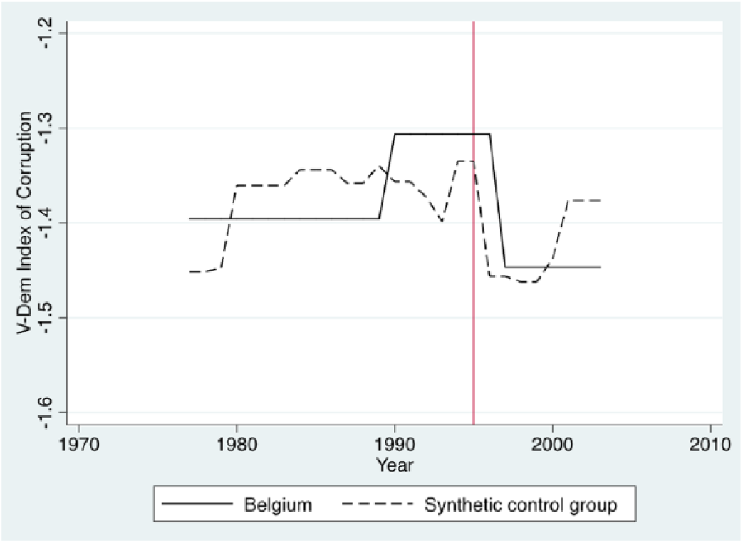
Trends in Corruption: Belgium vs. Synthetic Control Group.

Concluding remarks

The aim of this article has been to contribute to the literature, explaining high-level corruption in parliamentary systems. Drawing on the literature on coalition governance, we suggest that the ability of key political actors, as principals, to control the agents that have been delegated power in cabinet should matter for limiting corruption. Using a new measure of corruption from the Varieties of Democracy data, our results show that corruption is significantly lower in countries where the PM has strong constitutional powers. Given the slow-moving nature of both corruption and PM powers, our empirical results should be interpreted as suggestive. Future work should investigate into PM powers over time for a larger sample of countries, allowing for more conclusive tests that can rely on within-country variation over time.

As mentioned, a number of control mechanisms have been seen as solutions to potential problems of “agency loss” that arise when power is delegated to individual ministers. In this article, we have focused on the role of the PM in controlling “ministerial drift” and corruption, also finding some support for this idea. This suggests that a focus on coalition governance mechanisms in controlling corruption is fruitful, and we, thus, propose that future research should study the role of other such mechanisms, for example, by investigating the impact of the appointment of “junior watchdog ministers” (e.g. Thies, 2001) on the level of corruption. If a junior minister from another party other than the Head of Department is appointed to “keep tabs” on the minister, this could clearly limit corruption, as the “watchdog” can inform the PM of any potential malpractice in the department.

Theoretically, our argument is based on the assumption that the PM has an interest in reducing corruption within the cabinet and among his or her ministers, since the PM has an interest in implementing a specific policy program. The fact that our theoretical expectation seems to be borne out in itself supports this assumption, but we readily admit that there is most likely great variation between PMs with respect to their incentives to combat corruption. A question to be addressed in future work is when we might expect such “good” principals, or more specifically PMs, who have an interest in achieving a non-corrupt cabinet?

A natural extension of our argument would seem to be that presidents, who typically wield strong powers over their respective cabinets, should achieve lower corruption levels. However, here, we know from the previous empirical literature on corruption that presidential systems are typically associated with higher levels of corruption (see, for example, Gerring et al., 2009). We can only speculate about why our argument might not transfer from parliamentary to presidential systems, but there may be other institutional reasons for expecting parliamentary systems to perform better than their presidential counterparts, having less to do with the power of political leaders and having more to do with the simplicity and indirectness of the parliamentary chain of delegation (Strøm, 2003). This could increase the incentives for principals to monitor and control agents, which could explain why parliamentary systems perform better. This is another important topic worthy of further study.

Footnotes

Appendix 1

Table 3.

Robustness Tests.

	(1)	(2)	(3)	(4)	(5)	(6)
	< Median	Median <	Reduced	LDV	FE	LDV + FE
PM cabinet power index	–0.2286***	–0.0550**	–0.1616***	–0.0135***	–0.0455*	–0.0448***
	(0.0096)	(0.0222)	(0.0211)	(0.0034)	(0.0236)	(0.0146)
Corruption legacy	0.5758***	0.4282***	0.4217***
	(0.0138)	(0.0325)	(0.0408)

Corruption at t−1				0.9741***		0.7114***
				(0.0061)		(0.0183)
R ²	0.978	0.549	0.727	0.991	0.122	0.662
Rho (ρ)	0.871	0.928	0.940	–	–	–
Number of countries	11	19	23	26	26	26
Average number of years/country	44.3	25.6	36.5	37.4	37.5	37.4
Observations	487	487	840	973	974	973

Entries are regression coefficients with standard errors within parentheses (in models 1–3 panel corrected with Prais–Winsten-autocorrelated errors). Models 1 and 2 are split sample models with observations below (1) and above (2) the median; model 3 reduces the sample by dropping the three countries with change in the independent variable (Belgium, Finland, and Poland); model 4 introduces a lagged-dependent variable (LDV), model 5 country-fixed effects (FE), and model 6 both an LDV + FE.

p < 0.10, ^**p < 0.05, ^***p < 0.01.

Acknowledgements

We are very grateful for the help provided by Torbjörn Bergman, Svante Ersson, and Holger Döring, and for the excellent research assistance provided by Talib Jabbar. Hanna Bäck and Jan Teorell carried out most of the work on this article and should be given the main credit for it.

Funding

The author(s) disclosed receipt of the following financial support for the research, authorship, and/or publication of this article: This research was supported by Riksbankens Jubileumsfond [Grant M14-0087:1]; by Riksbankens Jubileumsfond [Grant M13- 0559:1], by the Swedish Research Council [Grant C0556201]; and by the Knut and Alice Wallenberg Foundation [Grant 2013.0166].

Notes

ORCID iD

Hanna Bäck

Author Biographies

Hanna Bäck is a Professor of Political Science at Lund University, Sweden. Her research concentrates mainly on political parties and coalition politics in parliamentary democracies, focusing on coalition formation, portfolio allocation, cabinet reshuffles, and policy-making in multiparty governments.

Jan Teorell is a Professor of Political Science at Lund University, Sweden. He is one of the creators of the Quality of Government and V-Dem datasets. His research concentrates mainly on history and comparative politics, comparative democratization, corruption, and state-making.

Staffan I. Lindberg is a Professor of Political Science at University of Gothenburg, Sweden. He is the Director of the V-Dem Institute at University of Gothenburg. His research concentrates mainly on democracy and democratization, African politics, corruption and clientelism.

References

Abadie

Diamond

Hainmueller

(2014) Comparative Politics and the Synthetic Control Method. Journal of the American Statistical Association 105 (490): 493–505.

Andersson

Bergman

Ersson

(2014) The European Representative Democracy Data Archive, Release 3. Stockholm: Riksbankens Jubileumsfond.

Bäck

Hadenius

(2008) Democracy and State Capacity: Exploring a J-shaped Relationship. Governance 21: 1–24.

Bäck

Debus

Müller

(2016) Intra-Party Diversity and Ministerial Selection in Coalition Governments. Public Choice 166: 355–378.

Bardhan

(1997) Corruption and Development: A Review of Issues. Journal of Economic Literature 35 (3): 1320–1346.

Beck

Katz

(1995) What to do (and not to do) with Time-Series Cross-Section Data. American Political Science Review 89: 634–647.

Bergman

Müller

Strøm

et al . (2003) Democratic Delegation and Accountability: Cross-National Patterns. In: Strøm

Müller

Bergman

(eds) Delegation and Accountability in Parliamentary Democracies. Oxford: Oxford University Press, pp.109–220.

Bormann

N-C

Golder

(2013) Democratic Electoral Systems Around the World, 1946–2011. Electoral Studies 32 (2): 360–369.

Carroll

Cox

(2012) Shadowing Ministers Monitoring Partners in Coalition Governments. Comparative Political Studies 45 (2): 220–236.

10.

Charron

Lapuente

Rothstein

(2013) Quality of Government and Corruption from a European Perspective: A Comparative Study on the Quality of Government in EU Regions. Cheltenham: Edward Elgar Publishing.

11.

Coppedge

Gerring

Lindberg

et al . (2015) Varieties of Democracy: Dataset v4. Varieties of Democracy (V-Dem) Project. Available at: www.v-dem.net

12.

Coppedge

Gerring

Lindberg

et al . (2016) V-Dem Country-Year Dataset v6.2. Varieties of Democracy (V-dem) Project. Available at: https://www.v-dem.net/en/data/data-version-6-2/

13.

De Winter

(2003) Political Corruption in Belgium. In: Bull

Newell

(eds) Corruption in Contemporary Politics. Basingstoke: Palgrave Macmillan, pp.93–105.

14.

De Winter

Dumont

(2003) Belgium: Delegation and Accountability under Partitocratic Rule. In: Strøm

Müller

Bergman

(eds) Delegation and Accountability in Parliamentary Democracies. Oxford: Oxford University Press, pp.253–280.

15.

Fiers

Krouwel

(2005) The Low Countries: From “Prime Minister” to President-Minister. In: Poguntke

Webb

(eds) The Presidentialization of Politics: A Comparative Study of Modern Democracies. Oxford: Oxford University Press, pp.128–158.

16.

Gerring

Thacker

Moreno

(2009.) Are Parliamentary Systems Better? Comparative Political Studies 42 (3): 327–359.

17.

Groenendijk

(1997) A principal-Agent Model of Corruption. Crime, Law and Social Change 27 (3–4): 207–229.

18.

Hallerberg

Von Hagen

(1999) Electoral Institutions, Cabinet Negotiations, and Budget Deficits n the European Union. In: Poterba

Von Hagen

(eds) Fiscal Institutions and Fiscal Performance. Chicago, IL: University of Chicago Press, pp.209–232.

19.

Huber

Martínez-Gallardo

(2008) Replacing Cabinet Ministers: Patterns of Ministerial Stability in Parliamentary Democracies. American Political Science Review 102 (2): 169–180.

20.

Indridason

Kam

(2008) Cabinet Reshuffles and Ministerial Drift. British Journal of Political Science 38 (4): 621–656.

21.

Kam

Bianco

Sened

et al . (2010) Ministerial Selection and Intraparty Organization in the Contemporary British Parliament. American Political Science Review 104 (2): 289–306.

22.

Kam

Indridason

(2005) The Timing of Cabinet Reshuffles in Five Westminister Parliamentary Systems. Legislative Studies Quarterly 30 (3): 327–364.

23.

King

(1994) Chief Executives in Western Europe. In: Budge

McKay

(eds) Developing Democracy: Comparative Research in Honour of J F P Blondel. London: SAGE Publishing, pp.150–163.

24.

Klitgaard

(1988) Controlling Corruption. Berkeley, CA: University of California Press.

25.

La Porta

Lopez-de-Silanes

Shleifer

et al . (1999) The Quality of Government. The Journal of Law, Economics, and Organization 15 (1): 222–279.

26.

Louwerse

(2014) Unpacking “Positive” and “Negative” Parliamentarism. Paper Presented at the ECPR Joint Sessions, Salamanca, 10–15 April.

27.

McMann

Pemstein

Seim

et al . (2016) Strategies of Validation: Assessing the Varieties of Democracy Corruption Data. V-Dem Institute, Working Paper Series 2016:23, February. Gothenburg: University of Gothenburg.

28.

Maesschalk

Van De Walle

(2006) Policy Failure and Corruption in Belgium: Is Federalism to Blame? West European Politics 29 (5): 999–1017.

29.

Martin

Vanberg

(2011) Parliaments and Coalitions: The Role of Legislative Institutions in Multiparty Governance. Oxford: Oxford University Press.

30.

Müller

Strøm

(2000) Conclusion. In: Müller

Strøm

(eds) Coalition Governments in Western Europe. Oxford: Oxford University Press, pp.559–592.

31.

Müller

Strøm

(2008) Coalition Agreements and Cabinet Governance. In: Strøm

Müller

Bergman

(eds) Cabinet Governance: Bargaining and the Cycle of Democratic Politics. Oxford: Oxford University Press, pp.159–199.

32.

O’Malley

(2007) The Power of Prime Ministers: Results of an Expert Survey. International Political Science Review 28 (1): 7–27.

33.

Pemstein

Marquardt

Tzelgov

et al . (2015) The V-Dem Measurement Model: Latent Variable Analysis for Cross-National and Cross-Temporal Expert-Coded Data. V-Dem Institute, Working Paper Series 2015: 21, December. Gothenburg: University of Gothenburg.

34.

Persson

Rothstein

Teorell

(2013) Why Anticorruption Reforms Fail—Systemic Corruption as a Collective Action Problem.” Governance: An International Journal of Policy, Administration and Institutions 26: 449–471.

35.

Powell

(2000) Elections as Instruments of Democracy. New Haven, CT: Yale University Press.

36.

Rose-Ackerman

(1978) Corruption: A Study in Political Economy. New York: Academic Press.

37.

Rose-Ackerman

(1999) Corruption and Government: Causes, Consequences, and Reform. Cambridge: Cambridge University Press.

38.

Sartori

(1994) Comparative Constitutional Engineering. London: Palgrave Macmillan.

39.

Schedler

(2012) Judgment and Measurement in Political Science. Perspectives on Politics 10 (1): 21–36.

40.

Schwindt-Bayer

Tavits

(2016) Clarity of Responsibility, Accountability, and Corruption. Cambridge: Cambridge University Press.

41.

Strøm

(2003) Parliamentary Democracy and Delegation. In: Strøm

Müller

Bergman

(eds) Delegation and Accountability in Parliamentary Democracies. Oxford: Oxford University Press.

42.

Strøm

Müller

Bergman

(eds) (2003) Delegation and Accountability in Parliamentary Democracies. Oxford: Oxford University Press.

43.

Strøm

Müller

Smith

(2010) Parliamentary Control of Coalition Governments. Annual Review of Political Science 13: 517–535.

44.

Tavits

(2007) Clarity of Responsibility and Corruption. American Journal of Political Science 51: 218–229.

45.

Teorell

Dahlberg

Holmberg

et al . (2015) The Quality of Government Standard Dataset (Version 15 January). Gothenburg: The Quality of Government Institute, University of Gothenburg. Available at: http://www.qog.pol.gu.se

46.

Thies

(2001) Keeping Tabs on Partners: The Logic of Delegation in Coalition Governments. American Journal of Political Science 45 (3): 580–598.

47.

Treisman

(2007) What Have We Learned About the Causes of Corruption from Ten Years of Cross-National Empirical Research? Annual Review of Political Science 10: 211–244.