Fiscal Policy and Monetary Integration in the Ecowas

Abstract

Those with dissenting view regarding the structure of monetary union arrangement in ECOWAS often argue that the macroeconomic convergence criteria have hampered the ability of countries in the region to stabilize their economies with appropriate counter-cyclical fiscal policy. We test the empirical merit of this assertion and found no support for this view. Instead, discretionary fiscal policy has actually become counter-cyclical in ECOWAS after the introduction of convergence criteria. In specifics, we found a switch from pro-cyclical fiscal policymaking in the pre-convergence era (1995–2002) to a counter-cyclical fiscal policymaking in the convergence era (2003–2018) in ECOWAS, and that policymakers in the region respond to initial conditions - apparently taking clue from past (initial) debt and past deficit. The policy import of our result is the need to: (i) introduce more flexibility in fiscal policymaking through discretionary fiscal policy that balances the budget (against the constraints imposed by the convergence rules) over the business cycle; and (ii) adopt ‘discretionary fiscal deficit’ to monitor compliance (rather than gross deficit) because it represents effort made to correct excess deficit.

Keywords

discretionary fiscal policy monetary integration ECOWAS

Introduction

The fiscal apparatus of the convergence criteria in the ECOWAS sub-region – modeled after the Maastricht fiscal policy rules and the Stability and Growth Pact (SGP) – is increasingly being regarded as an unnecessary straightjacket on national fiscal policy. It is argued – by some dissenting viewpoint (see e.g., Saka et al., 2015) - that this could weaken the ability and/motivation of ECOWAS countries to stabilize their economies through active countercyclical fiscal policy.¹ While it is fairly clear that discretionary fiscal policy is useful for stabilizing business cycle fluctuations, the problem here is that if the presumption of the dissenting viewpoint is true, this could have long-run consequences on the investment and growth potential of the ECOWAS economies that go well beyond their implications for the cyclical properties of fiscal policy.

This argument seems to have gained momentum after it became clear that many WAMZ and WAEMU economies have rather been unable to meet and sustain the convergence criteria despite clear attempts to implement the rules in the respective economies.² The reasoning is that the satisfaction of the convergence criteria – an indication of shock synchronization under a common monetary policy– is a precondition for a successful launch of a common currency. Over the past one and a half decades (2004–2018), there isn’t any single year for which either the entire WAMZ (six) or WAEMU (eight) countries were able to satisfy the (total) fiscal deficit criterion.³ Considering the 14 ECOWAS countries as a group, the best performing year over the 15 years period (2004–2018) was in 2007 when 7 out of the 14 ECOWAS countries managed to satisfy this criterion (Table 2). This situation is more disturbing particularly for WAMZ countries where all Member States have persistently failed to meet this criterion over the preceding four consecutive years (2014–2018). While these developments have led to dissenting views and recurring postponement of the launch of the proposed single currency in the region (now scheduled for 2020), a number of contemporary researchers have argued for fiscal policy flexibility that is tied to business cycles (see e.g., Debrun et al., 2005; Wyplosz, 2002; Wyplosz, 2005).

Table 2.

Highlight of ECOWAS Compliance Level on the Convergence Criteria Pendulum:.

s/no	Converg. Criteria	Summary of Performance	No of WAMZ countries satisfying criteria (yrs)	No of WAEMU countries satisfying criteria (yrs)
1	Fiscal Deficit Cri.	ECOWAS, as a sub-region, performed abysmally poor on fiscal deficit criterion.	4 (2007)	4 (2005)
2	Months of import criterion	WAEMU surpassed the benchmark consistently over the entire review period of 1995–2018 while WAMZ persistently failed to meet the criterion. The situation for WAEMU is understandably clear given that the elimination of exchange rate risk (via the CFA-euro peg) also eliminates or, at least, reduces the risk of a balance of payment crisis. This helped ensured that the WAEMU economies are able to build sufficient foreign reserve needed to meet this convergence criterion	4 (2014)	8 (2002–18)
3	Growth rate criterion	WAEMU has never been able to meet the 7% growth benchmark notwithstanding the recent impressive growth scorecard of Cote d’Ivoire. WAMZ managed to meet this criterion only twice in 2012 & 2013. Prior to 2014, WAMZ surpassed WAEMU on growth criterion led mainly by high growth in Nigeria and Sierra Leone.	3 (2012, 2013	1 (2013–18)
4	Inflation Criterion	The absence of exchange rate risk (made possible by the CFA-euro peg) is associated with low inflation in WAEMU. Thus, over the entire 10-year period, all 8 WAEMU countries satisfied and sustained the inflation criterion. On the other hand, the WAMZ countries have never met this criterion as a group since the convergence criteria were adopted in 2002.	0 (2005–18)	8 (2005–18)
5	Debt: Outstanding domestic and external debt/GDP ≤ 70	ECOWAS did not also do well on the debt criterion.	-	-

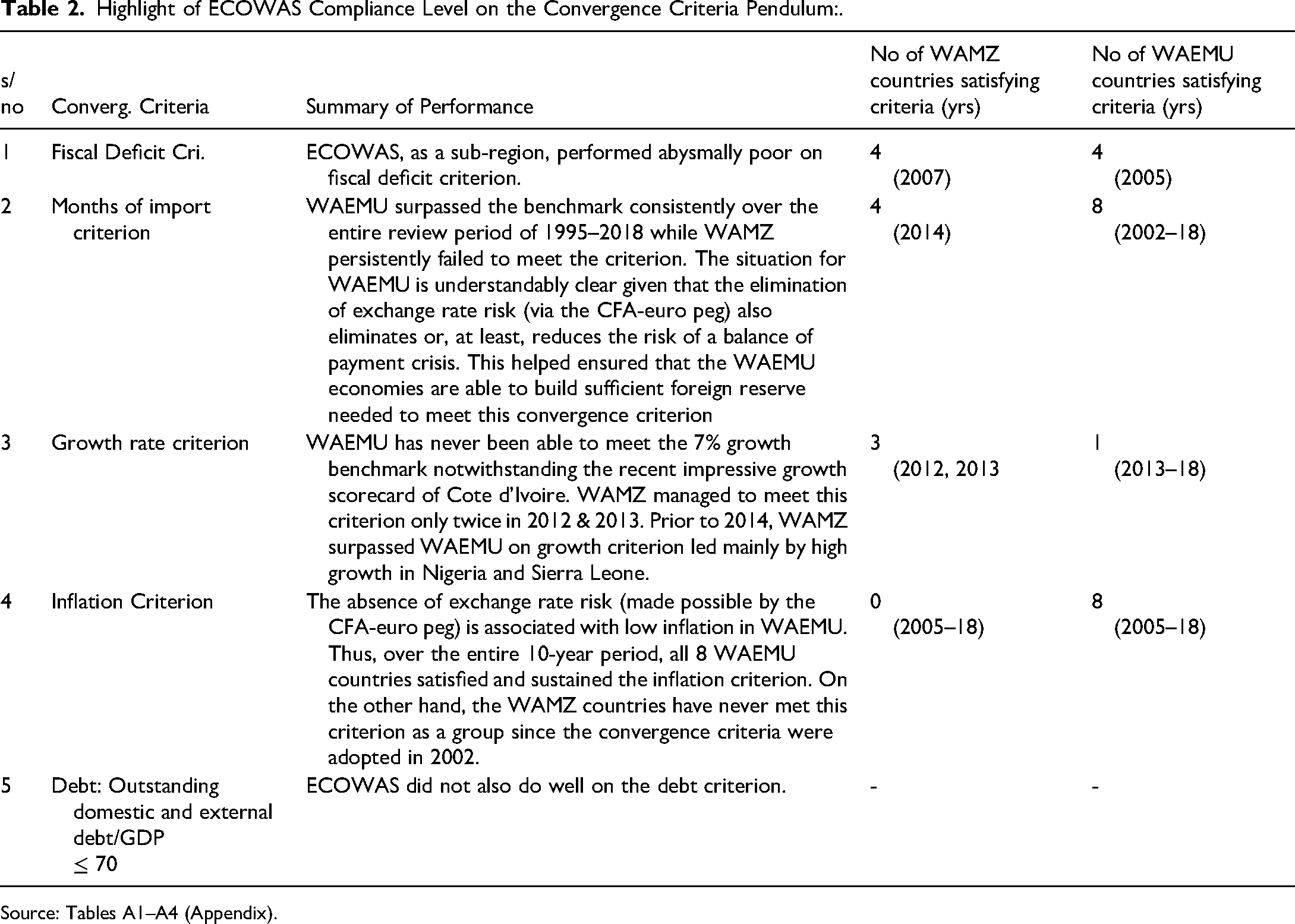
Source: Tables A1–A4 (Appendix).

Those with dissenting views regarding the structure of monetary union arrangement in ECOWAS are quick to point to two major related issues. First, they contend that the convergence criteria could constrain the use of fiscal policy in the future monetary union precisely when the countries in the region need it the most, having lost their autonomous monetary policy (see e.g., Alby, 2018; Allsopp & Vine, 1996; Gali et al., 2003 for EMU experience).⁴ If this presumption is true, it simply means that rule-based fiscal policy targets such as the ones imposed by convergence criteria may potentially constrain the ability of ECOWAS countries to implement countercyclical fiscal policies upon the launch of a common currency in the region. The problem appears even more compounded by the fact that fiscal rules do not take into account cyclical conditions in the economy.

A second and related argument often made, as Gali et al. (2003) demonstrate, is that recession can be deepened by efforts to raise taxes and cut spending when cyclical downturns increase deficits toward the benchmarks set by the convergence criteria. Therefore, the need to balance the budget against the constraints imposed by the convergence rules over the business cycle may imply a pro-cyclical fiscal policy that could rather amplify economic fluctuations in a future monetary union of WAMZ and WAEMU economies. In this regard, a common notion that is generally held is that monetary unions in-the-making must be guided by the lessons of the EMU – such as the financial and sovereign debt crisis in Greece, Spain, Portugal, Ireland and Italy; the failure of the Stability and Growth Pact (SGP); and, more recently, the exit of Britain from European Union, the so-called Brexit⁵ (Sissoho et al., 2015). While these arguments may have become part of received wisdom, there is very scanty empirical evidence to support them.

This paper seeks to investigate the extent to which constraints associated with the convergence criteria may have impacted the ability of governments of ECOWAS countries to conduct counter-cyclical fiscal policy and to understand how member countries have used discretionary fiscal policy as a stabilizing tool over the past two decades. The study of how national governments in the ECOWAS sub-region have used discretionary fiscal policy as a stabilization tool is unique for several reasons. First, as properly designed and implemented fiscal rules could help strengthen the credibility of government’s commitment to macroeconomic convergence and foster sound countercyclical fiscal policy, understanding the role of discretionary policy in economic stabilization becomes compelling and apt for countries in the sub-region.

Second, in view of the inability of most WAMZ and WAEMU countries to satisfy and sustain the convergence criteria, understanding how the convergence-related benchmarks have impacted their capacity to pursue counter-cyclical policy will inform policy for countries in the ECOWAS sub-region and supply lessons for the future monetary union of WAEMU and WAMZ. Third, although there is some knowledge of how the constraints imposed by fiscal rules could impact the capacity and/or motivation of countries to implement active counter-cyclical fiscal policies (see e.g., Allsopp & Vine, 1996; Gali et al., 2003 for the EMU countries, and Chang et al., 2002 for Asia countries), there is scarcely any robust empirical evidence on this for ECOWAS countries.

In particular, there is little or no knowledge of how the convergence related benchmarks have impacted the ability of national economies in the ECOWAS sub-region to maintain and increase public investments and raise capital stock. Little is also known of how convergence related constraints on fiscal policy may have impacted the ability of countries in the zone to use fiscal policy for economic stabilization. Therefore, as any convergence-induced restriction on counter-cyclical fiscal policymaking could have a long-run effect on the countries growth potentials, it becomes important to thoroughly investigate whether and how the convergence benchmarks may have made fiscal policy pro-cyclical.

We use insights from stylized facts and carefully specified regression estimation equations to investigate the discretionary fiscal policy reaction to output gap, investment, and lagged discretionary deficit, and a debt stabilization motive, among other drivers of cyclical condition. In particular, we estimate a Fixed Effect model and account for structural break (in 2002) in the full year specification using and interactive output-gap dummy for 14 ECOWAS countries over the period 1995 to 2018. Data retrieved from IMF fiscal monitor on debt and fiscal balance are used in the analysis, while data on other macroeconomic indicators are collected from the World Development Indicators (WDI) and UNCTAD. The main results of the study shows that, against the presumption of the dissenting viewpoint, fiscal policy has rather become counter-cyclical in ECOWAS following the introduction of the convergence criteria.

Overall, we find broad support indicating that the convergence criteria have not made fiscal policy less countercyclical in the convergence era in ECOWAS. There is evidence of a switch from pro-cyclical fiscal policymaking in the pre-convergence era (1995–2002) to counter-cyclical fiscal policymaking in the convergence era (2003–2018). Discretionary fiscal policy is also found to respond negatively to initial debt and initial deficit suggesting that fiscal policymaking in the pre-convergence era could be one that takes clue from initial debt and initial deficit rather than one that focuses explicitly on achieving a rule-based fiscal benchmark/target such as the one set by the convergence criteria.

To be clear, a statement of what our result implies - or do not imply - is in order. We make no claim that the countries that utilize discretionary fiscal policy do so because of the constraints imposed by the convergence criteria. What our result clearly shows is that the constraints associated with the convergence criteria have not made fiscal policy pro-cyclical. Instead, we found evidence to the contrary, namely; that fiscal policy has been more counter-cyclical in the convergence period in ECOWAS. The baseline result generally survives well under different robustness checks. The coefficient of output gap remains countercyclical both for the convergence era (2003–2018) specification and the full year (1995–2018) model that accounts for structural break. One key implication of our result for policy is that national governments should consider more flexibility in fiscal policymaking - against the constraints imposed by the convergence rules - through discretionary fiscal policy that balances the budget over the business cycle, rather than annually. There is also a clear need for the ECOWAS convergence council to adopt ‘discretionary fiscal deficit’ which represents real effort made to correct a excess deficit in their assessment of member countries’ compliance with the convergence benchmarks.

Our paper is related, in a broad sense, to three different strands of literature: the large literature on discretionary fiscal policy and automatic stabilizer (see Alagidede & Tweneboah, 2015; Arai, 2011; Afonso & Rault, 2010; Prohl & Westerlund, 2009; Alesina et al., 2008; Auerbach, 2002; Lane, 2002; Afonso, 2000; Hercowitz & Strawczynski, 1999; and Areaza et al., 1999; the literature on macroeconomic convergence and the political (and economic) business cycle (see Sissoho et al., 2015; Tarawalie et al., 2013); and more closely, the literature investigating the discretionary (and cyclical) response of fiscal policy to drivers of cyclical conditions such as GDP growth, output, or some variants of its measures – such as output gap (see Gali et al., 2003; Chang et al., 2002; Wyplosz, 2002; Fatas & Mihov, 2002; Martinez-Mongay, 2002; Lee and Sung (2007) Afonso & Furceri, 2010). Our study is an improvement and extension to some of these studies in a few dimensions. First, by following the standard IMF (same as OECD) procedure to decompose total fiscal deficit into its discretionary and automatic components, we depart from many past contributions that utilize cyclically unadjusted deficit (total fiscal deficit). Thus we able to adequately capture and identify in a precise and more comprehensive manner the discretionary reactions of fiscal policy to economic conditions (from the cyclical or automatic responses) in our estimated empirical fiscal policy rule.

Second, by also incorporating debt (and not merely expressing discretionary deficit as a function of the output gap or lagged discretionary deficit as in Afonso & Rault, 2010), we are better able to account for a debt stabilization motive of the fiscal authority. Finally, our methodology goes a step further by accounting for a structural break in the Fixed Effect model in view of the introduction of convergence criteria in 2002. By incorporating an interactive dummy for a structural break, we are able to avert specification bias by controlling for the differences in slope and in the intercept of our regression model in the pre-convergence and convergence periods in ECOWAS.

The balance of the paper is as follows. In Section 2, we present stylized facts on macroeconomic fundamentals and the scorecard of ECOWAS countries on the convergence scoreboard. This section also discusses the political economy of macroeconomic convergence with a view to unearthing why there is poor compliance with the convergence criteria among ECOWAS. Section 3 deals with an eclectic review of related literature. Section 4 lays out the empirical strategy and data description while section 5 concludes the study with some policy insights.

Stylized Facts on ECOWAS & the Political Economy of Poor Convergence

This section briefly interrogates the data, descriptively, on monetary union convergence with a specific focus on fiscal policy cyclicality (see section 2.2). We leave the more detailed descriptive Tables of the convergence benchmarks in the appendix in order to continue to maintain the focus of the paper which is on the procyclicality or countercyclicality of fiscal policy. To better understand the contemporary ECOWAS convergence experience, we set out with the discussion of the ECOWAS Monetary Cooperation Program (EMCP) which provides the needed legal framework for the adoption of the convergence criteria and for the establishment of convergence council that monitors compliance.

Macroeconomic Convergence Status in ECOWAS (2004–2018)⁶

Since ECOWAS was formed in 1975, its major vision has remained to create a regional economic space having a single market and common currency (the proposed eco) that would accelerate the pace of her economic development (Qureshi & Tsangarides, 2006; Saka et al., 2015; and Jebuni et al., 1999). In this regard, ECOWAS in July 1987 adopted the ECOWAS Monetary Cooperation Programme (EMCP) with the specific objectives of: (i) strengthening and improving sub-regional payments systems under the West African Clearing House (now West African Monetary Agency - WAMA) which is needed for the proper functioning of the single market; and (ii) establishing a single monetary zone, a common central bank and then a common currency (eco, now set for 2020).

The EMCP contained a set of macroeconomic convergence criteria that member countries were expected to observe prior to the emergence of the monetary union. The rationale for adopting the convergence criteria is to ensure convergence and synchronization of economic policies and fundamentals among prospective Member States so as to be able to manage the perceived challenges to the future monetary union of WAMZ and WAEMU countries – including differences in performance of macroeconomic fundamentals and disparity in shock affecting the economies. Table 1 shows the sets of primary and secondary convergence criteria for the ECOWAS sub-region, the WAMZ and the WAEMU areas.

Table 1.

Convergence Criteria in ECOWAS, WAMZ, and WAEMU.

ECOWAS
Primary Criteria	Secondary Criteria
1. Average annual inflation rate ≤ 5%	1. Non-accumulation of domestic and external arrears and settlement of all outstanding arrears
2. Overall fiscal deficit including grants/GDP ratio ≤ 3%	2. Tax revenue/GDP ratio ≥20%
3. Central Bank financing of the budget deficit ≤ 10% of previous year’s tax revenue	3. Wage bill/tax revenue ≤35%
4. Gross reserves ≥6 months of import cover.	4. Internally funded public investment/tax revenue ≥ 20%
	5. Positive real interest rate
	6. Real GDP growth rate ≥ 7%
WAMZ
Primary Criteria	Secondary Criteria
1. Average annual inflation rate ≤ 10%	1. Non-accumulation of domestic and external arrears and settlement of all outstanding arrears
2. Overall fiscal deficit including grants/GDP ratio ≤3% [or overall fiscal deficit excluding grants/GDP ratio (or budget deficit excluding grant) ≤4%]	2. Tax revenue/GDP ratio ≥ 20%
3. Central Bank financing of the budget deficit < 10% of previous year’s tax revenue	3. Wage bill/tax revenue ≤ 35%
4. Gross reserves > 3 months of import cover.	4. Internally funded public investment/tax revenue ≥ 20%
	5. Positive real interest rate
	6. Real GDP growth rate ≥7%
WAEMU
Primary Criteria	Secondary Criteria
1. Average annual inflation rate ≤ 3%	1. Payment arrears: non-accumulation of payment arrears in the management of the current period.
2. Basic fiscal balance/nominal GDP ratio ≥ 0	2. Tax revenue/GDP ratio ≥ 17%
3. Outstanding domestic and external debt/GDP ≤ 70	3. Wage bill/tax revenue ≤35%
	4. Internally funded public investment/tax revenue > 20%

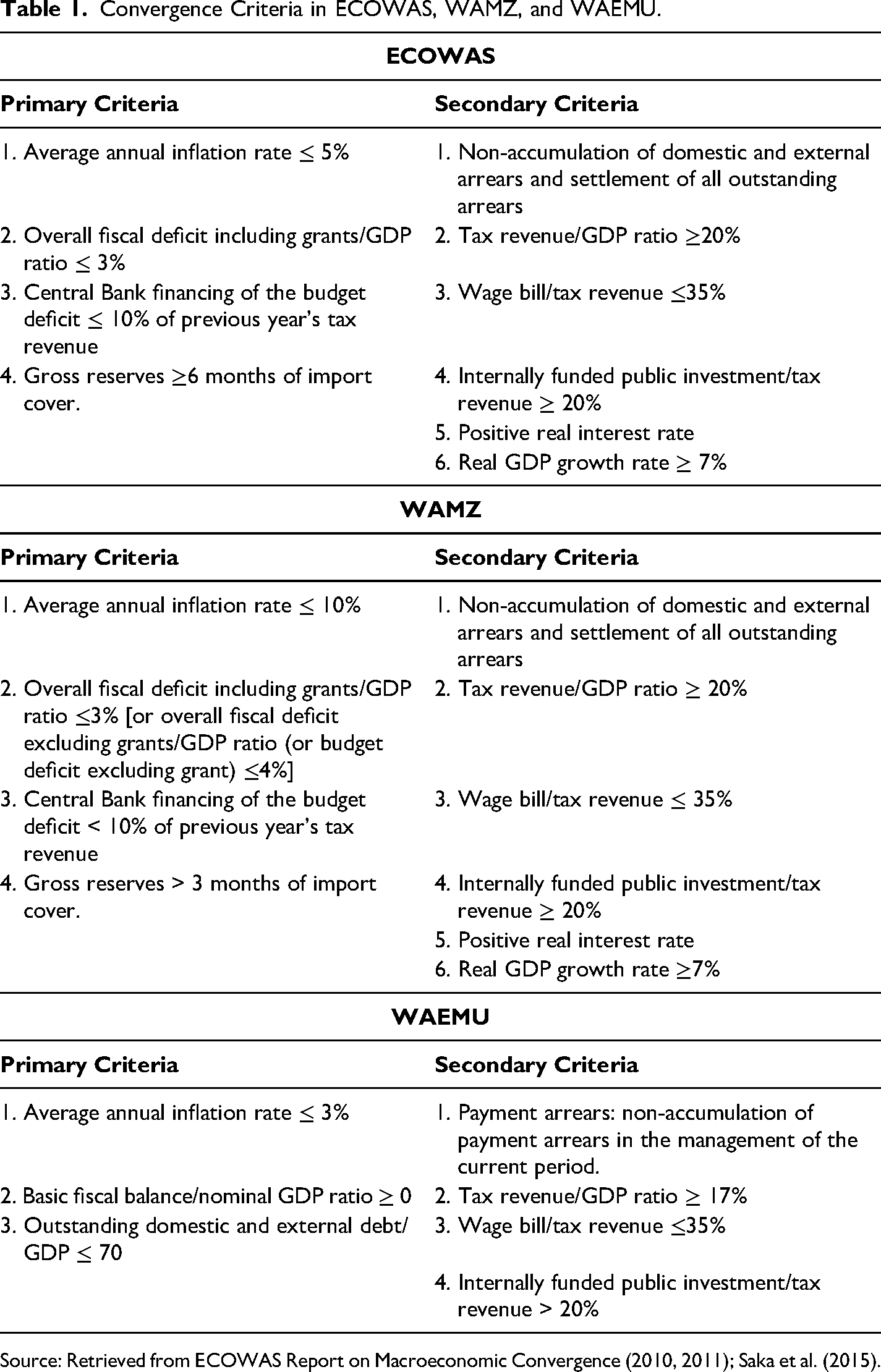
Source: Retrieved from ECOWAS Report on Macroeconomic Convergence (2010, 2011); Saka et al. (2015).

Thus, in 2000 the six WAMZ Member States adopted the two sets of convergence criteria (primary and secondary) that are meant to ensure convergence in critical macroeconomic variables in the economies.⁷ The WAEMU countries are also expected to observe these sets of critical convergence criteria – being a signatory to the ECOWAS Monetary Cooperation Programme (EMCP).

In the WAMZ area, however, a perceptive stylized review of the multilateral surveillance operations conducted by WAMI to assess WAMZ Member States’ compliance with the convergence criteria reveals that most of the countries in the zone find it difficult to satisfy and sustain their performance on the convergence scale. This has led to the postponement of the launch of the common currency for over 4 times from the initial date of 2003 to 2005, and then to 2009, 2015, and now 2020. Zooming in on the compliance profile of the WAEMU countries, we also see just a similar disappointing narrative.

Table 2 provides a synopsis of the ‘summary-statistics’ of ECOWAS (WAMZ & WAEMU) compliance level with the convergence criteria reported in Tables A1–A6 in the appendix. In concrete terms, the compliance level of each convergence criteria – namely those of the benchmarks on the deficit, months of import, growth rate, inflation, and debt is reported in Tables A1 through A6, respectively.

Markedly, there isn’t any single year in which at least more than half of either the six WAMZ or eight WAEMU countries are able to satisfy deficit criterion (see Table A1). WAMZ as a group has persistently overshot the ‘fiscal deficit ≤ 4%’ benchmark over the past one and half-decades. In terms of the number of countries satisfying this criterion, the best-performing year for WAMZ is 2007 when a maximum of 4 countries \satisfied this criterion. The WAEMU countries even appear to have performed worse than the WAMZ countries on this criterion. Over the preceding 4 years (2015–2018) no single WAEMU country met the fiscal deficit criteria. Thus, considering the average fiscal balance for the ECOWAS region as a whole (Figure 1), we see a situation where the region has managed to maintain a fiscal balance between 2004 up to 2008 and has thereafter consistently operated fiscal deficit particularly between 2009 and 2018.

Figure 1.

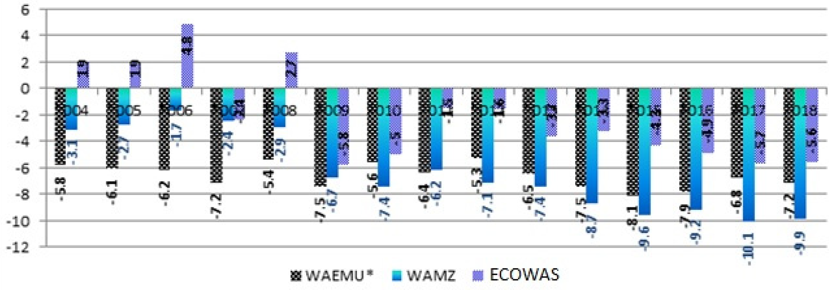
Fiscal balance, excluding grants (% GDP) in the ECOWAS, WAMZ and WAEMU areas (2004–2018). Source: WDI (2019). Note: Regional balance is based on the average balance for each region.

In terms of the month of import criteria, the WAEMU has done impressively well by continually surpassing the ‘external reserve > 3 months of import’ benchmark but this is not too surprising given that as a member of the CFA zone, the risk of a balance of payments crisis is eliminated de facto, as long as the guarantee by the French Treasury of unlimited convertibility of the (African Financial Community) CFA Franc is ensured. According to Seck (2013) and as recently alluded in Alby (2018), this is a big advantage for these countries that are basically exporters of primary commodities. Considering the case of Ghana and Cote d’Ivoire, for instance, that have a similar economic structure as exporters of primary commodity (cocoa), this scenario is succinctly demonstrated in the spectacular deterioration of Ghana’s macro-financial situation during a period when Cote d’Ivoire remained resilient even in her post-electoral crisis in late 2010 and early 2011.⁸ Looking at WAMZ countries, Nigeria has particularly benefited from the prolonged favourable crude oil prices with a peak of financing over 12 months of imports in 2008. On the flip side, Guinea’s poor performance in this criterion, especially in recent times, has particularly been driven by the prolonged macroeconomic weakness of the economy.

Interestingly, a careful stylized account of the regional growth performance could provide important insights into the convergence assessment. GDP growth rate in the WAMZ area consistently surpassed those of the WAEMU area in the period preceding the year 2014, i.e., between 2006 to 2013 (Table A3). And this was led mainly by the growth rate in Liberia, Nigeria and Sierra Leone during the 8-year period. However, a reversal started in 2014 when the average GDP growth rate in WAEMU - led mainly by the growth rate of Cote d’Ivoire - began to surpass those of WAMZ. Over the past half decades (2014–2018) WAEMU’s GDP growth rate has continually exceeded the average GDP growth rate in the WAMZ area. The highest regional GDP growth rate was recorded in 2013 at 8.5%. More recently, the WAMZ region has witnessed rather unimpressive growth performances as the growth rate for the zone dipped to −1.0% (led mainly by the slowdowns in Sierra Leone) and 3.2% in 2015 and 2016 respectively from an average of 8.0% and 8.5% in 2012 and 2013 respectively. As of 2018 and 2017, the WAMZ growth rate stood at 4.2% and 4.6% respectively compared to the higher GDP growth rate of 6.1% and 5.7% over the same periods in the WAEMU area.

Taking the country-specific experiences into account, it is evident that the Member States have performed poorly over the preceding half-decade. This has generally been attributed to the lingering effect of declining commodity prices. The real GDP growth rate moderated in The Gambia to 2.2% in 2016 from 4.3% in 2015 and 4.8%in 2013. This had resulted from adverse weather conditions, the decline in foreign exchange reserves resulting from fall in export, and the uncertainty that surrounded the 2016 general election in The Gambia (see WAMI Annual Report 2015, 2016). Similarly, the growth rate was sluggish in Ghana over the period 2014–2016 except in 2017 and 2018 when growth in Ghana surpassed those in all other WAMZ economies. This is mainly on account of an increase in the production of gold and oil and gas in the recent history of Ghana. Over the past four years, Nigeria’s growth rate has been unimpressive as the economy witnessed a persistent decline in growth, from 6.3% in 2015 to a negative growth rate of −1.6% in 2016 when the country plunged into recession. Nigeria’s 2016 economic recession was orchestrated by plummeting price of crude oil (the major source of foreign exchange) which resulted in a drastic drain of the country’s foreign exchange reserve. Modest recoveries have been made with Nigeria posting a growth rate of 0.8% and 1.9% in 2017 and 2018 respectively.

Overall, the recent modest growth rate in the WAEMU area has been led mainly by Cote d’Ivoire whose growth rate has consistently surpassed the threshold ‘real GDP ≥ 7%’ for a period of 7 consecutive years, 2012–2018 (Table A3). Notwithstanding Cote d’Ivoire’s consistent impressive real growth scorecard over the six-year period (2013–18), the ECOWAS region’s growth scorecard has been abysmal.

The situation for the inflation criterion is not different. Due to the absence of exchange rate risk implied by the CFA franc’s peg to the euro and the resultant low inflation associated with such stability in the exchange rate, the inflation criterion was assigned different benchmarks for the WAEMU and WAMZ area particularly as countries in the later zone generally operates free float exchange rate systems (annual inflation ≤10% for WAMZ and ≤3% for WAEMU). While the WAEMU region has been able to satisfy the WAEMU’s inflation criterion over the past decade (2009–2018) WAMZ area has never met WAMZ’s inflation criterion as a group (Tables 2 and A4).

The Cyclicality of Output Gap and Dynamics of Debt and Deficit (1995–2018)

This sub-section focuses on the basic matter of deficit and debt dynamics that undermines fiscal policy procyclicality/countercyclicality and, therefore, also drives the cyclicality of output gap (Figure 3). A careful stylized characterization of the total fiscal deficit and debt profile of countries in the region reveals unique structural patterns, including (i) large and growing trend of fiscal deficit; (ii) a large and looming total external debt stock, current $US (reflecting the accumulation of yearly deficits) as well rising private debt (% GDP). This is notwithstanding the decline and apparent convergence in debt ratios. Markedly, given the looming debt stock – external, domestic and private ($US) – the apparent decline and convergence in both the total central government debt (% GDP) and external debt (% GNI) in ECOWAS are no very innocuous. In fact, it calls to question the appropriateness of the use of debt/GDP ratio for debt sustainability analysis especially because debt is not paid back with GDP but with revenue. Evidently, the observed swings of output gap (±5% band) appear to have tended to undermine the modest growth performance of the mid-2000s and early 2010s previously reported.

Figure 2.

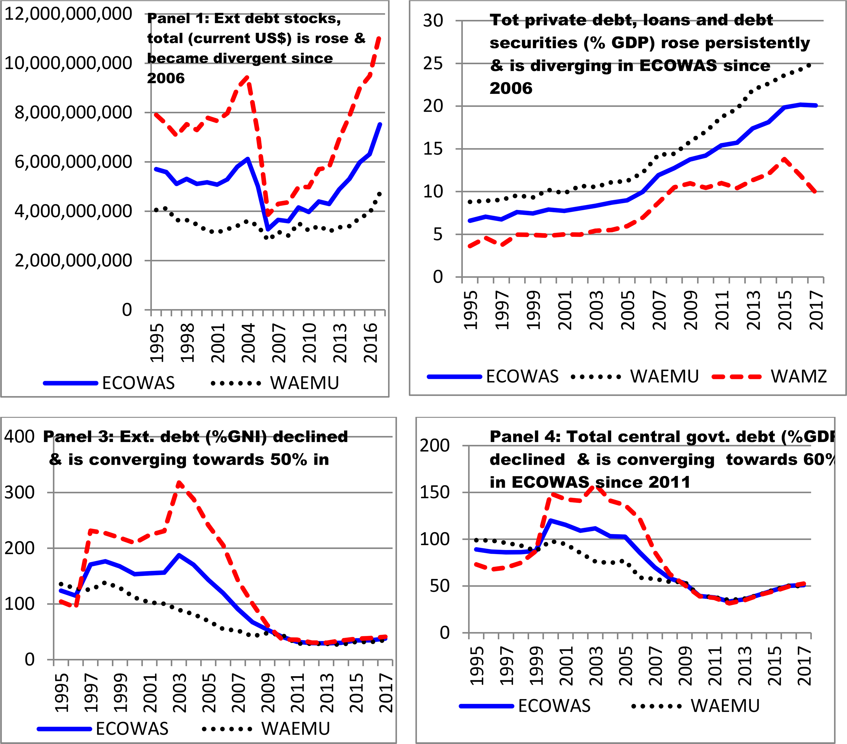
Trend of public debt (stock, ratio) & private debt in ECOWAS 1995–2017. Source: WDI (2019)-external debt stock (% GNI) & total debt Stock (Current $US); IMF (2019) - total central govt. debt (%GDP) & total private debt, loans and debt securities (% GDP).

Figure 3.

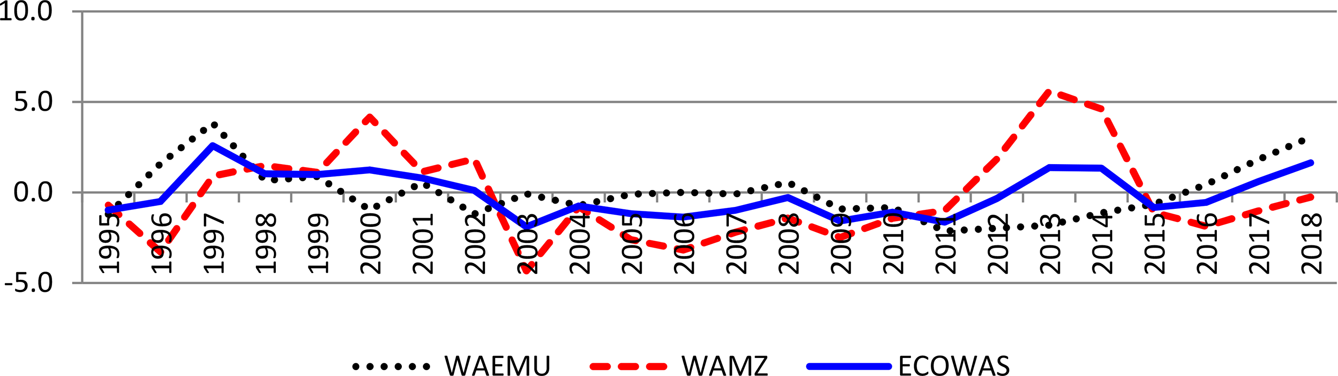
Trend of output Gap in ECOWAS, WAEMU, and WAMZ. Source: WDI (2018).

We set out with a more specific analysis of debt as this represents an accumulation of yearly deficits. Thereafter, the decomposition of the total fiscal deficit into the cyclical and potential components is discussed.

Figure 2 - comprising of 4 panels (1 to 4) – shows the evolution of public debt, namely: total external debt stocks (current US$), external debt (% GNI) and total central government debt (% GDP) in panels 1, 3 and 4 respectively. It also shows total private debt, loans and debt securities (% GDP) in panel 2. The general picture that emerges from Figure 2 is that total debt stock (in monetary terms) is huge and rose persistently since 2006, and this has been closed mimicked by the bullish trend of private debt since 2006. This is notwithstanding the decline in the central government and external debt ratios. Arguably and as has been noted, the apparent decline and convergence in debt ratio do not reduce the critically of the rising debt profile in ECOWAS because the debt stock (measured in monetary terms, current US$) clearly rose. This is important because debts are repaid with revenue and not with GDP. And so, the use of debt/GDP ratio for debt sustainability assessment might soon begin to lose the fancy of intrepid researchers. Moreover, the need to also analyze private debt stock is gaining increasing attention because as Mbaye et al. (2018) document in their recent IMF paper – “Bailing Out the People? When Private Debt Becomes Public” – excessive private debt could systematically turn into higher public debt via a debt migration process that operates through growth rather than explicit bailouts.

Because debt represents the accumulation of yearly deficit and since deficit reflects a major driver of fiscal policy cyclicality and therefore business cycle, the final thing we examine in this sub-section is the dynamics of output gap over the sample period (1995–2018). This is important because the trust of any stabilization fiscal policy is to close the GDP gap as much as possible, i.e., to avoid wide swings in output. From a fiscal policy perspective, an assessment of the output gap is also important in determining the extent to which developments in public finances such as fiscal deficits are cyclical or discretional (Darby & McIntyre, 2018, p. 20).

Notably, the GDP gap and output gap are two closely related concepts but a subtle difference exists. A distinction between the two is in order. Statistically, GDP gap is equal to actual GDP less potential GDP. On the other hand, output gap is simply equal to GDP gap (cyclical GDP) expressed in percentage of potential GDP (see Danmarks National Bank Monetary Review 4^th Quarter, 2015). In fact, what the HP filter does is to calculate the potential GDP from the actual GDP and report the difference between them as the cyclical GDP (see Central Bank of Iceland Monetary Bulletin, 2005; Hodrick & Edward, 1997). In the estimation of our empirical fiscal policy reaction function (eq.5 and 6), we use, as the dependent variable, the discretionary deficit (DISC) computed using the IMF approach as specified by equation 3.

Thus, a mathematical formalization of these relationships can be presented thus,

G D P g a p = r e a l G D P - p o t e n t i a l G D P

(1)

where

G D P g a p \equiv c y c l i c a l G D P

O U T P U T g a p = (\frac{c y c l i c a l G D P}{p o t e n t i a l G D P}) \times \frac{100}{1}

(2)

An explanation of equations 1 and 2 is in order. Throughout this paper, we employ the HP filter in calculating the cyclical and potential components of only two variables, namely: the real GDP and the total fiscal deficit. Regarding the real GDP, the HP filter calculates the potential GDP and the cyclical GDP from the real GDP data. Equation 1 simply shows that GDP gap is real GDP minus Potential GDP. On the other hand, equation 2 indicates that output gap is calculated as the ratio of cyclical GDP to potential GDP (expressed as a percentage). Markedly, the output gap (equation 2) is based on the authors’ calculation using cyclical GDP and potential GDP data obtained by the HP filter. In turn, the output gap data is combined with real GDP and total fiscal deficit data to calculate discretionary fiscal deficit using the IMF formal approach for doing this (see Fedelino et al., 2009; Gali et al., 2003; Mourre et al., 2013; see eq.4). Both the discretionary deficit and output gap are used in the estimation of the empirical fiscal policy reaction function specified as equation 6 in the sequel.

Markedly, an output gap that is positive and rising indicates that the economy is overheating, i.e., the actual GDP is rising beyond the potential GDP and that contractionary fiscal policy is needed to bring actual real GDP back to equilibrium. On the other hand, an emerging negative output gap implies that there is spare capacity, or slack, in the economy due to deficient demand. In this case, the real GDP lags behind its potential value and an expansionary fiscal policy are needed to boost economic activity and restore equilibrium.

Figure 3 shows that the output gap has hovered within ± 5% band over the sample period. The fundamental questions here are as follows; (i) how has discretionary fiscal policy been able to restore the equilibrium (achieve output stabilization)? and (ii) how have the constraints on ‘fiscal’ policy associated with the convergence criteria impacted the ability of ECOWAS economies to restore equilibrium (stabilize the economy) using active countercyclical policies? We leave the precise answers to the more robust estimation technique, the fixed-effect model.

Dynamics of Cyclical, Potential and Total Fiscal Deficit in ECOWAS (1995–2018)

Because theory without facts could put one in a blind alley, we let the data speak. In this sub-section, therefore, we descriptively interrogate the data on fiscal deficit by closely looking at the trend of total fiscal deficit – operationally defined as the amount by which total general government spending exceeds total general government revenue - in 14 ECOWAS economies for which consistent data are available. Figure 4 shows the evolution of total fiscal deficit, cyclical deficit and potential deficit in the 14 ECOWAS countries; namely 6 WAMZ countries (Gambia, Ghana, Guinea, Liberia, Nigeria, Sierra Leone) and 8 WAEMU countries (Cote d’Ivoire, Benin Republic, Burkina Fasso, Guinea-Bissau, Senegal, Mali, Niger, Togo) between 1995 −2018.

Figure 4.

Trend of total fiscal deficit, cyclical deficit & potential deficit in ECOWAS (1995–2018). Source: IMF’s WEO Database (2018). While the cyclical component of the total fiscal deficit is scaled on the left-vertical axis, the potential component and the actual fiscal deficit are scaled on the right-vertical axis. Note: total fiscal deficit is measured in billions of Local Currency Units (LCU). Key: The graph is based on Hodrick-Prescott Filter at Lambda, 100 (see the section on the methodology for rationalization of choice of λ = 100). Due to the dearth of consistent budget data (over the entire sample period) for most countries in our sample, we use the total fiscal deficit (rather than budget deficit). The fiscal deficit (general government) is defined as the fiscal position of government after accounting for capital expenditure. Operationally, it is obtained as general government’s total expenditure less general government’s total revenue. While total fiscal balance, is statistically defined as the net lending of the general government (revenue less expenditure), the total fiscal deficit is defined as the excess of expenditure over revenue (expenditure less revenue). In this sense, if the sign of the total fiscal deficit is negative, it is called total fiscal balance which implies net lending of the general government. As Mourre et al. (2013) note, government balance according to the EDP (excessive deficit procedure) definition is the net lending (surplus) / net borrowing (deficit) of the general government. The concept of total fiscal deficit as clearly defined here differs from the concept of ‘primary deficit’ which is simply total fiscal deficit less interest payment.

While the cyclical component of the total fiscal deficit is scaled on the left-vertical axis, the potential component and the actual fiscal deficit are scaled on the right-vertical axis.

Figure 4 comprises of 14 panels (A to N) for the 14 ECOWAS countries in our sample. Each panel plots the trend of total fiscal deficit and its corresponding cyclical and potential components retrieved via Hodrick-Prescott’s filtering approach. The green lines with box-annotations indicate the cyclical component of the total deficit of the respective economies. On the other hand, the blue solid line and the red line that trails them (annotated with a star) depict the total fiscal deficit and the potential fiscal deficits, respectively. Expectedly, potential deficit trails the total deficits across the countries. By simply eyeballing Figure 4, it can be seen that despite the adoption of convergence criteria since 2002, the total deficit has persistently increased in all 14 ECOWAS countries. The rate of increase appears to be high irrespective of the relative size of the economies. This clearly alludes to the preponderance of negative fiscal balance earlier reported in Figure 1 (and Table A1) and also explains the large and rising debt stock (in $US) shown in Figure 2. Expectedly, this is so because debt simply represents the accumulation of yearly deficits.

Calculating Discretionary Deficit – IMF (and OECD) Approach

As noted, discretionary deficit is calculated from total fiscal deficit, output gap and real GDP data using equations 3. As in Gali et al. (2003) and Mourre et al. (2013), our empirical fiscal policy reaction function relies on the discretionary deficit as the dependent variable. The terms discretionary deficit simply refer to the component of the total fiscal deficit that is due to the conscious policy decision or action of the government (or policymaker) rather than automatic changes in economic activity.⁹ The concept of discretionary fiscal policy is very important for use in the analysis of fiscal policy in the following areas: (i) as Mourre et al. (2013, p. 7) for instance note, it is useful in assessing fiscal sustainability issues.¹⁰ An example is its application in comparing the discretionary deficit against a pre-determined debt-stabilizing discretionary deficit; (ii) it is also useful for designing adequate fiscal consolidation policies that can help a region like Africa avert the looming debt crisis or, at least, grow with debt. For instance, following the 2005 and 2011 reforms of the Stability and Growth Pact (SGP) in the EU, discretionary deficit has become a key indicator for assessment of country-specific medium-term fiscal objectives under the “preventive arm” and the assessment of “effective action” in the context of excessive deficit procedure (the “corrective arm). The discretionary deficit is recommended for use by the surveillance council in ECOWAS in addition to the fiscal balance (% GDP) that is currently in use because discretionary deficit provides a better framework. In fact, it actually represents effort achieved to correct excessive total deficit (see Mourre et al., 2013 for a discussion).

The calculation of discretionary deficit from total fiscal deficit is well documented in the literature (see e.g., Fedelino et al., 2009; Gali et al., 2003; Mourre et al., 2013). For instance, as Gali et al. (2003, p. 543) note, the removal of the cyclical component of deficit from total fiscal deficit aims at measuring the fiscal stance intentionally chosen by policymakers rather than the result of uncontrolled economic fluctuations. The same authors isolated the discretionary deficit (for a number of EMU countries) from the total fiscal deficit and used the discretionary component in the estimation of a set of fiscal policy reaction functions.

As in Mourre et al. (2013), our study makes use of a formal approach (used by the IMF, OECD, and EMU) in calculating discretionary deficit. In particular, we make use of the approach that is based on ‘sensitivity’, rather than ‘semi-elasticity’ measure of budget or fiscal parameter. This approach is preferred to the “semi-elasticity’ approach because as Mourre et al. (2013) demonstrates, the latter requires over six different measures of revenue and expenditure elasticity, i.e., unemployment related elasticity, that are not readily available for developing countries.

Following the approach used by the IMF and OECD (see e.g, Fedelino et al., 2009; Gali et al., 2003; Mourre et al., 2013; Ter-Minassian, 2010), discretionary deficit (DISC) is computed using the following formula:

D I S C = \frac{f D e f}{G D P} \times [O G (\frac{Δ f D e f}{Δ G D P})]

(3)

Where: DISC represents discretionary deficit, which is defined as the component of the total fiscal deficit due to the deliberate policy choice of the government);

f D e f

represents the total fiscal deficit which is defined as the general government total expenditure less general government total revenue. OG represents for output gap which is defined by equation 2;

(\frac{Δ f D e f}{Δ G D P})

represents a measure of fiscal or budget parameter defined as the marginal rate of change of deficit with respect to change in the level of real GDP, and ‘Δ’ stands for a first difference operator (see Table A6 for data sources and variable definitions).

Equation 3 simply shows that discretionary deficit can easily be calculated once we have data on three core variables, namely: output gap, total fiscal deficit, and real GDP. We have earlier noted that the output gap (equation 2) is based on the authors’ calculation using data on potential and cyclical GDP retrieved via the HP filter.

Why are ECOWAS Countries not Meeting the CC-A Political Economy Perspective?

As noted in the opening paragraph of section 2, the ECOWAS Monetary Cooperation Programme, EMCP (adopted through Decision A/DEC.2/7/87 in 1987) contains a set of macroeconomic convergence criteria which member countries were expected to observe prior to the emergence of the monetary union (ECOWAS Commission Report, 2010). In furtherance to this, the ECOWAS macroeconomic convergence Criteria was adopted through Decision A/DEC.7/12/99; and to make the surveillance of macroeconomic policies operational, Decision A/DEC.17/12/01 establishing the mechanism for multilateral surveillance of economic and financial policies of ECOWAS Member States was also adopted by the Authority of Heads of State and Government. The rationale for adopting the convergence criteria is to ensure convergence and synchronization of economic policies and economic variables among potential Member States. This is, in fact, necessary to ensure that participating countries are better able to manage the perceived challenges to the future monetary union of WAMZ and WAEMU countries – including differences in performance of macroeconomic fundamentals and disparity in shock affecting the economies. In the WAMZ area, the convergence criteria were adopted in 2002 while WAEMU countries were expected to observe the convergence criteria since they were signatory to the EMCP.

Thus, recognizing that the convergence criteria are critical for the adoption of a common currency, recent effort appears to have extended well beyond their merit (see e.g Debrun et al., 2005; Gali et al., 2003; Saka et al., 2015; Seck, 2013). What now appears to be the major subject of discourse is; how best should macroeconomic convergence criteria be structured, and how best should compliance be enforced to enable participating countries to comply better? Stated differently, this is the question of why the level of compliance is poor. However, it is remarkable to note that while total convergence may not be necessary in practice (not all euro area countries satisfied the Maastricht criteria and the SGP before admission into the euro area and some like Britain got opt-out), the ECOWAS countries must be guided by the lesson of the EU – such as the financial and sovereign debt crisis in Greece, Spain, Portugal, Ireland and Italy; the failure of the Stability and Growth Pact (SGP); and, more recently, the attempt by Britain to exit the European Union. This notwithstanding, the fiscal rules/benchmarks as contained in the Convergence Criteria is massively critical to the successful formation of a monetary union in ECOWAS. This is because fiscal policy remains a national prerogative even after a monetary union is established (Saka et al., 2015). In the absence of a well-coordinated fiscal policy framework, undisciplined national fiscal policies with adverse spillover effects between member countries could conflict with a stability-oriented monetary policy and undermine the survival of the monetary union.

The debate, as noted, has instead focused more on the structure and design of the convergence criteria particularly in the following areas: (i) what constitutes the optimal fiscal policy rule or benchmark (e,g., what should be the optimal debt stabilizing fiscal deficit benchmark); and (ii) should the design of fiscal policy rule take business cycles into account. For instance, Wyplosz (2005) demonstrates that fiscal policy rules such as the ones imposed by the SGP (and the convergence criteria too) are bound to be counterproductive if they fail to recognize unforeseen circumstances such as cyclical downturns. This could occur when cyclical downturn increases deficit towards the limit set by the convergence criteria. Relating this to the experience of the EMU, the same author shows that the major reason for the failure of Stability and Growth Pact, SGP (which provides concrete content to the Maastricht Criteria and, more importantly, represents the most elaborate form of fiscal rule by including sanctions) is that it was designed to constrain deficit rather than eliminate it. The basic argument of this author is that rather than try to constrain deficit to the annual budget, effort should focus more on trying to eliminate it by allowing for more flexibility via the pursuit of (counter-cyclical) fiscal policy over the business cycle.

Narrowing down to the experience of ECOWAS countries and as Alby (2018:, p. 1) rightly notes, macroeconomic convergence criteria particularly in the WAEMU area have been set but are apparently not binding. For instance, unlike in the WAMZ area, there are no WAEMU-groomed institutions (aside from the ECOWAS surveillance mechanism that was adopted in 2001) to provide macroeconomic surveillance in order to ensure compliance with the convergence criteria. There is also no convergence council in the WAEMU area to the best of our knowledge. Even in the WAMZ area where such institutions have been established, compliance is also poor, perhaps, even poorer because the mere existence of a convergence council does not make the rules set by the convergence criteria binding. If the most comprehensive/ elaborate Convergence Criteria in the World – elaborate in the sense that they include sanctions – failed, how then would one expect a Convergence Criteria that are not binding because they failed to include sanctions to work? The issue of whether or not the sanctions are applied -which is the major reason for the failure of the SGP (Gali et al., 2003) - is a different matter.¹¹

Therefore, we document here that part of the salient reason for poor compliance with the convergence criteria in the ECOWAS sub-region is that the rules are not binding because they fail to include sanctions and this – as widely documented in the literature – have resulted mainly from lack of political commitment on the part of national governments apparently for erroneous fear of loss of political and economic sovereignty.

Other constraints that have been identified include (i) non-uniformity in the adoption of required macroeconomic framework and lack of policy coordination and harmonization between the Francophone West African countries with an established economic and Monetary Union (UEMOA) since 1994 and the Anglophone countries; (ii) different levels of development and shocks, distrust and suspicion among member countries; (iii) inadequate financial market and infrastructure, problem of regulating and supervising the financial market integration and how to conduct effective monetary and fiscal policies.

Given the above challenges militating compliance with the convergence criteria, what are the options for mitigating them to improve compliance in the ECOWAS region? These include: (i) renewed political commitment by national governments in ECOWAS to accelerate the implementation of different legal instruments adopted by the Community, such as the Protocol on free movement of persons and goods, right of residence and establishment, as well as the relevant provisions of the trade liberalization scheme (ii) enactment and strict implementation of the Fiscal Responsibility Act and the promotion of sound borrowing policies; (iii) application of discretionary deficit (DISC) by the convergence council for the assessment of the level of compliance with the convergence criteria to adequately capture action taken to correct excessive deficit in addition to the use of fiscal deficit/balance (%GDP) criterion; (iv) periodic and timely transmission of macroeconomic convergence reports by Member States to the ECOWAS Commission and in line with the framework adopted; and (v) continued efforts by the ECOWAS Commission to build the capacities. Finally, the introduction of sanctions – even if it is designed as an atomic bomb as with the Stability and Growth Pact (SGP) – should be a consideration.

But as Ekpo (2018), for instance, notes, there are some unsettled issues beyond the convergence criteria that ECOWAS countries must consider as the region moves towards monetary integration. These include the challenges associated with the process by which the Franco-phone countries would de-link from France, limited political will, huge infrastructure deficit, and fiscal imperatives.

Presently, the ECOWAS Commission has adopted a single-track (fast track) approach to a monetary union. The single-track approach does not consider the WAMZ or WAEMU as a bloc but focuses on any country within the ECOWAS that meets the convergence criteria, and therefore, becomes eligible to join the monetary union. In addition, any country that meets the convergence criteria at a point in time, the so-called point convergence, is also considered eligible to be admitted into the monetary union. The single-track approach to the monetary union was adopted in 2015. Its hallmark is, therefore, that the monetary union would commence with few countries that met the convergence criteria (e.g., on the basis of point-convergence) while other ECOWAS countries would be admitted into the union as they satisfy all or part of the convergence criteria (ECOWAS Convergence Report, 2016). However, and as in Ekpo (2018:, p. 2), whether the proposed year of 2020 for the establishment of the monetary union is feasible is still a matter of debate.

Review of Related Literature

Given the issue at hand, namely the role of fiscal policy in economic stabilization in the context of macroeconomic convergence benchmarks in ECOWAS, two major strands of literature are discernable. The first set focuses on macroeconomic convergence and the political (and economic) business cycle. The second strand of literature discusses the discretionary (structural) and cyclical (automatic) response of fiscal policy to drivers of cyclical conditions, especially GDP growth, output, or some variants of its measures – such as output gap.

Macroeconomic Convergence and Political Business Cycle Literature

A number of studies have investigated the effect of macroeconomic, political and institutional factors on the achievement of WAMZ convergence criteria. A good number of them are reported in various Occasional Papers of the Research Department of WAMI, and the AfDB working papers, among others.

For instance, Tarawalie et al. (2014) investigated the existence of a political business cycle in WAMZ countries and its effect on the attainment and sustenance of macroeconomic convergence criteria which is needed for the launch of a monetary union in the zone. Their study makes use of a hybrid of non-rational opportunistic and partisan Political Business Cycle (PBC) Model to analyze the implications of the PBC trend on fiscal outcomes, monetary aggregates and real sector variables. Their study revealed mixed results. In three of the six economies, namely; Nigeria, Gambia and Sierra Leone, the trend in PBC does not pose a serious challenge to compliance with convergence criteria. For instance, in spite of the existence of political business cycle (PBC) trend in Nigeria, fiscal deficit and inflationary spree were found to decline in election years and increase in non-election years. During election years in Nigeria, government spending tends to decline while revenue continues to rise, thus, leading to a declining deficit. The result for Ghana reveals significant PBC trends in both fiscal and monetary variables – signaling that Ghana could face a severe challenge in meeting the convergence criteria if the situation is not addressed. The result for Guinea mimics that of Ghana and suggests – according to the same authors – that ideological and opportunistic political behaviour could exert a deleterious effect on Guinea’s compliance with the primary convergence criteria.

Similarly, Tarawalie et al. (2013) used the Set-Theoretic Approach (STA) and Vector Autoregressive Model to analyze the degree of fiscal and monetary policy coordination among WAMZ economics and its implication for their attainment of convergence criteria. The VAR results indicate weak policy coordination in the zone that has contributed to non-compliance by the Member States with respect to inflation and fiscal deficit criteria.

In a related study, Sissoho et al. (2015) examined the implications of the recent EMU experiences, especially the Greek Debt Crisis for the macroeconomic convergence criteria in WAMZ and single currency project in ECOWAS. The study noted that two outstanding factors that led to the crisis are: (i) the statistical misreporting (or worse still falsification) of Greece debt and fiscal deficit information; and (ii) lack of effective fiscal policy supervision mechanism in EMU.

Discretionary and Automatic Stabilizer Literature

The literature on the cyclical sensitivity of fiscal policy, i.e., on the fiscal policy response to macroeconomic determinants of the cyclical condition, and of fiscal sustainability is biased towards the experience of major industrialized countries of Europe and America. Some of the recent works in this area include Alagidede and Tweneboah (2015); Arai (2011); Afonso and Rault (2010); Prohl and Westerlund (2009); Alesina et al. (2008); Gali et al. (2003); Chang et al. (2002); Wyplosz (2002); Auerbach (2002); Lane (2002); Fatas and Mihov (2002); Afonso (2000); Hercowitz and Strawczynski (1999); and Areaza et al. (1999); among others.

For instance, Gali et al. (2003) examined how the EMU governments have used discretionary fiscal policy as a stabilizing tool between 1978 and 2001 and whether the constraints associated with the Maastricht Treaty has constrained the EU governments’ ability to deploy counter-cyclical stabilization policy and to provide an adequate level of government services and public infrastructure. Their study, which covers 14 EU and 5 OECD countries, makes use of the Instrumental Variable (IV) regression technique with structural breaks at the year (1992) when MT was adopted. The study by Gali et al. (2003) show that contrary to the general belief, discretionary fiscal policy has been procyclical in pre-MT Germany and acyclical in the pre-MT United States, Italy, and United Kingdom. But in the MT-era, they found no evidence that discretionary fiscal policy was less counter-cyclical, and if anything – as their study shows – discretionary fiscal policy was more counter-cyclical in MT-era Europe following what appears to be a general trend that affects other industrialized countries as well.

Wyplosz (2002) conducted a study for four countries (Italy, Germany, UK, and the US) which is similar to that of Gali et al. (2003) for EMU countries. Although this study also accounted for a structural break in 1992, it made use of cyclically unadjusted deficit/GDP ratio. The result differs slightly from those of Gali et al. (2003). Wyplosz (2002) found that discretionary fiscal policy was rather countercyclical in the pre-MT United States and Italy and acyclical in MT-era Germany. The discrepancy in the result could be attributed to the cyclical component of deficit – which makes the fiscal policy response more countercyclical – but was unaccounted for in this study. In another related study, Auerbach (2002) found that the effect of changes in the growth rate of GDP and output gap on legislated changes in the budget surplus (analogous to the discretionary deficit) has been fairly more counter-cyclical in the US after 1992.

In their work, Fatas and Mihov (2002) regressed cyclically unadjusted primary deficit (total deficit less interest payment) on cyclical indicators (output gap, inflation and interest rate) and interpreted the residual from the estimated model as an indicator of the discretionary fiscal stance. Other works on OECD countries that are closely related to that of Fatas and Mihov (2002) include; Lane (2002), Areaza et al. (1999), and Hercowitz and Strawczynski (1999).

However, an evaluation of the literature in this area of the study reveals that many of the past studies are bereaved of the robust methodological framework. This is reflected in the mixed results that they have produced, especially for the OECD countries. For instance, many of the past works (e.g., Areaza et al., 1999; Fatas & Mihov, 2002; Hercowitz & Strawczynski, 1999; Lane, 2002) do not adequately account for the discretionary part of the deficit. Obviously, this has led to misleading results since the cyclical component of the deficit when it is unaccounted for would tend to make the fiscal policy response appear more countercyclical. This study, therefore, will add value to literature in this area by making use of discretionary deficit rather than total fiscal deficit. We layout these contributions in the modeling and estimation procedure outlined in what follows.

Methodology

We begin the empirical isometric by abstracting from the standard fiscal policy reaction function such as those used by Wyplosz (2002), Mélitz (1997), Fatás and Mihov (2001) and Gali et al. (2003) which have also been refined in the ensuing literature by Afonso and Rault (2010), among others. In particular, we specify a fiscal policy reaction function in which a measure of the discretionary deficit (discretionary fiscal policy) responds to some cyclical indicators such as GDP growth or output gap, inflation rate, money supply, investment, and debt.

Following the lead of many authors, since fixed effects models focus on changes within each panel (country), the large size of Nigeria (in terms of GDP) is unlikely to make any difference arising from potential outliers.¹² Thus, our fiscal policy rule is estimated for the full sample of 14 ECOWAS countries separately for the pre-convergence era (1995–2002), convergence era (2003–2018) and full period (1995–2018) using annual data covering the period 1995–2018 for which we are able to find consistent data. Markedly, because a major objective of this paper is to examine whether and how the macroeconomic convergence-related constraints have impacted the ability of ECOWAS countries to implement counter-cyclical fiscal policy, we focus mainly on investigating whether there was a detectable change in the responsiveness of fiscal policy to economic activity.

The estimable empirical model we specify is the Fixed Effect (FE) panel data model. Our baseline Fixed Effect Model is close in spirit to those of Lee and Sung (2007) and Afonso and Rault (2010). Nonetheless, we differ from them in, at least, two major ways. First, we express discretionary deficit as a function of the output gap (retrieved via Holdrick Prescott Filtering approach) and lagged discretionary deficit as in Afonso and Rault (2010); but go beyond this to incorporate a measure of debt stabilization motive (total external debt/GNI ratio).

Second, we follow the standard IMF procedure to decompose total fiscal deficit into its discretionary and automatic components (see equation 3).¹³ This is a departure from past works that utilize cyclically unadjusted deficit (total fiscal deficit), thus making it impossible to separately identify the discretionary reactions of fiscal policy to economic conditions from the cyclical or automatic responses.

In order to present our base-line fixed effect (FE) model with clarity, we first consider the general specification of the FE model as follows:
$Y_{i t} = α_{i} + β_{1} X_{i t} + μ_{i t}$
(4)
Where:

$Y_{i t}$ represents the dependent variable, with i and t being the entity/country and time subscripts respectively. $X_{i t}$ is a vector of independent variables (IVs) while $α_{i}$ (i = 1 ….n) is the unknown intercept for each entity (n entity –specific intercepts); $μ_{i t}$ is the error term; $β_{1}$ is the coefficients of a vector of independent variables which captures each individual characteristics.

Given the general specification of the FE model, our baseline (estimable) fiscal policy reaction function is expressed as equation 5 thus;
$D I S C_{i t} = a_{1} O G_{t - 1} + a_{2} \log M 2 Y_{i, t} + a_{3} \log I N V_{i, t} + a_{4} D E B T_{i, t - 1} + a_{5} I N F i, t + a_{6} D I S C_{i t - 1} + U i$
(5)
Where: $D I S C_{i t}$ stands for discretionary deficit; $O G_{t - 1}$ is the lagged output gap; $D E B T_{i, t - 1}$ is the lagged (total) external debt stock (% GNI); $M 2 Y_{i, t}$ is the broad money supply (in % GDP); INV is investment (measured as gross fixed capital formation), and INF is the consumer price index-based inflation rate.

A rationalization of our motivation for the choice of model variables is in order. As we see in Eyraud et al. (2018, p. 1), although the choice of fiscal policy rules (unlike monetary policy) is generally based on ad hoc criteria rather than theoretical considerations, a number of key principles guide the selection of model variables.¹⁴ According to the same author - Eyraud et al. (2018, p. 5) – the starting point of the fiscal rules specification is that the cyclically-adjusted fiscal balance/deficit rules impose limits on the overall balance, correcting for the effects of business cycle fluctuations on revenue and expenditure. In this regard, the fiscal rules are commonly measured in relation to potential output—a natural scaling variable, since cyclically adjusted deficit measures what the fiscal balance would be if the output gap were closed (Fedelino et al., 2009). This is the rationale for including output gap in fiscal policy reaction functions. As in Gali et al. (2003) too, we include total external debt/GNI ratio as a measure of debt stabilization motive. Including the debt stabilization variable is important because it would potentially enable us obtained estimate of the level of discretionary deficit (DISC) that is associated with ECOWAS historical debt profile which is useful for the effective design of debt sustainability and fiscal consolidation policies particularly in relation with, say, a predetermined optimal level of debt-stabilizing discretionary deficit.

Second, we also include a monetary variable into the fiscal policy reaction function by introducing broad money supply, M2Y (% GDP). This is to account for the effect of monetary policy stance. In order to capture any possible fiscal policy reaction to inflationary spree among countries in the region, we also incorporate a CPI-based inflation rate measured in annual percentage changes (see Fatas & Mihov, 2003a, p. 120; Fatas & Mihov, 2003b, p. 7 for related approaches). Finally, as in Gali et al. (2003, p. 536), including investment is important for understanding how discretionary fiscal policy responds to investment – which could have long-run consequences on the growth potential of ECOWAS countries.

Importantly, if the convergence criteria have hampered the ability and/or motivation of ECOWAS countries to pursue active systematic counter-cyclical fiscal policy in the convergence period, we should be able to detect a fall in the counter-cyclicality (or an increase in the pro-cyclicality) of fiscal policy. In this regard and following the lead of authors (see e.g., Ballabriga & Martinez-Mongay, 2002; Gali et al., 2003, p. 548), we estimate the following version of equation (5):
$D I S C_{i t} = a_{1} O G_{t - 1} + a_{2} \log M 2 Y_{i, t} + a_{3} \log I N V_{i, t} + a_{4} D E B T_{i, t - 1} + a_{5} I N F_{i, t} + a_{6} D I S C_{i t - 1} + a_{7} i d + U i$
(6)
where: d is the dummy variable taking the value of 1 in the convergence period (2002–2018) and zero otherwise (the pre-convergence period is thus considered as the reference variable which is usually not coded but useful particularly for comparison). id is a vector of interactive dummy variables for the ‘convergence period’ (to account for structural break) obtained by multiplying (interacting) each regressor in the baseline model with d.

Equation 6 enables us to account for the effect of structural break, following the introduction of convergence criteria. Unlike our baseline regression that is estimated separately for the pre-convergence (1995–2002) and convergence period (2003–2018), equation 6 is estimated for the full-year period (1995–2018). Therefore, in addition to accounting for the effect of a structural break, equation 6 also serves as robustness checks on the coefficient obtained separately from the baseline regression model.

The test of a structural break for our panel is implemented (in stata) using the unrestricted model testing framework in which interactive dummies (id) are introduced for all explanatory variables included in the baseline equation. However, the exact number of interactive dummies that is finally included in equation 6 will depend on the number of statistically significant dummy variables obtained from the test of structural break, i.e., the number of significant dummy variables associated with regressors for which we find structural breaks. The advantage of this approach is that it allows us determine the exact number of variables that have structural break, given the break period (year). Interestingly, by including the dummy for structural break, we are able to avert specification bias by better controlling for the differences in slope and in the intercept of our regression model in the pre-convergence and convergence period in ECOWAS.¹⁵ This enables us to determine, with greater robustness, the fiscal policy responses to macroeconomic variables in the convergence period (compared to the pre-convergence period) for countries in the region.

Our motivation for focusing on the effect of discretionary deficit is because it is the component of total fiscal deficit that is most likely to be affected by government policy decisions and influences – e.g., the benchmarks set by the convergence criteria – in the short and medium run. The automatic (cyclical) components depend on country-specific features that change slowly over time (e.g., size and composition of spending, and the nature or progressivity of the tax system) and, therefore, must be separated from the structural or discretionary component in our study. This enables us isolate the response of fiscal policy that is due to the deliberate policy choice/decision of government (from the responses arising to cyclical conditions in the economy).

A more perceptive discussion of the robustness of this benchmark specification (equation 5) is in order. As the dependent variable in our model is discretionary deficit (rather than cyclically unadjusted deficit) – there is still a second problem. And as documented by Gali et al. (2003, p. 547), the error term in the fiscal policy rule which represents the exogenous deficit shock is likely to be correlated with the output gap if such shock affects the level of economic activity. We address this problem by regressing discretionary deficit on a component of output gap, namely lagged output gap, that is unlikely to be correlated with the exogenous deficit shock (error term). This is one rationale for introducing output gap in its lagged form into the fiscal policy rule.

An additional -but perhaps more general problem with most fiscal policy rules – is that it might not properly take into account the timing of fiscal policy decisions implied by the budgetary process of many ECOWAS countries. This is particularly so because many discretionary fiscal parameters (e.g., tax rates) are largely determined the year before they become effective. Therefore, any fiscal policy rule designed to respond to output gap variation must have to depend on the expected value of output gap conditional on the information available in the previous year.

In practice, we follow the formal approach to replace the expected output gap with the level output gap and instrument the later with lagged output gap. This is equivalent to regressing discretionary deficit on lagged output gap as specified in the baseline model. Secondly, we include the lagged dependent variable (lag of discretionary deficit) as a regressor so as to account for likely auto-correlation of fiscal policy decision which could arise from gradual adjustment to a fiscal benchmark/target set for ECOWAS Member States. Finally, and as noted, following the lead of authors such as Wyplosz (2002) and Bohn (1998), we account for a debt stabilization motive by including lagged (total) external debt stock.

While it is difficult, in practice, to determine the length of business cycle which by construction – here – is a function of the smoothing parameter, it has also become customary to fix the value of the smoothing parameter (λ) at 100 for annual data, 1600 for quarterly data, and 14400 for monthly data. This follows the view of Hodrick and Edward (1997) (see e.g., Choudhary et al., 2013, p. 1 and Martin-Baillon, 2018, p. 11; for discussions). The idea appears to have emanated from the pioneering work of Whittaker (1923) as elaborated in the ensuing literature by Hodrick and Edward’s (1997) which presumes that deviations from potential output are relatively short-term, and tend to be corrected fairly quickly such that smaller lambda (λ) implies smoother trends.

A Priori Expectation

As we are interested in testing whether the constraint on fiscal policy associated with the convergence criteria (CC) effectively constrained counter-cyclical policymaking in ECOWAS countries, we investigate whether there is a significant change in the coefficient of the output gap ( $a_{1}$ ) in the Convergence period (2003–2018) in relation to the pre-convergence era (1995–2002) in ECOWAS countries. As the dependent variable in equation 5 is the discretionary deficit, the a priori expectations about the Size, signs, and magnitude of the regression coefficients are as follows. If:
$a_{1}$ > 0; fiscal policy is pro-cyclical, i.e., the discretional deficit is associated with a rise in output.

$a_{1}$ <0; then policymakers set fiscal policy in a systematic counter-cyclical manner. A negative a₁ implies that discretionary fiscal policy becomes more restrictive, i.e., discretionary deficit falls, when cyclical conditions are expected to improve, i. e., when E_t−1OG is expected to increase.

$a_{1}$ = 0; fiscal policy is acyclical.

Considering the coefficient of external debt stock ( $a_{4}$ ), a negative value of $a_{4}$ indicates that policymakers are constrained by initial debt condition so that the higher the initial debt stock, the lower the discretionary deficit that policymakers set discretionally

Similarly, a value of $a_{6}$ (coefficient of lagged discretionary deficit) that is less than 1 suggests that policymakers are constrained by initial deficit condition so that higher the initial deficit, the lower the discretionary deficit that policymakers set discretionally.

In terms of the coefficient of the dummy variable (that controls for structural break), a value $a_{7}$ that is positive implies that policymakers, on average, set discretionary fiscal policy in a systematic pro-cyclical manner during the Convergence period (compared to the pre-convergence era) in ECOWAS.

Data Description and Sources

Table 3.

Table 3.
Data Sources and Variables Descriptions.

Variable Code Description Source

Debt Stock DS External Debt Stock, total (DOD, current US$) WDI (current US$)

Debt/GNI DEBT External debt stocks (% of GNI) WDI

Gross Domestic Price GDP Real GDP (Constant 2010 US Dollar) WDI (2010 Const. US$)

General government revenue (LCU’ b) GR Revenue consists of taxes, social contributions, grants receivable, and other revenue. Revenue increases the government’s net worth, which is the difference between its assets and liabilities (GFSM 2001, paragraph 4.20). Note: Transactions that merely change the composition of the balance sheet do not change the net worth position, for example, proceeds from sales of nonfinancial and financial assets or incurrence of liabilities. WEO (bil. of LCU)

General government total expenditure (LCU’ b) GE Total expenditure consists of total expense and the net acquisition of nonfinancial assets. Note: Apart from being on an accrual basis, total expenditure differs from the GFSM 1986 definition of total expenditure in the sense that it also takes the disposals of nonfinancial assets into account. WEO (bil. of LCU)

General Government Expenditure(% GDP) GEY General Government Expenditure(% GDP) WEO

General Government Revenue (% GDP) GRY General Government Revenue (% GDP) WEO

Total Fiscal Deficit (LCU’ b) fDef General Govt. total Expenditure less General Govt. Total Revenue WEO

Discretionary Deficit DISC discretionary deficit is computed using the formula in equation 4 (see eqt 4; Mourre et al., 2013). WEO

Output Gap OG Computed using the formula: (cyclical GDP/Potential GDP)100. Both the cyclical GDP and potential GDP are obtained from the rea;l GDP data using HP filter (see eq. 1, 2and 3) WEO

Note: GE and GR are based on WEO compilations from Ministry of Finance or Treasury Latest actual data: 2015 Fiscal assumptions: Fiscal projections for 2015 are based on the authorities’ budget whereas the 2016 forecast was made to have a 1.7 percent of GDP fiscal consolidation (compared to 2015). Start/end months of reporting year: January/December GFS Manual used: Government Finance Statistics Manual (GFSM) 1986 Basis of recording: Accrual General government includes: Central Government; Valuation of public debt: Nominal value Primary domestic currency: CFA Franc Data last updated: 02/2017 (see WEO, 2019). The calculation of cyclical and potential deficit is based on Hodrick – Prescott Filter (at Lambda = 100). Where: WEO stands for IMF’S World Economic Outlook; WDI represents Word Bank’s World Development Indicators. The descriptive statistic of the variable is presented in Table 5 (see Appendix).

Results and Discussions

In order to test the appropriateness of our regression model, we first implement the Hausman specification test which helps us in deciding whether to use the random effect model or fixed-effect model for the study. This is followed by a test of model stability, namely; the newly developed Chow test for a structural break in our panel model, and then the panel unit root test (PURT). As the data generating process of most time series is often characterized by unit roots – which puts standard econometric methods under question – we analyze the times series properties of the data to avoid potential spurious regression results. We interrogate the data in a manner that allows us better understand their integration properties using both the first and second generation panel unit root test (PURT), namely: (i) the Maddala and Wu (1999) which is a first generation PURT; and (ii) Pesaran (2007) test which is a second generation PURT.¹⁶ Our motivation for the choice of both first and second generation test is particularly due to the known size and power limitations of standard unit root tests (see Baltagi, 2008; Chong et al., 2012; Pesaran, 2007 for recent surveys). Importantly too, the assortment of tests allows us to accommodate the set of different asymptotic assumptions (e.g., regarding the number of lags, trend, and sometimes panels/cross sections) in the data set and, thus, are employed here to also ensure robustness check for our test for a unit-root.

Although cross-sectional correlation in the first generation test can be mitigated through the process of ‘demeaning’, the second generation test has an additional advantage over the first generation test particularly because of the ability of the former to routinely account for not only cross-sectional dependencies but also heterogeneity in the panel. Both generations of PURTs make the unifying assumption of the existence of unit root as their joint null hypothesis. Nonetheless, they vary in term of the assumption made about the number of lags and existence of trend.

In the estimation of the panel unit root test, we accommodate the form* or format of the variable (e.g., lag, log, differencing) as will be included in the estimable baseline fixed effect regression model especially because these lag and/or log forms as used in this study is guided by sound theoretical foundation.¹⁷ For instance, and as has been noted, the lag of discretionary deficit is included as a regressor so as to account for likely auto-correlation of fiscal policy decision which could arise from gradual adjustment to a fiscal benchmark/target set for ECOWAS Member States. Modeling the policy rule based such economic theory is also important because it enables us avert potential mis-specification bias in the policy reaction function while allowing the PURT to also provide important guidance on the specific format or form (differencing, log, lagged) in which the model variables are incorporated in the empirical fixed effect regression model (Eq. 5 and 6).

Setting out with choice of fixed effect versus random effect panel data model, Table 4 reports the Hausman’s specification result for the different specification periods (pre convergence and convergence era). Columns 2 and column 3 indicate the result for the 14 ECOWAS Countries in our sample.

Table 4.
Haussmann Specification Test: Fixed Effect Versus Random Effect.

Sample: 14 ECOWAS Countries

C1 C2 C3

Pre-CC Era(1995–2002) CC Era(2003–2018)

Regressor (b-B) (b-B)

OG_ ₁ −0.66 −0.86

logM2Y 11.8 15

log INV −12.3 −3.54

DEBT_ ₁ −0.09 −0.11

INF 0.098 2.52

DISC_ ₁ −0.1856 −0.03

chi2(1) 29.77 7.7

Prob_chi2 0.00001 0.025

Note: note: b-B stands for Coefficient Difference, i.e., Fixed -Random; CC stands for convergence criteria. H0: Difference in Coefficient is not systematic; Decision; if Prob_chi2 is < 0.05, then FE is appropriate.

The null hypothesis for the Hausman’s test assumes that the difference in the coefficients is not systematic. Therefore, the decision rule is that a P > 0.05 indicates that the random effect model is more appropriate. The Probability value of 0.0001 and 0.025 for the pre-convergence and convergence periods, respectively, indicates that the Fixed Effect model is the more appropriate model for both specifications.

Next, we report the result of the test for the stability test of our full-year (1995–2018) model, the so-called test for structural break. This is implemented using the Chow test for structural break in panel data within the unrestricted model framework that incorporates the interactive dummy variables for each regressor contained in the baseline model. Table A7 present the result of the Chow test for structural Break in our panel model (implemented in stata 14).

As earlier noted, an important advantage of our choice of ‘unrestricted model’ testing framework is that it not only indicates whether (or not) structural break exits but also points to the specific variable where the break exists, given the break period (year). Looking at Table A7, it is easily seen that the test for the existence of structural break returned a probability of 0.0084 (<0.05), which leads to the rejection of the null hypothesis of ‘no structural break’ in the panel data model at the usual 5% level of significance. Similarly, the test for the precise source of structural break indicates that we could reject the null hypothesis of ‘no structural break’ for id1 only. This is because ‘id1’ is the only interactive dummy variable with a probability value that is less than 0.05. Therefore, this result shows that there is a structural break in the output gap. We did not find evidence of structural change in broad money supply, investment, debt/GNI ratio or inflation rate since they returned insignificant probability values. Given our finding of SB in output gap, we incorporate its interactive dummy variable (id1) in the re-specified (augmented) baseline equation in order to account for the effect of the structural break in our full-year estimation, 1995–2018 (see equation 6).

Turning to the result of panel unit root test, Table 5 shows the result of the Maddala and Wu (1999) test (columns C2 to C5) and the Pesaran (2007) test (Columns C6 to C9). As can be seen from C2 and C4 (for level variables) and C3 and C5 (for lag 1 of variables), all the variables are found to be statistically significant except ‘lagged debt’. However, turning to the Pesaran (2007) test, all the variables turn out to be significant when “level and no trend” are assumed; although lagged debt remains insignificant when we assumed trend (for both the level and lag 1 of the variables).

Table 5.
Panel Unit Root Result: 1^st and 2^nd Generation Tests.

type of Multiple PURT 1^st Gen. test: Maddala and Wu (1999) multiple PURT 2^nd Gen. Test: Pesaran (2007) multiple PURT

Assumption trend no trend trend no trend

Var./lag level level lag1 level lag1 level lag1 level lag 1

C1 C2 C3 C4 C5 C6 C7 C8 C9

disc 227 66 264 94 −7.097 −1.15 −8.2 −2.7

0.001 −0.01 0.001 0.001 0.001 0.12 0.001 0.003

lnOG 62 71 87 88 −2.53 −3.48 −3.3 −4.5

0.001 0.001 0.001 0.01 0.006 0.001 0.001 0.001

lnM2Y 57 60 23 24 −1.8 −1.6 −2.7 −2.1

0.001 0.0001 0.62 0.63 0.03 0.05 0.003 0.017

lnINV 56 36 73 51 −2.3 −0.8 −3.8 −2.3

−0.001 −0.01 0.001 0.002 0.013 0.2 0.001 0.011

lndebt_1 11 9 10 10 1.4 2.7 −1.6 −1.05

0.9 0.9 0.9 0.9 0.9 0.9 0.046 0.1

INF 162 133 200 162 −3.8 −1.3 −4.8 −2.1

0.0001 0.001 0.001 0.001 0.001 0.09 0.001 0.015

disc_1 211 64 245 89 −16.4** -.1,4* −7.3** −2.6

0.001 0.001 0.001 0.001 0.001 0.08 0.001 0.004

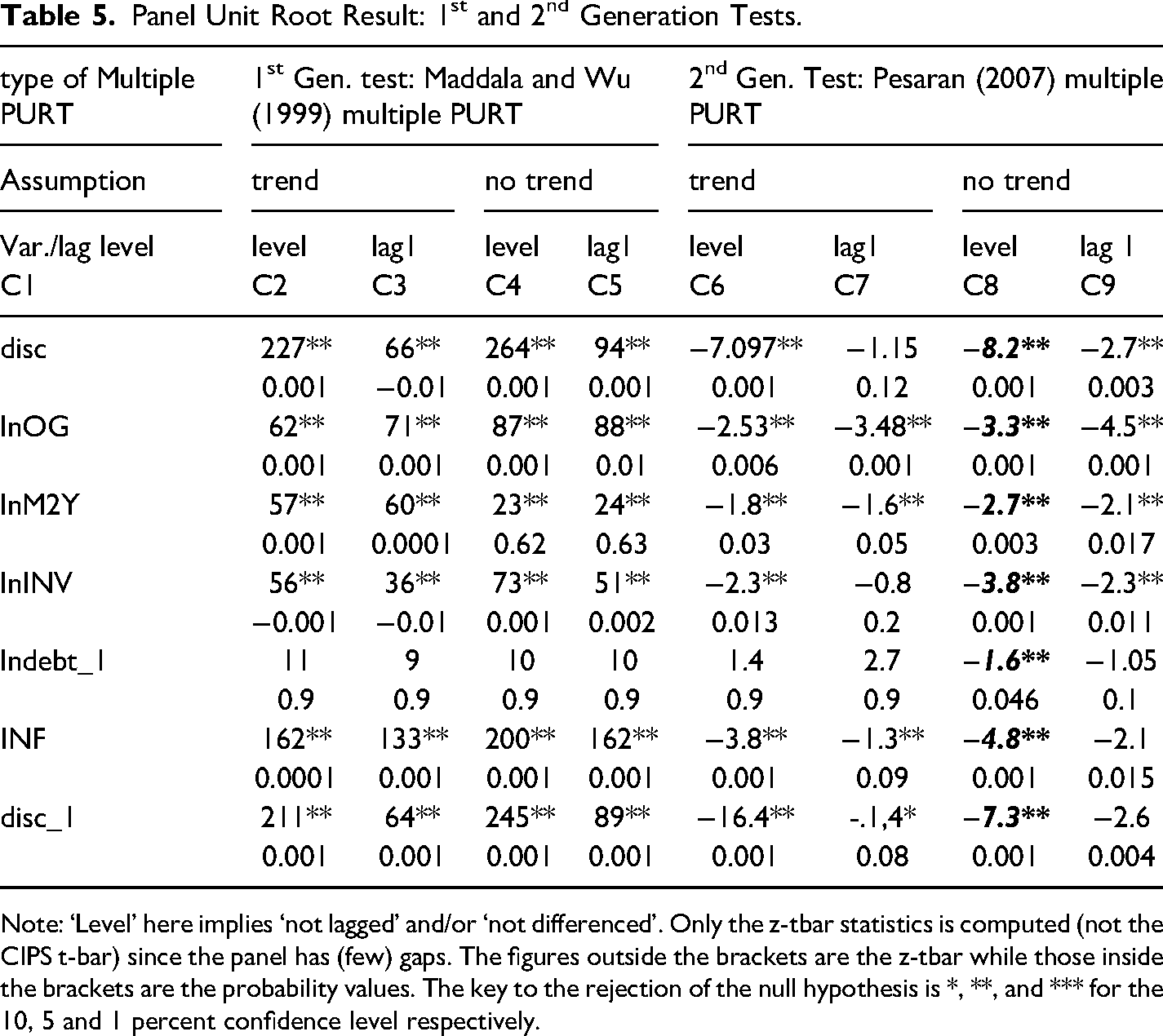
Note: ‘Level’ here implies ‘not lagged’ and/or ‘not differenced’. Only the z-tbar statistics is computed (not the CIPS t-bar) since the panel has (few) gaps. The figures outside the brackets are the z-tbar while those inside the brackets are the probability values. The key to the rejection of the null hypothesis is , , and for the 10, 5 and 1 percent confidence level respectively.

As noted, given the ability of the second-generation test to also account for potential heterogeneity in panels (in addition to accounting for cross-sectional dependency), we rely on the Pesaran test for the conclusion regarding the integration properties of our dataset. Markedly too, although the level values of ‘debt’ become stationary after differencing (not reported), its ‘log’ and its ‘lag1-log’ became stationary without differencing, i.e., its ‘log’ and ‘the first lag of its log’ are stationary just like its first difference. Our result thus clearly shows that in addition to differencing, the use of ‘log’ and ‘lag-log’ transformations are additional ways of inducing stationarity in potentially non-stationary time series (see Baltagi, 2008). We, therefore, conclude that the specific forms (log and lag) of our variables (in C8) are ideal for the implementation of a fixed-effect regression model; this simply implies that the variables (in their log and lag) can be safely included in our baseline fixed-effect model without fear of obtaining spurious regression result that could arise if our variables were otherwise non-stationary.

Finally, the next result we present is that of the fixed-effect model. Table 6 shows the result of the fixed effect panel data regression estimated for the 14 ECOWAS Countries in our sample.

Table 6.
Fixed Effect Result for the Pre-Convergence, Convergence Era and Full Period in ECOWAS.

Sample: 14 ECOWAS Countries

Pre-CC Era (1995–2002) Eq.5 CC Era (2003–2018) Eq.5 Full Year (1995–2018) Eq.6

Regressor C2 C3 C4

OG_1 0.2 −8.33 −0.1

(0.76) (0.00001)** (0.4)

logM2Y 14.9 20.22 0.78

(0.54) (0.53) (0.61)

logINV −20.5 3.15 −0.6

(0.097) ((0.8) (0.9)

Debt_1 −0.24 −0.19 −0.2

(0.03) (0.42) (0.03)

INF −0.32 3.86 0.1

(0.6) (0.012)** (0.1)

DISC_1 −0.30 −0.27 −0.2

(0.015) (0.00001) (0.001)

id1 − − −0.83

− − (0.001)

Intercept 39.5 −90.1 3.0

(0.58) (0.4) (0.5)

corr(u_i, Xb) −0.41 −0.46 −0.53

F value 2.37 6.3 3.07

Prob > F 0.04 0.00001 0.06

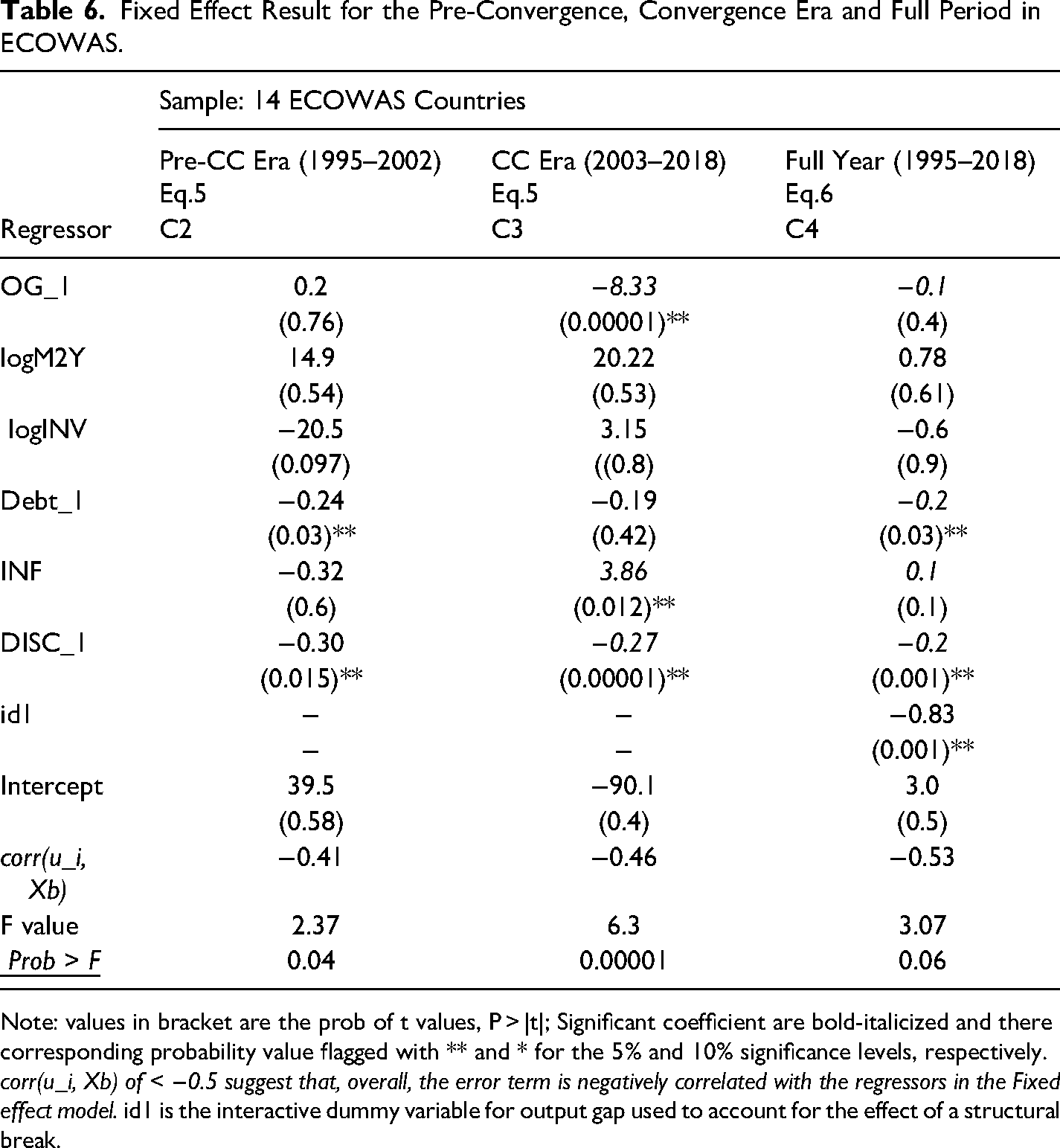
Note: values in bracket are the prob of t values, P > |t|; Significant coefficient are bold-italicized and there corresponding probability value flagged with ** and * for the 5% and 10% significance levels, respectively. corr(u_i, Xb) of < −0.5 suggest that, overall, the error term is negatively correlated with the regressors in the Fixed effect model. id1 is the interactive dummy variable for output gap used to account for the effect of a structural break.

The first column reports the list of regressors included in the baseline model (equation 5). Columns C2 and C3 report the result for the pre-convergence era (1995–2002) and the Convergence era (2003–2018). In column C4, we report the result for the entire/full-year period (1995–2018) estimated with the modified baseline equation (eq.6) that accounts for structural break in the FE model. Since part of our objectives in this study focuses on whether there is a detectable change in the value (sign, magnitude, and significance) of a₁, we also focus our discussion on the fiscal policy reaction to output gap. In addition, we carefully discuss the sign, size and significance of the lagged external debt stock and lagged discretionary deficit included in the model as well as other explanatory variables in the model.

More precisely, if the macroeconomic convergence criteria adopted in ECOWAS effectively -prevented the economies from engaging in counter-cyclical fiscal policy-making, one would expect an increase in the value of the coefficient, a₁, and possibly a sign switch from a ‘negative’ coefficient (representing counter-cyclicality) to ‘positive’ coefficient (representing pro-cyclicality).

Beginning with the pre-convergence era, the coefficient of output gap (a₁) is found to be positive (0.2) but insignificant (with a p-value of 0.76). The positive coefficient suggests that fiscal policy is mildly pro-cyclical before the convergence criteria were adopted in most ECOWAS countries in 2002. On the other hand, the coefficient of a₁ in the convergence era is negative (−8.3) and highly significant (with a p-value of 0.00001) – suggesting that fiscal policy is basically counter-cyclical in the macroeconomic convergence period in ECOWAS. The result of the full-year period suggests that fiscal policy is mildly counter-cyclical with a coefficient of −0.1 (but insignificant). Expectedly, the significance (and absolute size too) of a₁ for the full year declined in relation to the convergence era suggesting that counter-cyclicality in the full year may have been attenuated by the observed pro-cyclicality in the pre-convergence period. Taken in absolute terms, the size of the coefficient also plummeted from −8.33 to −0.1 which buttresses a possible ‘attenuation effect’ arising from the observed pro-cyclicality in the pre-convergence period

Overall, concerning the pro-cyclical behaviour of fiscal policy, what the FE result indicates is that although policymakers set fiscal policy counter-cyclically in the convergence period – a result that remains robust for the convergence period and full-year period – the latter is less counter-cyclical relative to the former. The decline in counter-cyclicality in the full-year period may have resulted from an ‘attenuation effect’ arising from the pro-cyclical nature of fiscal policy in the pre-convergence period which is part of the full-year period. To be clear, we did not find any evidence in support of the presumption that the convergence criteria may have become an unnecessary strait-jacket on national fiscal policymaking in ECOWAS economies. If anything, we found evidence to the contrary. Fiscal policy has been more counter-cyclical following the adoption of the convergence criteria.

Looking at the respective coefficients of initial/past debt and discretionary deficit, a₄ and a₆, we earlier noted that a value of a₄ that is negative or an a₆ that is less than 1 implies that the higher the initial debt, or the higher the initial deficit, the lower the discretionary deficit that policymakers set discretionally. As Table 6 shows, fiscal policy responded negatively to past debt and past deficit in the pre-convergence criteria era in ECOWAS. For instance, the respective coefficients of past debt and past deficit are −0.24 and −0.3 in the pre-convergence. This suggests that policymakers in ECOWAS respond to initial conditions (debt and deficit). There is, thus, evidence that fiscal policymaking in the pre-convergence era could be one that simply takes clue from past (initial) debt and past deficit rather than one that focuses explicitly on achieving a rule-based fiscal benchmark such as the one set by the convergence criteria. This appears to be particularly the case because as the coefficient of output gap in the pre-convergence era shows, fiscal policy was pro-cyclical during the period but switch to counter-cyclical in the convergence era.

Markedly, our findings that policymakers in ECOWAS simply take clue from initial debt and deficit in the absence of fiscal rules (or when rule exist but are not binding) is clearly seen to extend well beyond the pre-convergence era. This is shown by the fact that a₄ and a₆ remained negative during the convergence era. Importantly, this result is also found to remain robust to the full year specification after accounting for the potential effect of a structural break in the model. However, this may not be too surprising because one would expect this result where and when fiscal rules either do not exist or exist but are not binding. In fact, as has earlier been noted, the macroeconomic fiscal rules in ECOWAS are bound to fail no matter how elegant or elaborate they have been designed, except if they become binding. This, of course, explains why the most elaborate fiscal rule so far designed in the world (the Stability and Growth Pact, SGP) failed, i.e., the SGP (which provides concrete contents to the Maastricht Treaty) failed because the rules were not binding although they included sanction which was merely designed as atomic bombs – never to be applied.

Zooming in on the basic matter of structural change in our panel data model, the output-gap interactive dummy variable indicates how, on average, fiscal policy responded to our model variable or variables (here output gap) in the convergence period compared to the pre-convergence period. In specifics, taking the face value, the coefficient of 0.83 for the output-gap dummy indicates that for any unit change in fiscal benchmark, policymakers responded in a systematic counter-cyclically manner by 0.83 in the convergence period compared to pre-convergence period. This coefficient is also found to be significant with a p-value of 0.001 indicating a shift to counter-cyclical behaviour in the convergence period.

To be clear, we do not claim that the observed counter-cyclicality in the convergence period is the result/consequence of the benchmark imposed by the fiscal rules of the convergence criteria. In order words, we do not claim that countries that utilize discretionary fiscal policy (necessarily) do so because of the constraints imposed by the convergence criteria. What our result clearly shows is that the constraints associated with the convergence criteria have not made fiscal policy less countercyclical. Instead, we found that fiscal policy has been more counter-cyclical in the convergence period in ECOWAS. Whether the observed counter-cyclicality is a result (consequence) of the constraints associated with the convergence criteria or of other factors or– in indeed, a rationale for it –remains unclear and, perhaps, a subject of further research.

Overall, the observed shift from pro-cyclical (in pre-convergence era) to counter-cyclical (in convergence period) regarding fiscal policymaking in ECOWAS countries is a result that closely aligns with the findings for the EU countries. In the EU, fiscal policy was found to be generally pro-cyclical in the pre-Maastricht European Monetary Union era (1980–1991) but turned out to be counter-cyclically in the post-Maastricht European Monetary Union era (1992–2002) (see Gali et al., 2003, p. 548 for a discussion).

Conclusions and Lessons for Policy

The macroeconomic convergence criteria have been described as an unnecessary straightjacket that can hamper the ability and motivation of ECOWAS countries to stabilize their economies through active counter-cyclical fiscal policy.¹⁸ This study tests the empirical merit of this assertion. In specifics, we investigate whether and how the convergence related constraints may have made fiscal policy pro-cyclical in ECOWAS and how the countries in the region may have used discretionary fiscal policy as a stabilizing tool over the past two decades.

The study relies on the Fixed effect (FE) model estimated separately for the pre-convergence period (1995–2002), the convergence era (2003–2018), and the full year (1995–2008) for the 14 ECOWAS economies in our sample. We test the existence of structural break in our panel data model and account for it in the full year specification using and interactive output-gap dummy. As we are interested in testing whether the constraint on fiscal policy associated with the convergence criteria (CC) effectively constrained counter-cyclical policymaking in ECOWAS countries, we investigate whether there is a significant change in the coefficient of the output gap (a1) in the Convergence period (2003–2018) in relation to the pre-convergence era (1995–2002) in ECOWAS countries.

The key results are as follows: (i) we found a switch from pro-cyclical fiscal policymaking in the pre-convergence era (1995–2002) to counter-cyclical fiscal policymaking in the convergence era (2003–2018) in ECOWAS. This result appears to align with past trend in the European Union where fiscal policy was found to be mildly pro-cyclical in the pre-Maastricht EMU era (1980–1991) but turned out to be counter-cyclically in the post-Maastricht EMU era (1992–2002); (ii) the size and significance of the coefficient representing output gap (a₁) declined (for the full-year result) suggesting that counter-cyclicality in the full year may have been attenuated by our earlier finding of pro-cyclicality in the pre-convergence period; (iii) discretionary fiscal policy responded negatively to initial debt and initial deficit suggesting that fiscal policymaking in the pre-convergence era could be one that simply takes clue from initial debt and initial deficit rather than one that focuses explicitly on achieving a rule-based fiscal benchmark/target such as the one set by the convergence criteria.

In conclusion, we make no claim that the countries that utilize discretionary fiscal policy do so because of the constraints imposed by the convergence criteria. What our result clearly shows is that the constraints associated with the convergence criteria have not made fiscal policy less countercyclical. Instead, we found evidence to the contrary. In particular, fiscal policy has been more counter-cyclical in the convergence period in ECOWAS. As noted, whether the observed counter-cyclicality is a result (consequence) of the constraints associated with the convergence criteria or of other factors or– in indeed, a rationale for it –remains a subject of further research. Most interestingly, from our finding that policymakers apparently take clue from initial deficit and debt is setting discretionary fiscal policy in both the pre-convergence and convergence periods in ECOWAS, the switch to counter-cyclical fiscal policymaking in the convergence period may not be uncorrelated with the constraints imposed by the fiscal rules.

Policy Lessons

From the above insightful results of the study, the following key policy lessons could be gleaned:

(i) Account for Business Cycle in setting Discretionary Policy: Our finding – against the presumption of the dissenting viewpoint regarding the structure of monetary union arrangement in ECOWAS – that discretionary fiscal policy has actually been countercyclical in the convergence period clearly suggest the need to introduce more flexibility in fiscal policymaking through discretionary fiscal policy that endeavours to balance the budget (against the constraints imposed by the convergence rules) over the business cycle.

(ii) Promote Sound Borrowing Policies: Our finding of a clear trend towards a decline in the coefficient of output gap in the convergence era relative to the pre-convergence era not only suggests a drive towards counter-cyclical fiscal policymaking for countries in the region but also the potential to improve compliance with the convergence criteria. And so, national governments in ECOWAS should harness this potential by accelerating the implementation of different legal instruments adopted by the Community such as the promotion of sound borrowing policies.

(iii) Adopt the use of Discretionary Fiscal Policy to monitor Compliance: The use of discretionary fiscal policy (a departure from the tradition of relying on the total fiscal deficit) should be adopted by the Convergence Council in monitoring compliance with the Convergence criteria. This is necessary to adequately capture action taken to correct excessive deficit.

Variable	Code	Description	Source
Debt Stock	DS	External Debt Stock, total (DOD, current US$)	WDI (current US$)
Debt/GNI	DEBT	External debt stocks (% of GNI)	WDI
Gross Domestic Price	GDP	Real GDP (Constant 2010 US Dollar)	WDI (2010 Const. US$)
General government revenue (LCU’ b)	GR	Revenue consists of taxes, social contributions, grants receivable, and other revenue. Revenue increases the government’s net worth, which is the difference between its assets and liabilities (GFSM 2001, paragraph 4.20). Note: Transactions that merely change the composition of the balance sheet do not change the net worth position, for example, proceeds from sales of nonfinancial and financial assets or incurrence of liabilities.	WEO (bil. of LCU)
General government total expenditure (LCU’ b)	GE	Total expenditure consists of total expense and the net acquisition of nonfinancial assets. Note: Apart from being on an accrual basis, total expenditure differs from the GFSM 1986 definition of total expenditure in the sense that it also takes the disposals of nonfinancial assets into account.	WEO (bil. of LCU)
General Government Expenditure(% GDP)	GEY	General Government Expenditure(% GDP)	WEO
General Government Revenue (% GDP)	GRY	General Government Revenue (% GDP)	WEO
Total Fiscal Deficit (LCU’ b)	fDef	General Govt. total Expenditure less General Govt. Total Revenue	WEO
Discretionary Deficit	DISC	discretionary deficit is computed using the formula in equation 4 (see eqt 4; Mourre et al., 2013).	WEO
Output Gap	OG	Computed using the formula: (cyclical GDP/Potential GDP)*100. Both the cyclical GDP and potential GDP are obtained from the rea;l GDP data using HP filter (see eq. 1, 2and 3)	WEO

	Sample: 14 ECOWAS Countries
OG_ ₁	−0.66	−0.86
logM2Y	11.8	15
log INV	−12.3	−3.54
DEBT_ ₁	−0.09	−0.11
INF	0.098	2.52
DISC_ ₁	−0.1856	−0.03
chi2(1)	29.77	7.7
Prob_chi2	0.00001	0.025

type of Multiple PURT	1^st Gen. test: Maddala and Wu (1999) multiple PURT	2^nd Gen. Test: Pesaran (2007) multiple PURT
disc	227**	66**	264**	94**	−7.097**	−1.15	−8.2**	−2.7**
	0.001	−0.01	0.001	0.001	0.001	0.12	0.001	0.003
lnOG	62**	71**	87**	88**	−2.53**	−3.48**	−3.3**	−4.5**
	0.001	0.001	0.001	0.01	0.006	0.001	0.001	0.001
lnM2Y	57**	60**	23**	24**	−1.8**	−1.6**	−2.7**	−2.1**
	0.001	0.0001	0.62	0.63	0.03	0.05	0.003	0.017
lnINV	56**	36**	73**	51**	−2.3**	−0.8	−3.8**	−2.3**
	−0.001	−0.01	0.001	0.002	0.013	0.2	0.001	0.011
lndebt_1	11	9	10	10	1.4	2.7	−1.6**	−1.05
	0.9	0.9	0.9	0.9	0.9	0.9	0.046	0.1
INF	162**	133**	200**	162**	−3.8**	−1.3**	−4.8**	−2.1
	0.0001	0.001	0.001	0.001	0.001	0.09	0.001	0.015
disc_1	211**	64**	245**	89**	−16.4**	-.1,4*	−7.3**	−2.6
	0.001	0.001	0.001	0.001	0.001	0.08	0.001	0.004

	Sample: 14 ECOWAS Countries
OG_1	0.2	−8.33	−0.1
	(0.76)	(0.00001)**	(0.4)
logM2Y	14.9	20.22	0.78
	(0.54)	(0.53)	(0.61)
logINV	−20.5	3.15	−0.6
	(0.097)	((0.8)	(0.9)
Debt_1	−0.24	−0.19	−0.2
	(0.03)**	(0.42)	(0.03)**
INF	−0.32	3.86	0.1
	(0.6)	(0.012)**	(0.1)
DISC_1	−0.30	−0.27	−0.2
	(0.015)**	(0.00001)**	(0.001)**
id1	−	−	−0.83
	−	−	(0.001)**
Intercept	39.5	−90.1	3.0
	(0.58)	(0.4)	(0.5)
corr(u_i, Xb)	−0.41	−0.46	−0.53
F value	2.37	6.3	3.07
Prob > F	0.04	0.00001	0.06

Footnotes

Declaration of Conflicting Interests

The author(s) declared no potential conflicts of interest with respect to the research, authorship, and/or publication of this article.

Funding

The author(s) disclosed receipt of the following financial support for the research, authorship, and/or publication of this article: This work was supported by the Consortium pour la recherche économique en Afrique, (grant number RT19501).

ORCID iD

Kenneth Onye

Notes

Appendix Summary and Descriptive Statistics of Convergence Variables in ECOWAS: Tables A1–A6,A8

References

Afonso

(2000). Fiscal Policy Sustainability: Some Unpleasant European Evidence. ISEG Working Paper No. 12/2000/DE/CISEP. SSRN: https://ssrn.com/abstract=317483or https://doi.org/10.2139/ssrn.317483.

Afonso, A., & Furceri, D. (2010). Government size, composition, volatility and economic growth. European Journal of Political Economy, 26, 517–532. https://dx-doi-org.web.bisu.edu.cn/10.1016/j.ejpoleco.2010.02.002.

Afonso

Rault

(2010). What do we really know about fiscal sustainability in the EU? A panel data diagnostic. Weltwirtschaftliches Archiv, 145(4), 731–755. https://doi.org/10.1007/s10290-009-0034-1

Alagidede

Tweneboah

(2015). On the sustainability and synchronization of fiscal policy in Latin America. Latin American Journal of Economics, 52(5), 213–240. https://dx-doi-org.web.bisu.edu.cn/10.7764/LAJE.52.2.213

Alby

(2018). CFA Franc: A new stress test. Eco Conjuncture, Economic-Research. Bnpparibas.com.

Alesina

Campante

Tabellini

(2008). Why is fiscal policy often procyclical? Journal of the European Economic Association, 6(5), 1006–1036. https://doi.org/10.1162/JEEA.2008.6.5.1006

Allsopp

Vine

(1996). Fiscal policy and EMU. Economic Review, 158, 91–107. https://doi.org/10.1177/002795019615800107

Arai

(2011). Productive government expenditure and fiscal sustainability. Finanz-archiv, 67(4), 327–351. https://doi.org/10.1628/001522111X614150

Areaza

Sorensen

B. E.

Yosha

(1999). Consumption smoothening through fiscal policy in OECD and EU countries. In Poterba

J. M.

von Hagen

(Eds.), Fiscal institutions and fiscal performance (pp. 59–80). University of Chicago Press.

10.

Auerbach (2002). Is there a role of discretionary fiscal policy? In rethinking stabilization policies. Federal Reserve Bank of Kansas City, 109–150. Retrieved from https://ideas.repec.org/a/fip/fedkpr/y2002p109-150.html

11.

Ballabriga

Martinez-Mongay

(2002). Has EMU shifted policy? Economic Papers, European Commission, Directorate-General for Economic and Financial Affairs, No. 166. http://europa.eu.int/comm/economy-finance.

12.

Baltagi

(2008). Econometric analysis of panel data. John Wiley & Sons.

13.

Bohn

(1998). The behavior of U.S. public debt and deficits. The Quarterly Journal of Economics, 113(3), 949–963. https://doi.org/10.1162/003355398555793

14.

Central Bank of Iceland (2005). Monetary Bulletin.

15.

Chang

Liu

W. R.

Thompson

(2002). The viability of fiscal policy in South Koria, Taiwan, and Thailand. ASEAN Economic Bulletin, 19(2), 170–177. https://doi.org/10.1355/AE19-2D

16.

Chong

Jorda

Taylor

A. M.

(2012). The Harrod-Balassa-Samuelson hypothesis: real EXCHANGE rate and their long run equilibrium. International Economic Review, 53(2), 609–634. https://doi.org/10.1111/j.1468-2354.2012.00694.x

17.

Choudhary

Hanif

Iqbal

(2013). On smoothing macroeconomic time series using HP and modified HP filter. State Bank of Pakistan, 46(19), 2205–2214. 10.1080/00036846.2014.894631.

18.

Darby

McIntyre

(2018). The output gap: What is it, how can it be estimated and are estimates fit for policymakers’ purposes? Economic Commentary, June 2018. Retrieved from https://strathprints.strath.ac.uk/64530/

19.

Debrun

Masson

Pattilo

(2005). Monetary union in West Africa: Who might gain, who might lose, and why? Canadian Journal of Economics/Revue Canadienne d`Economique, 38(2), 454–481. https://doi.org/10.1111/j.0008-4085.2005.00288.x

20.

ECOWAS Macroeconomic Convergence (2010). Report on the macroeconomic convergence of member states of the economic community of West African states (ECOWAS) in 2010. ECOWAS Commission.

21.

ECOWAS Macroeconomic Convergence Report (2016). ECOWAS Convergence report 2016. ECOWAS Commission.

22.

Egwaikhide

F. O.

Ogunleye

E. K.

(2010). Globalization and macroeconomic convergence criteria in the West African monetary zone. Journal of Monetary and Economic Integration, 10(1), 89–102.

23.

Ekpo

A. H.

(2018). Economic Integration In West Africa: A Reconsideration Of The Evidence. A paper presented at the American Economic Association, (AEA), African Finances Economic Association (AFEA) and the National Economic Association (NEA), Atlanta, Georgia, January 4–1, 2018.

24.

Eyraud

Liedo

V. D.

Dudine

Peralda

(2018). How to select fiscal rules: A primer. IMF FAD.

25.

Fatas

Mihov

(2002). On Constraining fiscal Policy and EMU, mimeo, INSEAD.

26.

Fatas

Mihov

(2003a). On constraining fiscal policy discretion in EMU. Oxford Review of Economic Policy, 19(1), 112–131. https://doi.org/10.1093/oxrep/19.1.112

27.

Fatas

Mihov

(2003b). The case for restricting fiscal policy discretion, mimeo. INSEAD and CEPR, 118(4), 1419–1447. https://doi.org/10.1162/003355303322552838

28.

Fatás

Mihov

(2001). The effects of fiscal policy on consumption and employment: theory and evidence. INSEAD and CEPR.

29.

Fedelino

Ivanova

Horton

(2009). Computing cyclically adjusted balances and automatic stabilizers. Fiscal Affairs Department, International Monetary Fund, 2009(5). https://doi.org/10.5089/9781462359622.005

30.

Gali

Perotti

Lane

P. R.

Richter

W. F.

(2003). Fiscal policy and monetary integration in Europe. Economic Policy, 18(37), 533–572. https://doi.org/10.1111/1468-0327.00115_1

31.

Hercowitz

Strawczynski

(1999). Cyclical bias in government spending: Evidence from the OECD. Tel Aviv University.

32.

Hodrick

R. J.

Edward

C. P.

(1997). Postwar U.S. Business cycles: an empirical investigation. Journal of Money, Credit and Banking, Ohio State University Press, 29(1), 1–16. https://doi.org/10.2307/2953682

33.

International Monetary Fund (2018). Sub-Saharan Africa: Domestic Revenue Mobilization and Private Investment. Regional Economic Outlook, World economic and financial surveys, Washington, DC, April.

34.

Jebuni

C. D.

Ogunkola

E. O.

Soludo

C. C.

(1999). A review of regional integration experience in Sub-Saharan Africa: A case study of the economic community of West African states. In Oyejide

T. A.

(Ed.), Regional integration and trade liberalization in sub-saharan Africa, volume 3. Longman.

35.

Kydland

F. E.

Prescot

E. C.

(1977). Rules rather than discretion: the inconsistency of optimal plans. The Journal of Political Economy, 85(3), 473–491. https://doi.org/10.1086/260580

36.

Lane

(2002). The cyclical behaviour of Fiscal policy: evidence from the OECD. Journal of Public Economics, 87(12), 2661–2675. https://doi.org/10.1016/S0047-2727(02)00075-0

37.

Lee

Sung

(2007). Fiscal policy, business cycles and economic stabilisation: Evidence from industrialized and developing countries. Fiscal Studies, 28(4), 437–462. https://doi.org/10.1111/j.1475-5890.2007.00063.x

38.

Maddala

G. S.

(1999). A comparative study of unit root tests with panel data and a new simple test. Oxford Bulletin of Economics and Statistics, Special Issue, 61(1), 631–652. https://doi.org/10.1111/1468-0084.0610s1631

39.

Martin-Baillon

(2018). Business Cycle Facts, TA Session.

40.

Martinez-Mongay, C. (2002). Fiscal policy and the size of governments. In M. Buti, J. von Hagen, & C. Martinez-Mongay (Eds.), The behavior of fiscal authorities. Stabilization, Growth and Institutions (Chapter 5). Palgrave.

41.

Mbaye

Badia

M. M.

Chae

(2018). Bailing Out the People? When Private Debt Becomes Public. IMF Working Paper WP/18/141.

42.

Mélitz

(1997). Some Cross-Country Evidence about Debt, Deficits, and the Behaviour of Monetary and Fiscal Authorities. CEPR Discussion Paper No.1653.

43.

Mourre

Isbasoiu

Paternoster

Salto

(2013). The cyclically adjusted budget balance used in the EU Fiscal framework: An update. Economic Papers, 478. https://doi.org/10.2765/3922

44.

Pesaran

M. H.

(2007). A simple panel unit root test in the presence of cross-section dependence. Journal of Applied Econometrics, 22(2), 265–312. https://doi.org/10.1002/jae.951

45.

Prohl

Westerlund

(2009). Using panel data to test for fiscal sustainability within the European Union. Public Finance Analysis, 65(2), 246–269. https://doi.org/10.1628/001522109X470612

46.

Qureshi

M. S.

Tsangarides

(2006). What is Fuzzy About Clustering in West Africa? IMF Working Paper WP/06/90, March 2006.

47.

Saka

J. O.

Onafowokan

I. A.

Adebayo

A. A.

(2015). Analysis of convergence criteria in a proposed monetary union: A study of the economic community of West African States. International Journal of Economics and Financial Issues, 5, 230–239.

48.

Seck

(2013). Fifteen Years of WAEMU: Results and Strategies for the Future, Chapter 2.

49.

Sissoho

Ahotor

C. R.

Odeniran

O. S.

Nyako

Haffner

Adams

(2015). The Greek debt crisis: Lessons for the ECOWAS single currency project. WAMI Occasional Paper Series, 1(8), 1–31. http://hdl.handle.net/10419/264219

50.

Svensson

L. E. O.

(2003). What is wrong with Taylor rules? Using judgment in monetary policy through targeting rules. Journal of Economic Literature, 41(2), 426–477. https://doi.org/10.1257/.41.2.426

51.

Tarawalie

A. B.

Sissoho

Conte

Ahotor

C. R.

(2013). Fiscal and monetary policy coordination in the WAMZ: Implications for member States’ performance on the convergence criteria. WAMI Occasional Paper Series, 1(4), 1–45. Retrieved from http://hdl.handle.net/10419/264215

52.

Tarawalie

A. B.

Sissoho

Conte

Ahotor

C. R.

(2014). Political business cycle and macroeconomic convergence: The WAMZ experience. WAMI Occasional Paper Series, 1(7), 1–40. Retrieved from http://hdl.handle.net/10419/264218

53.

Ter-Minassian

(2010). Preconditions for a successful introduction of structural fiscal balance-based rules in latin america and the caribbean: A framework paper. Inter-American Development Bank Discussion Paper, No. IDB-DP-157.

54.

Whittaker

E. T.

(1923). On a new method of graduation. Proceedings of the Edinburgh Mathematical Association, 41(78), 63–75. https://doi.org/10.1017/S0013091500077853; corpus id: 120579706

55.

World Development Indicators (2019). World Bank’s World Development Indicators Database 2019. Accessed November 2019 at https://databank.worldbank.org/reports.aspx?source=World-Development-Indicators.

56.

World Economic Outlook (2019). IMF World Economic Outlook Database. Accessed April 2019 at https://www.imf.org/external/pubs/ft/weo/2018/01/weodata/index.aspx.

57.

Wyplosz

(2002). Fiscal discipline in EMU: Rules or institutions? Mimeo, Graduate Institute for International Studies.

58.

Wyplosz

(2005). Fiscal policy: institutions versus rules. National Institute Economic Review, 191(1), 64–78. https://doi.org/10.1177/0027950105052661

	Sample: 14 ECOWAS Countries
C1	C2	C3
C1	Pre-CC Era(1995–2002)	CC Era(2003–2018)
Regressor	(b-B)	(b-B)
OG_ ₁	−0.66	−0.86
logM2Y	11.8	15
log INV	−12.3	−3.54
DEBT_ ₁	−0.09	−0.11
INF	0.098	2.52
DISC_ ₁	−0.1856	−0.03
chi2(1)	29.77	7.7
Prob_chi2	0.00001	0.025

type of Multiple PURT	1^st Gen. test: Maddala and Wu (1999) multiple PURT				2^nd Gen. Test: Pesaran (2007) multiple PURT
Assumption	trend		no trend		trend		no trend
Var./lag level	level	lag1	level	lag1	level	lag1	level	lag 1
C1	C2	C3	C4	C5	C6	C7	C8	C9
disc	227**	66**	264**	94**	−7.097**	−1.15	−8.2**	−2.7**
	0.001	−0.01	0.001	0.001	0.001	0.12	0.001	0.003
lnOG	62**	71**	87**	88**	−2.53**	−3.48**	−3.3**	−4.5**
	0.001	0.001	0.001	0.01	0.006	0.001	0.001	0.001
lnM2Y	57**	60**	23**	24**	−1.8**	−1.6**	−2.7**	−2.1**
	0.001	0.0001	0.62	0.63	0.03	0.05	0.003	0.017
lnINV	56**	36**	73**	51**	−2.3**	−0.8	−3.8**	−2.3**
	−0.001	−0.01	0.001	0.002	0.013	0.2	0.001	0.011
lndebt_1	11	9	10	10	1.4	2.7	−1.6**	−1.05
	0.9	0.9	0.9	0.9	0.9	0.9	0.046	0.1
INF	162**	133**	200**	162**	−3.8**	−1.3**	−4.8**	−2.1
	0.0001	0.001	0.001	0.001	0.001	0.09	0.001	0.015
disc_1	211**	64**	245**	89**	−16.4**	-.1,4*	−7.3**	−2.6
	0.001	0.001	0.001	0.001	0.001	0.08	0.001	0.004

	Sample: 14 ECOWAS Countries
	Pre-CC Era (1995–2002) Eq.5	CC Era (2003–2018) Eq.5	Full Year (1995–2018) Eq.6
Regressor	C2	C3	C4
OG_1	0.2	−8.33	−0.1
	(0.76)	(0.00001)**	(0.4)
logM2Y	14.9	20.22	0.78
	(0.54)	(0.53)	(0.61)
logINV	−20.5	3.15	−0.6
	(0.097)	((0.8)	(0.9)
Debt_1	−0.24	−0.19	−0.2
	(0.03)**	(0.42)	(0.03)**
INF	−0.32	3.86	0.1
	(0.6)	(0.012)**	(0.1)
DISC_1	−0.30	−0.27	−0.2
	(0.015)**	(0.00001)**	(0.001)**
id1	−	−	−0.83
	−	−	(0.001)**
Intercept	39.5	−90.1	3.0
	(0.58)	(0.4)	(0.5)
corr(u_i, Xb)	−0.41	−0.46	−0.53
F value	2.37	6.3	3.07
Prob > F	0.04	0.00001	0.06

Fiscal Policy and Monetary Integration in the Ecowas

Abstract

Keywords

Introduction

Stylized Facts on ECOWAS & the Political Economy of Poor Convergence

Macroeconomic Convergence Status in ECOWAS (2004–2018) 6

The Cyclicality of Output Gap and Dynamics of Debt and Deficit (1995–2018)

Dynamics of Cyclical, Potential and Total Fiscal Deficit in ECOWAS (1995–2018)

Calculating Discretionary Deficit – IMF (and OECD) Approach

Why are ECOWAS Countries not Meeting the CC-A Political Economy Perspective?

Review of Related Literature

Macroeconomic Convergence and Political Business Cycle Literature

Discretionary and Automatic Stabilizer Literature

Methodology

A Priori Expectation

Data Description and Sources

Results and Discussions

Conclusions and Lessons for Policy

Policy Lessons

Footnotes

Declaration of Conflicting Interests

Funding

ORCID iD

Notes

Appendix Summary and Descriptive Statistics of Convergence Variables in ECOWAS: Tables A1–A6,A8

References

Macroeconomic Convergence Status in ECOWAS (2004–2018)⁶