Optimization of hydrofoil leading-edge geometry for delaying incipient cavitation using a CFD

Abstract

Cavitation is a common phenomenon in hydraulic machinery, which brings negative impacts such as noise, vibration, performance drop and material damage into hydraulic turbomachinery. In engineering applications of pumps, the cavitation-free operation is an important issue. Incipient cavitation is the start of cavitation and also a standard to value the cavitation behavior of the pump unit. Improving the incipient cavitation is usually empirical and difficult to conduct.Although previous studies have proposed various geometric modifications and flow control strategies to mitigate cavitation, most approaches are either case-specific or involve trade-offs with hydraulic performance such as efficiency and head. In addition, many studies focus on reducing developed cavitation rather than delaying incipient cavitation, particularly under off-design conditions where pumps are more vulnerable. Furthermore, systematic optimization methods for leading-edge geometry remain limited, and existing approaches often rely on empirical design or local modifications without global search capability. Therefore, there is a need for an efficient and systematic optimization framework to improve incipient cavitation performance while maintaining acceptable hydraulic characteristics. In this study,a NACA0006 hydrofoil is employed as a simplified model to study the delay method of incipient cavitation for pump impellers. The optimization is conducted for specific large incidence angles by using a strategy combined genetic algorithm with computational fluid dynamics. The geometry of hydrofoil is searched in a given range to find a solution which has gentle pressure drop on leading edge separation region. After optimization, new optimized foil profile is found with higher minimum pressure than initial foil. Verified by experiment in cavitation tunnel, the optimized foil is found with a later incipient cavitation and smaller cavity scale than the initial foil at incidence angle around 5 degrees. Based on experimental and numerical analysis, the optimization brings a gentle geometry gradient to hydrofoil by setting target weight values. The optimized geometry causes gentler pressure gradient than initial foil to make the cavitation incepts later and smaller. Very slight changes are found on the Lift/Drag force ratio F_L/F_D which should be carefully checked before applying. For pumps, the optimization method can work to improve the cavitation behavior under off-design conditions and provide a wider cavitation-free operation region in engineering applications.

Keywords

incipient cavitation hydrofoil profile optimization genetic algorithm

1. Introduction

Anti-cavitation design is an enduring issue for the design of hydraulic pumps whose blades are simplified as hydrofoils.^1–8 Cavitation happens in pump unit when pressure somewhere drops below the saturation pressure.⁹ It causes undesirable effects such as vibration, noise, performance decline and material damage.^10–13 There are many different methods for improving the cavitation performance for pumps. It can be mainly classified into two ways. Firstly, reducing the scale and influence of cavitation under a specific operation condition. Secondly, delaying the incipient cavitation for specific operation range. The first way is to improve the distribution of pressure field in the region where cavitation occurs. It is effective for the situation that cavitation scale is already quite large in a designed pump during operation. The second way is to control the lowest pressure where probably suffers cavitation. It works well in the design stage to make a compromise between incipient cavitation performance and other performances.

Many researchers have put forward successful improvements on cavitation performance of pumps and also hydraulic turbines. Yang et al.¹⁴ applied splitter design to pump impeller with reducing of the main blade number. It successfully decreases the cavitation scale in operation range. Yao et al.¹⁵ modified the impeller outlet area of a Francis turbine, reduced the cavitation under the same flow conditions. Luo et al.¹⁶ improved the cavitation performance of centrifugal pump by modifying the leading edge position of impeller blade. These three works increase the flow passage section area where cavitation strongly happens, the cavitation is delayed due to the more spacious place. However, the other performances such as head and efficiency change a lot, further optimizations become necessary. Bosioc et al.¹⁷ introduced a flat free runner jet to prevent the formation of the vortex rope in hydraulic turbines. Motycak et al.¹⁸ and Roussopoulos et al.¹⁹ applied anti-cavitation lip to axial impellers, it is helpful to improve the blade tip clearance cavitation. These two methods are performance-kept but specific for limited cases. There are also researchers who studied the incipient cavitation performance. For pumps, leading edge is important which is both the global lowest pressure region and strong separation region.^20–22 Balasubramanian et al.²³ studies the influence of blade leading edge on cavitation in centrifugal pump. By comparing among blunt, circular, parabola and ellipse leading edge shapes, researchers found that parabola leading edge is the best shape under design condition. Li et al.²⁴ investigated the influence of wavy leading-edge in hydrofoil modification. Results show that the wavy leading-edge can improve the lift-drag characteristics, restrain the hydrofoil cavitation, and reduce the cavitation volume by approximately 30%. Thus, designing a leading edge shape to delay the incipient cavitation or decrease the cavitation scale is possible. However, it is still difficult to find the best shape of leading edge which is anti-cavitation.

For pumps, the leading edge cavitation is triggered due to incidence angle.²⁵ That’s why pumps has only small cavitation or even cavitation-free at design condition. However, cavitation happens much easier at off-design conditions which usually suffer more serious cavitation.²⁶ Therefore, for specific conditions like off-design conditions, the leading edge should be designed with a smaller cavitation or later incipient. Generally speaking, an optimization is necessary in this case. Thus, the design and optimization of hydrofoil profile are studied which helps to find a proper strategy to delay the incipient cavitation for specific conditions. Both the initial and optimized foils are experimentally tested in cavitation tunnel. The optimization method and strategy provide a good solution for anti-cavitation design of pump blades.

2. Solution Strategy

In the quasi-3D-design method,²⁷ the S1 3D-surfaces which are specified spanwise layers between hub and shroud are very important for blade profile design. In Figure 1, one of the S1 3D-surfaces for blade design is shown. There are some important geometric parameters are illustrated including the wrap angle between leading edge and trailing edge Δθ, blade angle on leading edge β_LE, blade angle on trailing edge β_TE and tangential thickness T_B. Usually in centrifugal or mixed-flow cases, θ and β has a differential relationship known as the blade profile differential equation.²⁸ The pump head has also a relationship with the θ and β angles according to the turbomachinery Euler’s equation.²⁹ Therefore, the 3D pump profile can be designed for a particular head requirement by designing θ-β on several specified S1 surfaces.

Figure 1.

Design concept of centrifugal or mixed-flow pump blade on a spanwise layer and the velocity triangles on the blade leading edge.

The tangential thickness T_B has no special configuration in the design concept above. Thus, it is usually designed on a S1 layer with a round or ellipse leading edge which smoothly divide the water between the pressure side and suction side of blade. Starting from leading edge, T_B grows thin-to-thick. The determination of maximum T_B usually compromises the structural strength, fluid passing-ability and manufacturing. Usually, thinner blade is structurally weaker, thicker blade reduces the fluid passing-ability, smooth thickness variation is better for manufacturing. For trailing edge, cut-off, square, ellipse or round types are all feasible.

Figure 1 also shows the velocity triangles on the leading edge of blade of a well-designed impeller. U denotes the rotation velocity of impeller, C denotes the absolute velocity, W denotes the relative velocity, β_LE-f is the relative flow angle. There are three different flow conditions are considered. Under the design load condition, the direction of W is along the blade geometry. Currently, β_LE-f=β_LE. The incoming flow is well-divided by the designed blade profile. Under over load condition, W and C become larger than design load, β_LE-f>β_LE. Consequently, separation becomes severe on the pressure side of blade. Under partial load condition, W and C become smaller than design load, β_LE-f<β_LE. Consequently, separation becomes severe on the suction side of blade. As commonly known in an incompressible flow field, pressure would drop in the separation core region.³⁰ Therefore, pumps usually have worse cavitation performance at off-design conditions, the incipient cavitation is commonly observed on blade leading edge.

Expanding the S1 layer, Figure 2 shows a periodic blade-to-blade view where rotation direction is orthogonal to the streamwise direction. As normally designed, T_B grows thin-to-thick along streamwise direction like a hydrofoil. According to Figure 1, there will be larger separation scale under off-design conditions which require further improvements. T_B on this spanwise layer, regarded as symmetric about the chord line, represents the profile of a hydrofoil. Therefore, T_B strongly influences the flow regime around leading edge and consequently influences the pressure distribution on blade. To improve the incipient cavitation, T_B near leading edge needs modification. Considering the separation region in common pump cases, the control points can be set on the front 5%∼10% of the entire profile as shown in Figure 2.

Figure 2.

Blade-to-blade view of blade profile on a specific spanwise layer.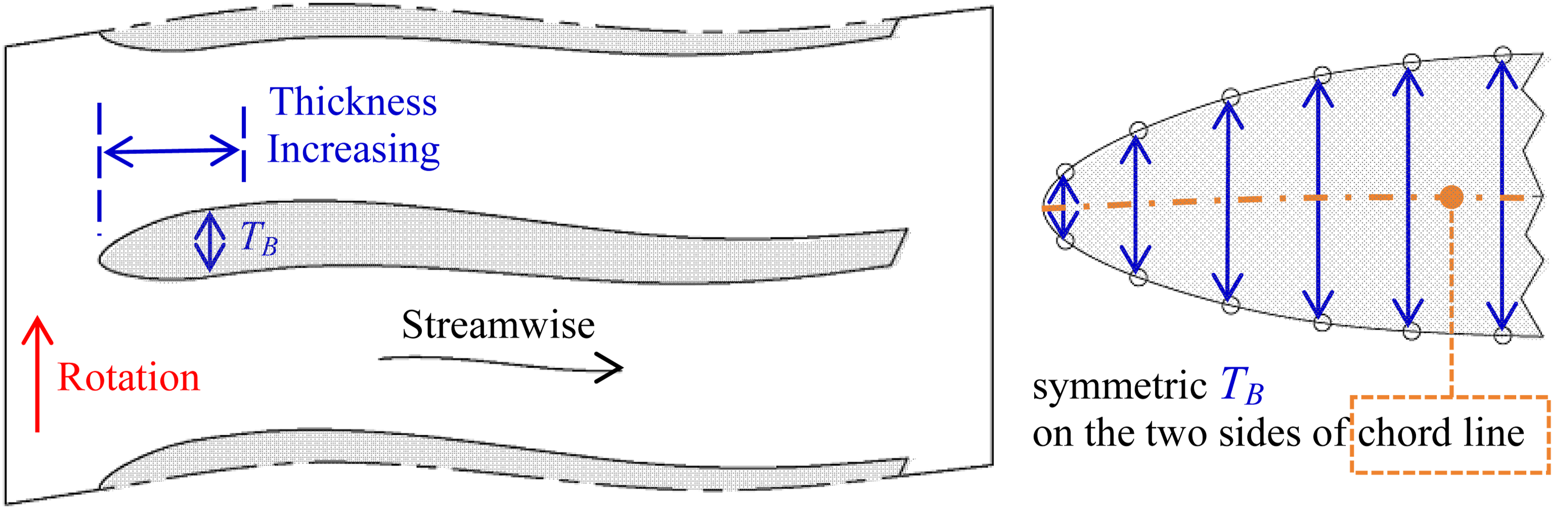

Modifying the T_B on control points and putting forward better cavitation performances are the basic strategy in this study. The Genetic Algorithm (GA) is an evolutionary algorithm popular in engineering optimizations.^31–33 The Computational Fluid Dynamics (CFD) provides good solutions of fitness functions in flow-relevant cases. Thus, GA with CFD solver are compiled as an auto-programming instead of manual testing. Usually, cavitating flow simulation is more time-consumed than single phase flow. A rapid solving process is important for optimization. In this case, the incipient cavitation strongly depends on the lowest-pressure. Therefore, steady state simulation of single phase flow is conducted to solve the value and position of the lowest-pressure instead of incipient cavitation.

3. Application example - NACA0006 hydrofoil

3.1. Geometry of hydrofoil

Hydrofoil, which is a simplified model of turbomachinery blade, are widely used to study the flow mechanism in turbomachinery. In this study, a hydrofoil case study is conducted based on the NACA0006 profile. The NACA0006 hydrofoil is selected as a representative simplified model for turbomachinery blade sections. In quasi-3D pump design, blade profiles on S1 stream surfaces can be locally approximated as hydrofoil-like sections. The symmetric NACA0006 profile provides a well-defined baseline geometry with minimal camber effects, allowing the influence of leading-edge thickness on pressure distribution and cavitation inception to be isolated. Although real pump blades exhibit more complex geometries, the present model is intended to capture fundamental mechanisms rather than reproduce a specific pump configuration.Figure 3 shows the parameters of the NACA0006 profile with an orthogonal L_st-L_sp-T_B coordinate system. L_st denotes the streamwise direction, L_sp denotes the spanwise direction, T_B denotes the foil thickness, T_Bmax=0.06L_st is the maximum thickness which locates 0.3L_st downstream from leading edge. In this study, the last 0.05L_st part is removed to make a cut-off trailing edge. Thus, the foil length along streamwise is actually 0.95L_st.

Figure 3.

Parameters of NACA0006 profile with cut-off trailing edge.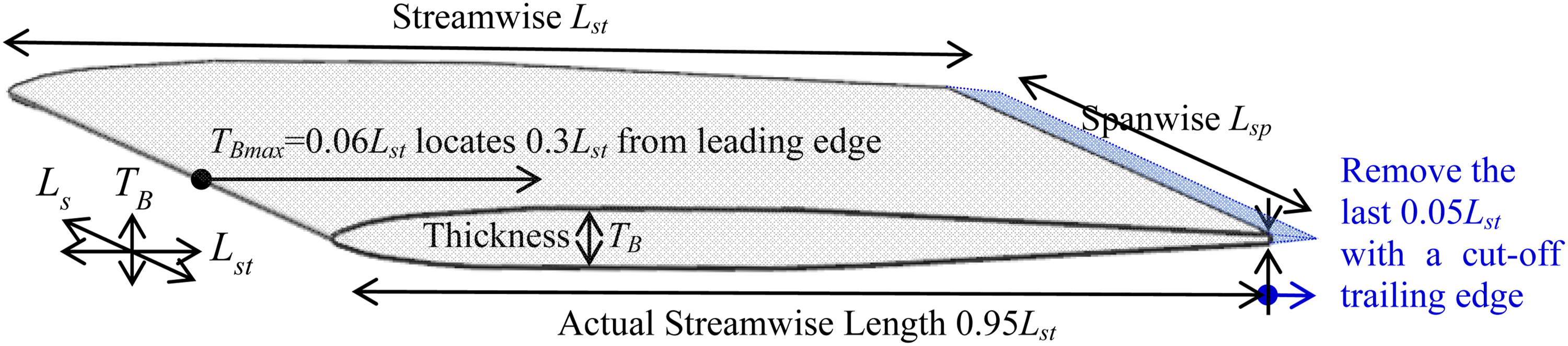

3.2. Parameterization

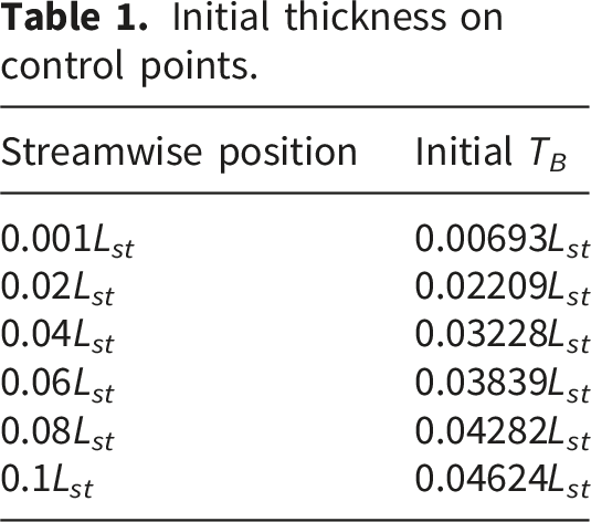
Parameterization is a necessary procedure before optimizationSix control points are distributed within the range of 0.001–0.1 Lst, corresponding to the leading-edge region where flow separation and minimum pressure typically occur. Previous flow analysis (Figure 2) indicates that cavitation inception is highly sensitive to geometric variations in this region. Therefore, the parameterization is concentrated within the first 10% of the chord length to improve optimization efficiency while capturing the dominant physical mechanisms.They are respectively located on 0.001L_st, 0.02L_st, 0.04L_st, 0.06L_st, 0.08L_st and 0.1L_st from leading edge. The thickness on the last control point at 0.1L_st is fixed. Round leading edge is used before 0.001L_st. These control points are geometrically connected using Spline. It should be noted that the number and distribution of control points may influence the optimization outcome. A detailed sensitivity analysis is beyond the scope of the present study and will be addressed in future work.

Constraints are set for the thickness on control points. Firstly, lower limit A and upper limit B are given:

A = \max (T_{B} - 3, 0)

(1)

B = \min (T_{B} + 3, T_{B m a x})

(2)

where the T_B values of initial NACA0006 hydrofoil are listed in Table 1. Secondly, the thickness values should increase progressively along streamwise direction to ensure the smooth of hydrofoil geometry. Each controlled T_B is coded with eight digits’ binary code. The relationship between value and code is:

T_{i - b i n} \to T_{i - d e c}

(3)

T_{i} = a_{i} + T_{i - d e c} \frac{B_{T B i} - A_{T B i}}{2^{8} - 1}

(4)

where T_i-bin denotes the binary code, T_i-dec is the corresponding decimal value of binary code T_i-bin., T_i denotes the actual decimal value of thickness, i denotes the number of parameters. Thus, equation (3) is the binary-decimal conversion. The fixed thickness on 0.1L_st is not parametrized. The other five thickness codes are ordered following i-sequence. Finally, a total 8×5=40 digits’ binary code is generated as the genetic information of each profile sample.

Table 1.

Initial thickness on control points.

Streamwise position	Initial T_B
0.001L_st	0.00693L_st
0.02L_st	0.02209L_st
0.04L_st	0.03228L_st
0.06L_st	0.03839L_st
0.08L_st	0.04282L_st
0.1L_st	0.04624L_st

3.3. GA and CFD setup

3.3.1. GA setup

GA is executed iteratively under the geometric constraints of equations (1) and (2) to optimize the hydrofoil leading-edge thickness distribution. The optimization focuses on 5 variable thickness control points (located at 0.001 $L_{st}$ , 0.02 $L_{st}$ , 0.04 $L_{st}$ , 0.06 $L_{st}$ , and 0.08 $L_{st}$ ), while the thickness at 0.1 $L_{st}$ is fixed as a boundary constraint. Each thickness parameter ( $T_{i}$ ) is encoded into an 8-bit binary substring, which maps the continuous thickness value within its upper and lower limits to a discrete binary space. The full chromosome is constructed by concatenating the 5 binary substrings sequentially, forming a 40-bit binary string (5 parameters × 8 bits/parameter) that represents a complete hydrofoil profile. The decoding process follows equations (3) and (4), converting the binary chromosome back to physical thickness values for CFD-driven fitness evaluation. Figure 4 shows the diagram of chromosome structure and encoding.

Figure 4.

The chromosome structure and encoding diagram.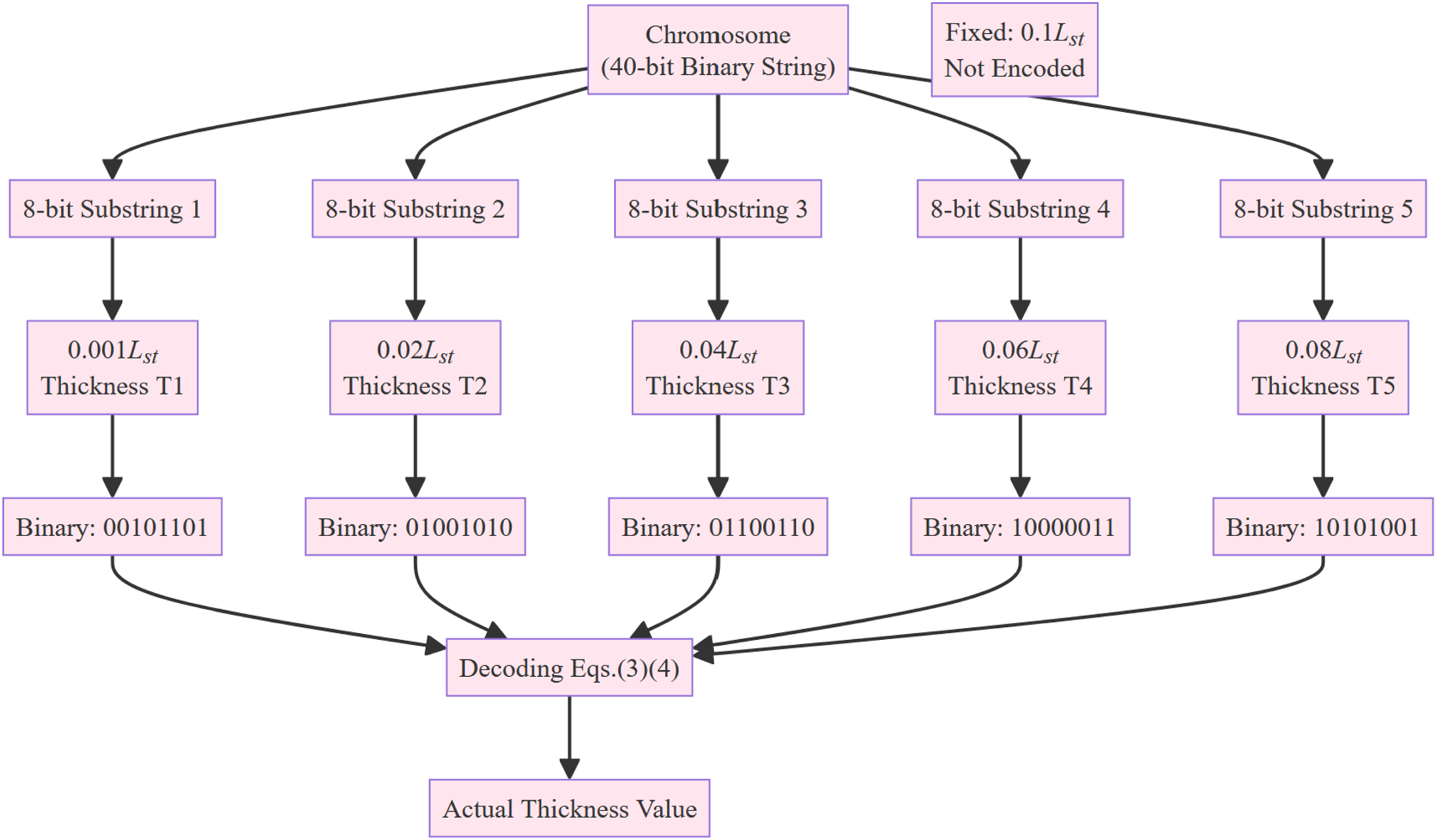

A small initial population of 5 individuals (40-bit chromosomes) is randomly generated to balance computational cost (each individual requires a steady CFD simulation) and optimization efficiency. The iterative GA loop proceeds with three sequential core operations:

Selection/Elimination (100% probability): The fittest individual (highest target function value $F_{tar}$ ) is retained and copied to the next generation, while the worst-performing individual is eliminated to preserve high-quality solutions.

Crossover (60% probability): Random pairs of parent chromosomes exchange segments of their binary substrings at random crossover points, generating offspring chromosomes with combined genetic information to expand the solution space.

Mutation (10% probability): A single bit in the binary chromosome is randomly flipped (0 ↔ 1) at low frequency, introducing minor genetic variations to avoid premature convergence and enhance local search capability.

The GA runs for 100 iterations, and the convergence history (Figure 8) verifies that this setup achieves stable optimization. Although the small population size limits genetic diversity, it represents a practical compromise between computational feasibility and solution accuracy for CFD-based hydrofoil optimization. Future work will explore larger population sizes and adaptive genetic operators to further improve global search performance.

The optimization algorithm is implemented through an in-house C-language program developed by the authors. The program is coupled with the ANSYS CFX solver to establish an automated CFD–GA optimization framework. During the optimization process, the geometric parameters generated by the genetic algorithm are automatically transferred to the CFD solver for flow-field evaluation, and the calculated objective function values are subsequently returned to the optimization program for the next evolutionary iteration. This coupled framework enables efficient iterative evaluation of hydrofoil geometries under multiple incidence-angle conditions.

3.3.2. CFD setup

CFD is used as the solver to evaluate the flow field of individuals. In this study, steady-state Reynolds-averaged Navier–Stokes (RANS) simulations with a single-phase flow assumption are employed to evaluate the cavitation inception characteristics of the hydrofoil. The cavitation tendency is approximated through the minimum pressure coefficient distribution on the hydrofoil surface. This simplified approach is mainly adopted to improve computational efficiency during the optimization process, since each optimization iteration requires repeated CFD evaluations for different hydrofoil geometries and incidence angles.

The present method is effective for rapid optimization and comparative analysis of pressure distribution characteristics. However, it does not capture transient cavitation evolution, vapor–liquid interaction, cavitation bubble collapse, or other unsteady multiphase flow effects associated with cavitation dynamics. More advanced approaches, such as homogeneous mixture models and cavitation transport models, are capable of providing more accurate cavitation predictions but require significantly higher computational cost.

The study reported by Brazhenko and Tarasenko³⁴ is introduced for comparison. In their work, a quasi-steady-state homogeneous mixture model combined with cavitation modeling was employed to reproduce cavitating flow structures and pressure distributions with good agreement to experimental measurements. The study demonstrated that quasi-steady-state numerical models can reliably predict the time-averaged structure of cavitating flows.Compared with such advanced multiphase cavitation models, the present approach focuses more on establishing an efficient optimization framework for leading-edge geometry design under multiple operating conditions.

SST k-ω turbulence model^35,36 is used to close the RANS equation. To close the Reynolds-averaged Navier–Stokes (RANS) equations, the Shear Stress Transport (SST) k–ω turbulence model proposed by Menter is employed in the present study. The SST k–ω model combines the advantages of the standard k–ω model in the near-wall region and the k–ε model in the free-stream region, making it suitable for predicting adverse pressure gradients and flow separation phenomena associated with cavitation inception.The transport equations for the turbulent kinetic energy k and the specific dissipation rate ω are expressed as follows:

\frac{\partial (ρ k)}{\partial t} + \frac{\partial (ρ u_{j} k)}{\partial x_{j}} = P_{k} - β^{*} ρ k ω + \frac{\partial}{\partial x_{j}} [(μ + σ_{k} μ_{t}) \frac{\partial k}{\partial x_{j}}]

(5)

\frac{\partial (ρ ω)}{\partial t} + \frac{\partial (ρ u_{j} ω)}{\partial x_{j}} = α \frac{ω}{k} P_{k} - β ρ ω^{2} + \frac{\partial}{\partial x_{j}} [(μ + σ_{ω} μ_{t}) \frac{\partial ω}{\partial x_{j}}] + 2 (1 - F_{1}) ρ σ_{ω 2} \frac{1}{ω} \frac{\partial k}{\partial x_{j}} \frac{\partial ω}{\partial x_{j}}

(6)

where ρ is the fluid density, uj represents the velocity component in the j direction, k is the turbulent kinetic energy, ω is the specific dissipation rate, μ is the molecular dynamic viscosity, and μt denotes the turbulent eddy viscosity. Pk represents the turbulence production term. The model constants α, β, β*, σk, and σω are empirical coefficients of the SST k–ω model, while F1 is the blending function used to combine the k–ω and k–ε formulations in different flow regions.

The turbulent eddy viscosity is calculated as:

μ_{t} = \frac{ρ a_{1} k}{\max (a_{1} ω, S F_{2})}

(7)

The SST k–ω turbulence model has been widely validated in turbomachinery simulations and is considered suitable for predicting the leading-edge flow separation and pressure distribution associated with cavitation inception phenomena.

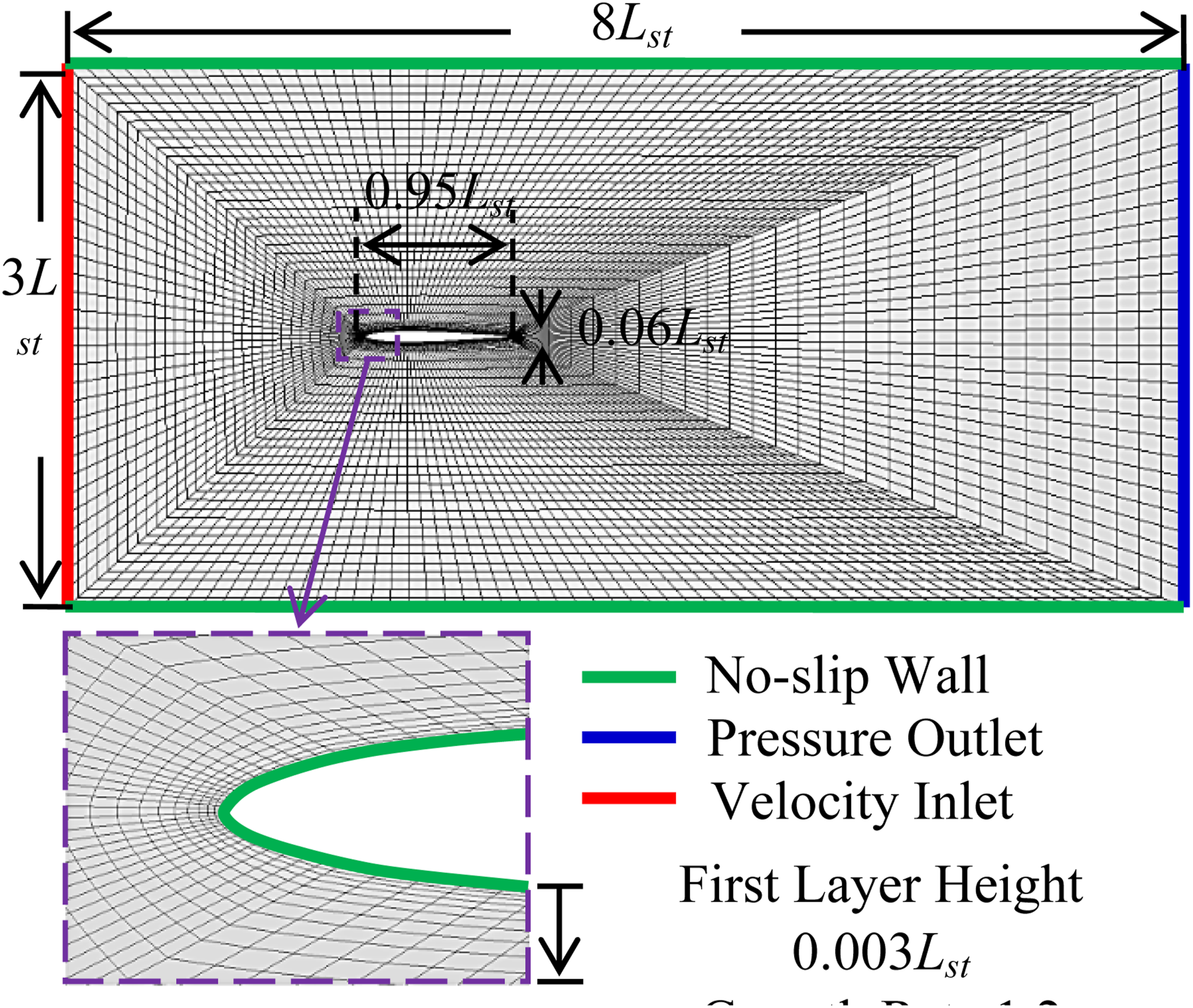
The flow domain, mesh and boundary conditions are illustrated in Figure 5. A simplified two-dimensional domain is used without spanwise L_sp direction. As previouly shown in Figure 3, the length of hydrofoil is L_foil=0.95L_st, the maximum thickness is T_Bmax=0.06L_st.Thus, the outside field size is set to 3L_st×8L_st. No-slip wall conditions are given on the foil surface, top-boundary and bottom-boundary. The pressure outlet condition is set on the downstream-boundary. The velocity inlet condition is set on the upstream-boundary with a uniform distribution of velocity V_in. The Reynolds number in this case is expressed as:

R e = V_{i n} L_{f o i l} / υ

(8)

where υ is the kinematic viscosity of 20°C liquid water. In this case, Re varies from 7.9 × 10⁵ to 14.8 × 10⁵.

Figure 5.

Flow domain, mesh and boundary conditions for CFD.

To make a balance between time and accuracy, a mesh independence study was conducted to evaluate the influence of mesh density on the numerical results. Six different mesh densities ranging from approximately 10 thousand to 34 thousand nodes were tested. The minimum pressure coefficient Cpmin was selected as the monitoring parameter because it is directly related to cavitation inception characteristics.The calculated Cpmin values under different mesh densities are shown in Figure 6. It can be observed that the numerical results change noticeably when the mesh density is relatively coarse. However, after the mesh node number exceeds approximately 23 thousand, the variation of Cpmin becomes very small. The relative variation between the last three mesh cases is within 0.2%, indicating that the numerical results are sufficiently mesh independent.Considering both computational accuracy and efficiency, the mesh containing approximately 23 thousand nodes is selected for the subsequent numerical simulations (Table 2).

Figure 6.

Mesh independence analysis based on minimum pressure coefficient Cpmin.

Table 2.

Comparison of the minimum pressure coefficient Cpmin under different mesh densities.

Mesh node number (×10³)	$C_{p m i n}$
9.992	-2.563
14.986	-2.515
19.622	-2.51
23.058	-2.453
27.808	-2.457
33.666	-2.456

The first layer off-wall is 0.003L_st for applying wall functions, the growth rate of element height off-wall is 1.2. The solved y⁺ on foil surface is 18∼67 under all the solved conditions which meets the wall function requirements.^37,38

The CFD simulations in the present study are conducted using the commercial software ANSYS CFX. The flow field around the hydrofoil is solved based on the Reynolds-averaged Navier–Stokes (RANS) equations together with the SST k–ω turbulence model. ANSYS CFX is employed due to its robustness and reliability in turbomachinery flow simulations involving adverse pressure gradients and flow separation phenomena.

3.3.3. Optimization target function

In this case, incidence angle α=0 degree, α=3 degrees and α=5 degrees are considered. α=0 degree represents the design load condition, α=3 degrees and 5 degrees represent the off-design conditions. The optimization target function, also known as the GA’s fitness function, F_tar is a weighted value of pressure coefficient C_p for α=0, 3 and 5 degrees:

C_{p} = 2 (p - p_{i n}) / ρ V_{i n}^{2}

(9)

F_{t a r} = \sum_{α = 0, 3, 5} w_{α} C_{p α}

(10)

where p is the pressure, p_in is the average pressure value on inlet boundary, ρ is the density, w_α is the weight value for α, C_pα is the minimum C_p value for α. w_α are valued as w₀=0.1, w₃=0.3 and w₅=0.6. It means that off-design conditions are concerned more especially at α=5 degrees. The weight w₀ and w₃ are used for keeping balance of the conditions. Above all, the higher F_tar is, the better incipient cavitation performance is.

The weighting factors (w0 = 0.1, w3 = 0.3, and w5 = 0.6) are selected based on the engineering background of pump cavitation suppression design. In practical pump operation, larger incidence angles usually correspond to off-design operating conditions, such as excessive flow rate or low flow rate conditions. Under these operating conditions, flow separation and low-pressure regions are more likely to develop on the suction or pressure surfaces of the blade, resulting in more severe cavitation problems.

Therefore, larger weighting factors are assigned to higher incidence angles in order to emphasize the anti-cavitation performance under off-design conditions. In contrast, the zero-incidence-angle condition approximately represents the design operating condition of the pump, where the incoming flow direction is more consistent with the blade geometry, leading to smoother flow behavior and lower cavitation risk. Nevertheless, the design condition still needs to be considered during optimization, and thus a smaller but non-zero weighting factor is assigned.

Since the present study mainly focuses on the feasibility and fundamental methodology of cavitation-oriented hydrofoil optimization, a systematic sensitivity analysis of different weighting factor combinations has not yet been carried out. Such investigations will be performed in future studies involving practical pump blade optimization cases with stronger engineering relevance. The flow chart of the entire loop of GA optimization is shown in Figure 7.

Figure 7.

Flow chart of the entire loop of GA optimization.

3.4. Execution and result

3.4.1. Execution process

The optimization is executed for 100 iterations and manually checked. As shown in Figure 8, the highest F_tar value increases from -3.22 to -2.66, the lowest-highest difference of F_tar diminishes from 1.08 to 0.03. In the last 10 generations, the residual of the highest F_tar is less than 0.32%, the residual of the lowest F_tar is less than 2.89%. Generally, both the highest F_tar and the lowest-highest difference of F_tar turn into slightly varying. This optimization is manually regarded as converged after 100 generations.

Figure 8.

Execution process of optimization.

3.4.2. Profiles comparison

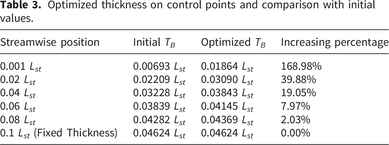
The highest F_tar individual in the last generation is determined as the optimized profile. Figure 9 comparatively shows the initial profile and the optimized profile. The thickness comparisons between two profiles are also listed in Table 3. Result shows that T_B overall increases on all the control points. The closer point to leading edge, the higher increasing is. As shown in Figure 9, the hydrofoil profile changes from “sharp” to “blunt”.

Figure 9.

Initial profile and optimized profile.

Table 3.

Optimized thickness on control points and comparison with initial values.

Streamwise position	Initial T_B	Optimized T_B	Increasing percentage
0.001 L_st	0.00693 L_st	0.01864 L_st	168.98%
0.02 L_st	0.02209 L_st	0.03090 L_st	39.88%
0.04 L_st	0.03228 L_st	0.03843 L_st	19.05%
0.06 L_st	0.03839 L_st	0.04145 L_st	7.97%
0.08 L_st	0.04282 L_st	0.04369 L_st	2.03%
0.1 L_st (Fixed Thickness)	0.04624 L_st	0.04624 L_st	0.00%

4. Verification

4.1. Facilities and methods

The verification experiments are conducted in a cavitation tunnel.In the cavitation tunnel experiments, the flow velocity is measured using an electromagnetic flowmeter and converted into velocity based on the test-section cross-sectional area, with an accuracy of ±0.5%. Pressure data are acquired using a high-precision pressure transducer with a measurement range of 0–2 MPa and an accuracy of ±0.02% full scale (FS). Cavitation visualization is conducted using a high-speed camera operating at 10,000 fps with a resolution of 1280 × 800 pixels. In addition, a National Instruments (NI) data acquisition (DAQ) system with a sampling frequency of 100 kHz and a 16-bit resolution is employed to synchronously acquire flow velocity, pressure, and image trigger signals, ensuring the synchronization and accuracy of the experimental measurements. The test section, which is shown in Figure 10, is made by stainless steel frame with transparent plexiglass walls. The size of the test section is 150mm×150mm×750mm as illustrated. The visualization of cavitation is based on high-speed photographing. The camera is set on the top view focusing on the upper surface of hydrofoil. Both the initial and optimized symmetric hydrofoils are tested within α=0 to 6 degrees. Upstream reference velocity V_∞ and pressure p_∞ are controllable to specify the cavitation level. Non-dimensional cavitation coefficient C_σ is used:

C_{σ} = 2 (p_{\infty} - p_{v}) / ρ V_{\infty}^{2}

(11)

where p_v is the saturation pressure. In this test, p_∞ varies from vacuum to 1.9 Atm, Re varies from 7.9 × 10⁵ to 14.8 × 10⁵. The cavitation level varies from cavitation-free to large scale in different incidence angle cases.

Figure 10.

Test section and the test method.

The two hydrofoils are made by stainless steel as shown in Figure 11. The spanwise length L_sp is 150 mm, streamwise foil length Lf_oil=0.95L_st is 95 mm, maximum thickness T_Bmax is 6 mm. The hydrofoil surface is well-polished where arithmetic average roughness R_a is 0.4 μm. Based on boundary layer study and considering the fully-developed turbulent in pump impeller,³⁹ a micro roughness layer are put on the hydrofoil leading edge. As shown in Figure 10, the roughness layer is made by 60-μm-diameter sand particles which are uniformly distributed on the front 4 mm part of foil surface.

Figure 11.

Hydrofoils manufactured for cavitation test.

4.2. Results

4.2.1. Incipient cavitation

The incipient cavitation coefficient C_σi is the C_σ value once the first bubble is visibly observed on the hydrofoil surface. The C_σ values of initial foil and optimized foil at α=0, 1, 2, 3, 4, 5 and 6 degrees are plotted in Figure 12. According to the comparison, the initial foil has lower C_σi at α=0, 1 and 2 degrees, the optimized foil has lower C_σi at α= 4, 5 and 6 degrees. The C_σi curves intersect around α=3 degrees. A lower C_σi value means that the cavitation incepts later. Therefore, the comparative result of C_σi shows that the optimized foil has an improved anti-incipient-cavitation performance from α=4 to 6 degrees. For pumps, the optimization is successful in delaying the incipient cavitation under “off-design conditions”.

Figure 12.

Incipient cavitation coefficient C_σi at α=0 to 6 degrees.

4.2.2. Visualization of cavitation

Figure 13 shows the visualized comparison of both incipient and developed cavitation between initial foil and optimized foil. As an example, the conditions α=0, 3 and 5 degrees are discussed.

Figure 13.

Comparison of cavitation status between initial and optimized hydrofoils. (a) α=0 degree; V_∞=14.8 m/s, (b) α=3 degrees; V_∞=11.2 m/s, (c) α=5 degrees; V_∞=9.6 m/s.

Figure 13(a) is the photographs at α=0 degree, V_∞=14.8 m/s. Under this condition, C_σi of the initial foil is lower than that of the optimized foil. When C_σ is reduced to 0.73, cavitation incepts on the optimized foil along the leading edge. However, the flow field around the initial foil is cavitation-free. When C_σ is reduced to 0.55, few bubbles incept on the initial foil. At the same time, the maximum cavity length L_cav on the optimized foil becomes approximately 7 mm. When C_σ is reduced to 0.34, L_cav is approximately 10 mm on the initial foil and approximately 34 mm on the optimized foil. For the case α=0 degree, cavitation on optimized foil incepts earlier and performs larger-scale in the same C_σ case.

Figure 13(b) is the photographs at α=3 degree, V_∞=11.2 m/s. Under this condition, C_σi values are similar between initial foil case and optimized foil case. When C_σ is reduced to 2.0, cavitation incepts on leading edge at the same time in initial foil case and optimized foil case. When C_σ is reduced to 1.3, L_cav is approximately 7 mm on the initial foil and approximately 9 mm on the optimized foil. When C_σ is reduced to 0.9, L_cav is approximately 21 mm on the initial foil and approximately 24 mm on the optimized foil. The cavitation scale on initial foil is only slightly smaller than that on optimized foil. For the case α=3 degrees, the cavitation behavior on initial foil and optimized foil are quite similar.

Figure 13(c) is the photographs at α=5 degree, V_∞=9.6 m/s. Under this condition, C_σi of the initial foil is higher than that of the optimized foil. When C_σ is reduced to 3.0, cavitation incepts on the initial foil along the leading edge. The flow field around the optimized foil is cavitation-free. When C_σ is reduced to 2.4, few detached bubbles incept on the optimized foil. At the same time, L_cav is approximately 7 mm on the initial foil. When C_σ is reduced to 1.8, L_cav is approximately 16 mm on the initial foil and approximately 8 mm on the optimized foil. For the case α=5 degrees, incipient cavitation on optimized foil is delayed, the cavitation scale on optimized foil is also smaller than on initial foil in the same C_σ case.

4.2.3. Developed cavitation

A general comparison of cavitation scale between initial foil and optimized foil is shown in Figure 14.The cavity length during cavitation development varies continuously with time due to the inherently unsteady nature of cavitation phenomena. Therefore, the cavity length values presented in Figure 14 represent time-averaged cavity lengths obtained during the visualization process rather than instantaneous measurements.To improve the reliability of the experimental analysis, vertical error bars are introduced in Figure 14 to indicate the fluctuation range of the measured cavity length. The uncertainty levels are estimated according to different incidence angles. Relative uncertainties of 5%, 7.5%, 8%, 9.5%, 10.5%, 11%, and 13% are assigned for incidence angles of 0°, 1°, 2°, 3°, 4°, 5°, and 6°, respectively.The increasing uncertainty with incidence angle mainly results from the stronger instability, cavity shedding behavior, and oscillation intensity of cavitation structures under off-design operating conditions.

Figure 14.

Maximum cavity length L_cav covering on hydrofoil surface.

The relationship between C_σ and L_cav are studied for α=0 to 6 degrees. The rightmost point in each α-based data set represents the incipient cavitation coefficient C_σi. When α<3 degrees, C_σi on initial foil is smaller than on optimized foil, L_cav on initial foil is also smaller than on optimized foil at the same C_σ. Conversely, when α>3 degrees, C_σi on optimized foil is smaller than on initial foil, L_cav on optimized foil is also smaller than on initial foil at the same C_σ. For pumps, the optimized profile has not only a better anti-incipient-cavitation performance but also a better prevention of cavitation development for “off-design conditions”.

4.3. Analysis of hydrofoil

To analyze the geometry and pressure distributions on hydrofoil, a X-Y coordinate based on T_B direction, L_st direction and incidence angle α is established. As shown in Figure 15, X is along the incoming flow and Y is perpendicular to X. To understand why cavitation is different between the initial and the optimized foils, four important parameters are studied in Figure 16. Firstly, the pressure coefficient C_p is studied. C_p and incipient cavitation strongly correlate to each other. “Incipient cavitation” is the moment that p_min≈p_v. Considering both equations (6) and (8), there are relationships that p_in=p_∞ and V_in=V_∞. Therefore, the incipient cavitation coefficient C_σi and the minimum pressure coefficient C_pmin have following relationships:

C_{σ i} = 2 (p_{\infty} - p_{v}) / ρ V_{\infty}^{2} \approx - 2 (p_{\min} - p_{\infty}) / ρ V_{\infty}^{2} = - C_{p m i n}

(12)

Figure 15.

Coordinate X-Y using for analysis of hydrofoil.

Figure 16.

Analysis of the parameters of hydrofoil; SS: Suction Surface, PS: Pressure Surface; d(Y/T_Bmax)/d(X/L_st) and d(C_p)/d(X/L_st) are absolute value.

Secondly, the gradient of C_p along X direction, dC_p/d(X/L_foil), is also studied where non-dimensional X/L_foil is used. Thirdly, the geometry variation Y/T_Bmax is studied because the flow regime and pressure distribution is strongly influenced by foil geometry. At last, the geometric gradient along X direction, d(Y/T_Bmax)/d(X/L_foil), is studied. As shown in Figure 16, the logarithmic scale is used for the horizontal axis X/L_st to emphasize the differences around leading edge. The vertical axis of dC_p/d(X/L_foil) and d(Y/T_Bmax)/d(X/L_foil) are also logarithmic distributed.

At α=0 degree, Y/T_Bmax of optimized foil is larger than initial foil when 0≤X/L_foil≤0.073. The d(Y/T_Bmax)/d(X/L_foil) of optimized foil is also larger than initial foil when 0≤X/L_foil≤0.014. The larger value and faster increasing rate of Y/T_Bmax causes a larger dC_p/d(X/L_foil) on the optimized foil surface when 0≤X/L_foil≤0.1. Thus, the value of C_p diminishes to C_pmin=-0.95 on optimized foil and C_pmin=-0.37 on initial foil. The lower C_p value on optimized foil causes an earlier cavitation occurrence than on initial foil at α=0 degree.

At α=3 degrees, d(Y/T_Bmax)/d(X/L_foil) on optimized foil is larger than initial foil when 0≤X/L_foil≤0.01. However, d(Y/T_Bmax)/d(X/L_foil) on optimized foil becomes smaller than initial foil when 0.01≤X/L_st≤0.1. The different d(Y/T_Bmax)/d(X/L_foil) variation between two foils causes the different C_p distributions. On the initial foil, C_p reduces to C_pmin=-2.16 when 0≤X/L_foil≤0.002. On the optimized foil, C_p reduces to C_pmin=-2.29 when 0≤X/L_foil≤0.011. Generally, because of the similar C_pmin value and also similar dC_p/d(X/L_foil) distributions, initial foil and optimized foil have similar occurrence and development of cavitation at α=3 degrees.

At α=5 degrees, d(Y/T_Bmax)/d(X/L_foil) on optimized foil is slightly larger than on initial foil when 0≤X/L_foil≤0.01. Then, d(Y/T_Bmax)/d(X/L_foil) on initial foil becomes much larger than on optimized foil when 0.01≤X/L_foil≤0.1. Consequently, on the initial foil, C_p reduces to -3.89 at 0≤X/L_foil≤0.0009. On the optimized foil, C_p reduces to -3.01 at 0≤X/L_foil≤0.007. Moreover, the dC_p/d(X/L_foil) value on optimized foil is also smaller than on initial foil when 0≤X/L_foil≤0.1. Thus, both the incipient cavitation is delayed and the developed scale of cavitation are diminished on the optimized foil at α=5 degrees.

4.4. Lift/drag force

The lift and drag force are also important performance for hydrofoil and pump blade. Figure 17 comparatively shows the ratio between lift and drag force, F_L/F_D, on initial foil and optimized foil at α=0 to 6 degrees. After optimization, there are slight F_L/F_D declines which is less than 5%. The change of F_L/F_D should be discussed in the actual pump design cases. Centrifugal or mixed flow impellers work on liquid by rotating centrifugal force. A slight change of leading edge thickness would not obviously change the performance such as head and efficiency. For axial impellers, lift and drag force is the main working force to pressurize the liquid. Thus, the profile shape of axial impeller blade is much more sensitive than that of centrifugal and mixed-flow impellers. When applying the leading edge thickness optimization to axial impellers, the lift/drag force ratio should be seriously checked in case of the performance changes such as efficiency decline, best-efficient-point shift, insufficient head, over-loading of power, etc. The proposed optimization method demonstrates effectiveness for the present hydrofoil case and shows potential for leading-edge shape design in most pump blade applications. In the present study, the hydrofoil is employed as a simplified model of pump blade sections to investigate the fundamental cavitation suppression mechanism. Therefore, the proposed method is expected to provide useful guidance for anti-cavitation design of pump blades, especially under off-design operating conditions commonly encountered in engineering applications.

Figure 17.

Lift/drag force ratio at α=0 to 6 degrees.

5. Conclusions

To improve the anti-incipient-cavitation performance of pump blade profile especially for off-design conditions, optimizations are conducted in this study based on a NACA0006 hydrofoil case study. Conclusions are drawn as follows:

1. Cavitation usually incepts near the leading edge of hydrofoil or pump blade profile. In traditional pump blade profile designs, it is very difficult to have a better anti-incipient-cavitation performance. In this study, an optimization strategy combining GA and CFD solver is used for leading edge thickness modification. To delay the incipient cavitation especially under high incidence angle which represents the off-design conditions, weighted target function is used in this study. The optimized profile, which has a blunter and thicker leading edge shape than initial profile, is found after an evolutional targeted global search. The optimization process is also time-saving by using a simplified 2D flow domain and single-phase flow. Generally, the optimization method for incipient cavitation in this study is effective and easy-executing.

2. Results of the hydrofoil case study show that the foil profile shape strongly influences the incipient and developed cavitation. For the same profile, its geometry along flow direction changes a lot because of the incidence angle variation. Moreover, the variations of geometry and geometric gradient affect the flow regime. Consequently, the different flow regimes cause different distributions of pressure and pressure gradient. The optimized profile, whose leading edge is blunter and thicker than initial profile, got a smaller pressure gradient at high incidence angles that α=4, 5 and 6 degrees. The minimum pressure coefficient on optimized foil increases due to this change. Finally, the incipient cavitation is effectively delayed. The developed cavitation scale on optimized foil is also smaller than initial foil in the same C_σ case.

Above all, this optimization method supplies the pump designs to have a better anti-cavitation performance under off-design conditions and even widen the cavitation-free operation range.

Despite the demonstrated effectiveness, several limitations should be noted. The study is based on a simplified hydrofoil model and a steady single-phase CFD approach. The influence of parameterization strategy, weighting factors, and optimization settings has not been fully explored. Future work will focus on extending the method to three-dimensional blade geometries, incorporating multiphase cavitation models, and performing sensitivity and uncertainty analyses.

Footnotes

Acknowledgements

The authors would like to acknowledge the financial support by National Natural Science Foundation of China (No. U22A20238).

ORCID iDs

Xinyi Xie

Ran Tao

CRediT authorship contribution statement

Xinyi Xie: Writing - original draft, Investigation, MethodologySoftware, Validation, Experimental investigation.

Ran Tao: Writing - review & editing, Supervision, Resources, Project administration.

Funding

The authors disclosed receipt of the following financial support for the research, authorship, and/or publication of this article: This work was supported by the National Natural Science Foundation of China (No. U22A20238).

Declaration of conflicting interests

The authors declared no potential conflicts of interest with respect to the research, authorship, and/or publication of this article.

Data Availability Statement

The data that has been used is confidential.*

Appendix

References

Alavi

Ghasemnezhad

Sangtarash

, et al. Passive cavitation mitigation on hydrofoils via porous media: A comparative study of LES and RANS models. OCEAN ENGINEERING 2025; 341: 122756. https://doi.org/10.1016/j.oceaneng.2025.122756

Chen

, et al. Research on the effects of different blade leading-edge geometries on the internal and external characteristics of centrifugal pumps. OCEAN ENGINEERING 2024; 309: 118371.

Huo

Zha

. Influence of blade leading-edge form on the performance and internal flow pattern of a mixed-flow pump. FRONTIERS IN ENERGY RESEARCH 2023; 11: 1292387. https://doi.org/10.3389/fenrg.2023.1292387

Kumar

Kadivar

El Moctar

. Experimental study of cavitation control on a hydrofoil with bio-inspired riblets using proper orthogonal decomposition. OCEAN ENGINEERING 2025; 334: 121500. https://doi.org/10.1016/j.oceaneng.2025.121500

Qian

Zhang

Xue

. Numerical Study of Mitigating Cloud Cavitation Shedding Using Biomimetic Protuberant Stripes. JOURNAL OF FLUIDS ENGINEERING-TRANSACTIONS OF THE ASME 2022; 144(9): 091201. https://doi.org/10.1115/1.4053680

Sun

Song

Sun

, et al. Cavitation Suppression and Design Optimization in a Cryogenic Liquid Turbine Expander Based on Thermodynamic Cavitation and Entropy Production Analysis. JOURNAL OF FLUIDS ENGINEERING-TRANSACTIONS OF THE ASME 2023; 145(1): 011201. https://doi.org/10.1115/1.4055179

Tchada

Tchoumboue

Mesquita

, et al. Enhancing Pump as Turbine (PAT) performances: A numerical investigation into the impact of impeller leading edge rounding. HELIYON 2024; 10(15): e34663. https://doi.org/10.1016/j.heliyon.2024.e34663

Zhang

Zheng

Shao

, et al. Multiscale modeling of propeller cavitation flows in open water. JOURNAL OF HYDRODYNAMICS 2025; 37(3): 478–488. https://doi.org/10.1007/s42241-025-0036-z

Brennen

. Cavitation and bubble dynamics. Cambridge University Press, 2013.

10.

Rus

Dular

Širok

, et al. An investigation of the relationship between acoustic emission, vibration, noise, and cavitation structures on a Kaplan turbine. Journal of Fluids Engineering 2007; 129(9): 1112–1122. https://doi.org/10.1115/1.2754313

11.

Liao

Qiu

, et al. Research progresses on cavitation induced noise of centrifugal pump. Journal of Ship Mechanics 2022; 26(5): 761–773.

12.

Çelik

Usta

Öksüz

, et al. Experimental investigation of leading-edge tubercle and surface corrugation effects on cavitation and noise in partially cavitating twisted hydrofoils. OCEAN ENGINEERING 2025; 324: 120646. https://doi.org/10.1016/j.oceaneng.2025.120646

13.

Cheng

Shao

Fan

. Impacts of Cavitation on Flow Field Distributions and Pump Stability in Cryogenic Pumps. JOURNAL OF LOW TEMPERATURE PHYSICS 2023; 211(1-2): 86–107. https://doi.org/10.1007/s10909-023-02944-8

14.

Yang

Xiao

Wang

, et al. Influence of splitter blades on the cavitation performance of a double suction centrifugal pump. Advances in Mechanical Engineering 2014; 6: 963197. https://doi.org/10.1155/2014/963197

15.

Yao

Xiao

Wang

, et al. Numerical Investigation of Cavitation Improvement for a Francis Turbine. In: Journal of Physics: Conference Series. IOP Publishing, 2015, Vol. 656, No. 1, p. 012075. https://doi.org/10.1088/1742-6596/656/1/012075

16.

Luo

Zhang

Peng

, et al. Effect of impeller inlet geometry on centrifugal pump cavitation performance. Journal of Tsinghua University (Science and Technology) 2008; 5: 018.

17.

Bosioc

Stuparu

Tanasa

, et al. Flat free runner with outer ring for reducing the hydraulic instabilities developed in the discharge cone of a Francis turbine. In: 9TH IAHR MEETING OF THE WORKGROUP ON CAVITATION AND DYNAMIC PROBLEMS IN HYDRAULIC MACHINERY AND SYSTEMS, Timisoara, Romania, October 10-12, 2025, p. 1483.

18.

Motycak

Skotak

Kupcik

(2012). Kaplan turbine tip vortex cavitation–analysis and prevention. In: IOP Conference Series: Earth and Environmental Science. IOP Publishing, Vol. 15, No. 3, p. 032060. https://doi.org/10.1088/1755-1315/15/3/032060

19.

Roussopoulos

Monkewitz

. Measurements of tip vortex characteristics and the effect of an anti-cavitation lip on a model Kaplan turbine blade. Flow, Turbulence and Combustion 2000; 64(2): 119–144. https://doi.org/10.1023/a:1009976411156

20.

Zhu

Xiao

Liu

. Influence of leading-edge cavitation on impeller blade axial force in the pump mode of reversible pump-turbine. RENEWABLE ENERGY 2021; 163: 939–949. https://doi.org/10.1016/j.renene.2020.09.002

21.

Yang

Zhang

Shen

, et al. Investigation on flow instability in the hump region of the large vertical centrifugal pump under cavitation conditions based on proper orthogonal decomposition. PHYSICS OF FLUIDS 2024; 36(11): 115134. https://doi.org/10.1063/5.0236649

22.

Zhang

, et al. Numerical investigation of unsteady leading edge cavitation in a double-suction centrifugal pump. PHYSICS OF FLUIDS 2024; 36(9): 093351.

23.

Balasubramanian

Bradshaw

Sabini

. Influence of impeller leading edge profiles on cavitation and suction performance. In: Proceedings of the 27th International Pump Users Symposium, Houston, Texas, September 2011, pp. 12–15.

24.

Yang

, et al. Bionic leading-edge protuberances and hydrofoil cavitation. PHYSICS OF FLUIDS 2021; 33(9): 093317. https://doi.org/10.1063/5.0069587

25.

Zhou

. Draft head options for pump turbine of pumped storage plant. Mechanical & Electrical Technique of Hydropower Station 2006; 4: 004.

26.

Zhang

Zang

Shi

, et al. Analysis of the Formation Mechanism and Evolution of the Perpendicular Cavitation Vortex of Tip Leakage Flow in an Axial-Flow Pump for Off-Design Conditions. JOURNAL OF MARINE SCIENCE AND ENGINEERING 2021; 9(10): 1045. https://doi.org/10.3390/jmse9101045

27.

Wang

. A method for inverse calculation of the blade S2 stream surface in centrifugal pump and its application. Journal of Hydraulic Engineering 1998; 1: 10–13.

28.

Gülich

. Centrifugal pumps. Springer, 2008.

29.

Neill

Reuben

Sandford

, et al. Detection of incipient cavitation in pumps using acoustic emission. Proceedings of the Institution of Mechanical Engineers, Part E: Journal of process mechanical engineering 1997; 211(4): 267–277. https://doi.org/10.1243/0954408971529737

30.

Mosetti

Poloni

Diviacco

. Optimization of wind turbine positioning in large windfarms by means of a genetic algorithm. Journal of Wind Engineering and Industrial Aerodynamics 1994; 51(1): 105–116. https://doi.org/10.1016/0167-6105(94)90080-9

31.

Horn

Nafpliotis

Goldberg

. A niched Pareto genetic algorithm for multiobjective optimization. In: Evolutionary Computation, 1994. IEEE World Congress on Computational Intelligence. Proceedings of the First IEEE Conference, Orlando, Florida, June 27-29, 1994, pp. 82–87. IEEE.

32.

Nariman-Zadeh

Amanifard

Hajiloo

, et al. Multi-objective pareto optimization of centrifugal pump using genetic algorithms. In: Proceedings of the 11th WSEAS International Conference on Computers, Crete Islands, Greece, July 26-28, 2007, pp. 135–139.

33.

Menter

. Two-equation eddy-viscosity turbulence models for engineering applications. AIAA Journal 1994; 32(8): 1598–1605. https://doi.org/10.2514/3.12149

34.

Brazhenko

Tarasenko

. Investigation of Cavitation Flow Structure in a Small-Scale Throttle Channel Using a Quasi-Steady-State Numerical Model. Aerospace 2026; 13: 83. https://doi.org/10.3390/aerospace13010083

35.

Menter

Kuntz

Langtry

. Ten years of industrial experience with the SST turbulence model. Turbulence, Heat and Mass Transfer 2003; 4(1).

36.

Salim

Cheah

. Wall Y strategy for dealing with wall-bounded turbulent flows. In: Proceedings of the International MultiConference of Engineers and Computer Scientists, Hong Kong, March 18-20, 2009.

37.

Kim

Choudhury

. A near-wall treatment using wall functions sensitized to pressure gradient. Separated and Complex Flows 1995; 1995: 273–280.

38.

Dreyer

Decaix

Münch-Alligné

, et al. Mind the gap: a new insight into the tip leakage vortex using stereo-PIV. Experiments in Fluids 2014; 55(11): 1–13. https://doi.org/10.1007/s00348-014-1849-7

39.

Ausoni

Zobeiri

Avellan

, et al. The effects of a tripped turbulent boundary layer on vortex shedding from a blunt trailing edge hydrofoil. Journal of Fluids Engineering 2012; 134(5): 051207. https://doi.org/10.1115/1.4006700

Optimization of hydrofoil leading-edge geometry for delaying incipient cavitation using a CFD–GA approach

Abstract

Keywords

1. Introduction

2. Solution Strategy

3. Application example - NACA0006 hydrofoil

3.1. Geometry of hydrofoil

3.2. Parameterization

3.3. GA and CFD setup

3.3.1. GA setup

3.3.2. CFD setup

3.3.3. Optimization target function

3.4. Execution and result

3.4.1. Execution process

3.4.2. Profiles comparison

4. Verification

4.1. Facilities and methods

4.2. Results

4.2.1. Incipient cavitation

4.2.2. Visualization of cavitation

4.2.3. Developed cavitation

4.3. Analysis of hydrofoil

4.4. Lift/drag force

5. Conclusions

Footnotes

Acknowledgements

ORCID iDs

CRediT authorship contribution statement

Funding

Declaration of conflicting interests

Data Availability Statement

Appendix

References