Fabric defect detection using adaptive dictionaries

Abstract

In this paper, we present a new fabric defect detection algorithm based on learning an adaptive dictionary. Such a dictionary can efficiently represent columns of normal fabric images using a linear combination of its elements. Benefiting from the fact that defects on a fabric appear to be small in size, a dictionary can be learned directly from a testing image itself instead of a reference, allowing more flexibility to adapt to varying fabric textures. When modeling a test image using the learned dictionary, columns involving anomalies of the test image are likely to have larger reconstruction errors than normal ones. The anomalous regions (defects) can be easily enhanced in the residual image. Then, a simple threshold operation is able to segment the defective pixels from the residual image. To adapt more defects, especially some linear defects, we rotate the test image by a slight degree and re-analyze the rotated image. Compared to the Fourier method, experimental results on 47 real-world test images with defects reveal that our algorithm is able to adapt to varying fabric textures and exhibits more accurate defect detection.

Keywords

Fabric defect detection novelty detection dictionary learning adaptive representation

In the modern textile industry, visual surface inspection of raw woven fabrics plays an important role in quality control of textile products, as defects on the fabric surface can have a great impact on costs and grading of final products. At present, fabric inspection in textile mills is still performed manually by human inspectors, a process which suffers from both low efficiency and high labor intensity and cannot meet the requirement of high-quality mass manufacturing. Application of computer vision and pattern recognition techniques to fabric defect detection can effectively avoid the limitations of employing human inspectors. In recent decades, numerous algorithms based on computer vision have been proposed to address the problem of fabric defect detection; thorough reviews can be found in Kumar and Mahajan et al.^1,2

In general, images of normal woven fabrics are dominated by a texture which always exhibits a high periodicity among sub-patterns, due to the characteristics of the weaving process used in fabric formation. If a defect is present, the local regularity (periodicity) of a fabric will be disrupted, resulting in an imperfection or anomaly against the homogeneous texture. With this observation, to inspect defects with computer vision techniques, a defect in a fabric image is usually defined as any abnormality deriving from the homogeneous texture background. How to describe such anomalies (defects) becomes a baseline for researchers to design detection algorithms. In terms of defect detection strategy, fabric defect detection schemes can be categorized into feature-extraction-based and non-feature-extraction-based. In the first approach, feature extraction is of great importance in fabric detection, which involves extracting efficient textural features in spatial and/or spectral domains that are capable of robustly characterizing background fabric textures and sensitive to the abnormal regions caused by defects. In the spatial domain, some widely used texture features for detecting defects include neighboring information,^3,4 the gray level co-occurrence matrix,⁵ and fractal dimensions;⁶ in the spectral domain, Fourier spectral features,^7, ⁸ wavelet transform coefficients,^9,10 Gabor wavelet features,¹¹ and auto-regressive spectral analysis are used.¹² One of the difficult tasks of the feature extraction approach is to find general features that can guarantee to adapt various types of fabrics and defect, since there is no straightforward way to judge the appropriate features to use. Of the non-feature extraction detection schemes, Gabor filters is considered to be the most successful approach for detecting fabric defects,^13–15 in that it does not need an explicit feature extraction stage but utilizes a set of optimized Gabor filters and segment defects from the filtered images straightforwardly. However, the choice of filter parameters is a quite complicated task, since the detection performance heavily relies on how the filters can match or be tuned to the property of a specific defect, e.g. the scale and orientation of a defect. Although several methods have been developed for optimization of filter banks,^{11,14,16–18} a prior knowledge (e.g. templates or defects) is still required for optimizing filters, e.g. artificial defects were involved in training filters,¹¹ limited defect types were used to optimize filter parameters,¹⁴ and non-defective samples were required to optimize filters using a Gabor wavelet network.^17,18

With the lack of standard benchmarks for comparison of different algorithms, there is only one preliminary comparison among four common texture analysis techniques, such as gray level co-occurrence, normalized cross-correlation, texture blob detection, and spectral methods, suggesting that those methods provide good results on certain types of defects but are poor on others.¹⁹ To our knowledge, the major difficulties making this issue challenging can be concluded to be as follows:

The complexity of fabric textures

Ideally, raw woven fabrics belong to a kind of structural textures composed of repetitive structural patterns determined by weaving structures. However, due to the elasticity of yarns and various weaving settings, real-world fabric images do not exhibit distinct or strong spatial weaving structural units that they should have, but appear to be high stochastic variations on normal fabric surfaces, especially plain fabrics.

The large diversity of defect types

Most of defects arising in the weaving process are caused by unplanned machine malfunctions and others are caused by faulty yarns, resulting in a large number of unpredictable defect types. Since the defects occur in a random way, it is impossible to collect all potential defect types as the negative samples that can be used to optimize parameters or train a classifier to achieve better performance.

To tackle the two aforementioned issues, we propose a new detection algorithm based on learning adaptive dictionaries. The proposed method neither needs any prior information during all detection stages nor relies on extracted features, so that it can avoid all aforementioned limitations of feature extraction schemes. To address problem (a), our algorithm aims to learn a dictionary directly from a test image itself, such that the learned dictionary enables an adaptive representation for each column of the test image using a linear combination of its elements, potentially allowing more flexibility to adapt to varying fabric textures. For problem (b), we focus on identifying defective regions on each column of a test image, whereby the defect detection problem can be converted into finding abnormal changes in a one-dimensional signal (a column) caused by any defects. Since the learned dictionary is tuned to the natural variation of defect-free columns, when modeling the columns containing defects with the learned dictionary, the anomalous regions on those columns cannot be approximated correctly, resulting in a larger reconstruction error. Thus, defective regions can be easily enhanced by calculating the difference between the original column and its approximation.

Related work

In related work, Tsai and Hsieh presented a global approach based on a Fourier image reconstruction scheme to detect defects on oriented textures.²⁰ Tsai and Huang also adopted a Fourier image reconstruction scheme for inspection of defects on random textures.²¹ Taking advantage of the inverse Fourier transform, both of the aforementioned methods attempt to remove the background and preserve defective information by setting the high-energy frequency components to zero in the spectral domain. Since the high-energy frequency components correspond to the background information, performing an inverse Fourier transform after setting them to zero will only restore those regions associating defects. Tsai and Hsiao applied wavelet restoration techniques based on a global image for surface inspection of texture materials.²² The authors decomposed an image into several sub-images using multi-resolution wavelet transforms. By choosing proper sub-images for reconstruction, the defective regions will be enhanced in the reconstructed image, and then binary thresholding is used to segment defects. Sezer et al. have used independent components analysis (ICA) for fabric defect detection.²³ ICA can be viewed as a linear transformation which decomposes input data into a linear combination of basis elements that are statistically independent. The success of the approach relies on the bar or grating cell-like independent components (ICs) extracted from the texture image, which are expected to respond differentially to defective and defect-free regions.

Instead of transforming an image into the spectral domain to perform restoration, our algorithm is able to learn a simple and more explicit dictionary to address this issue. Such a dictionary learned from input data is able to efficiently represent each column of defect-free images as a linear combination of its elements. Benefiting from the fact that defects appear to be small in size, a dictionary can be learned directly from test images (normal or defective images) instead of a reference one. With the learned dictionary, those normal columns can be approximated well, since it captures the key features of normal samples, allowing for their natural variations. On the other hand, columns with anomalies not found in normal fabric samples will have a substantially larger reconstruction error. When approximating all the columns of the test image, the anomalous regions (defects) can be enhanced in the residual image resulting from a subtraction of the original and its approximation. Then, a simple thresholding operation can be utilized to segment the anomalies regions from the residual image. To adapt more defects especially some linear defects, we rotate the testing image by a slight degree and re-analyze the rotated image using the same algorithm implemented on the original image. Then, two detection results from the original image and its rotated version are merged into one as the final output.

The remainder of this paper is organized as follows. A brief introduction to dictionary learning and the fabric defect detection scheme appear in the next section. The experimental results and discussion are presented in the following section. A conclusion follows in the last section.

Dictionary learning and fabric defect detection

In recent years, dictionary learning based on sparse representation has received a great deal of attention, and has been successfully applied to many computer vision problems.^24–26 The success of a sparse representation owes itself to the flexibility of using a learned over-complete dictionary and some signals, such as natural images, which are proved to admit a sparse decomposition in an over-complete dictionary. Despite the advantages of a sparse representation, for defect detection purposes we wish to find such a dictionary that is able to represent normal fabric structures well, but defective structures poorly. In this sense, a sparse representation using an over-complete dictionary is not suitable for fabric defect detection. For our defect detection problem, in this paper we do not adopt an over-complete dictionary to admit sparse representation, but instead learn a small-size dictionary that can represent columns of a fabric image using a linear combination of its elements.

Learning adaptive dictionaries

The goal of linear representation of data is to find a linear combination of a small number of basis vectors (called a dictionary) to approximate a signal with minimal mean squared error. Suppose that there is a m × n data matrix X = [x₁, x₂,…,x_n], x_i∈R ^m that contains n vectors of dimension m in its columns. To create an approximation for every vector x_i in X, we need to find a dictionary D = [d₁, d₂,…,d_k], d_j∈R ^m , each column containing a basis vector, that can represent all x_i in X. The problem of finding such a dictionary can be formulated as follows:
${min}_{D, α} \sum_{i = 1}^{n} | | x_{i} - D α_{i} | |_{2} 2, s . t . \forall j = 1, \dots, k, d_{j}^{T} d_{j} \leq 1$
(1)
where α_i in R ^k is the coefficient vector for x_i in X, and the constraint to d₁,…,d_k is to prevent D from having arbitrarily large values. Equation (1) is not a jointly convex problem, but convex with respect to each of the two variables D and α when the other one is fixed. A simple converging algorithm that attempts to minimize equation (1) iteratively minimizes over one of either D or α_i while keeping the other fixed. To solve equation (1) more efficiently, we use the recently developed algorithm which is based on stochastic approximations and can converge quite rapidly even with large-scale data sets.²⁷

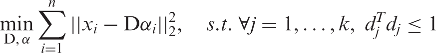
Since image samples used in this paper contain 256 gray levels which can be represented as a matrix whose elements are the gray-level values (intensity) of image pixels, we learn a dictionary D using equation (1) for a fabric image by taking each column of the image as a data vector x_i. When a dictionary is learned from a certain type of fabrics, the learned dictionary will only capture the key structural features of this fabric. Figure 1 presents five dictionary elements learned from a plain and a twill fabric.
Figure 1.
Five dictionary elements learned from a plain and a twill fabric.

Approximation with the learned dictionary

As mentioned above, the dictionary D learned from equation (1) is able to approximate every vector x_i in X. Given a new sample y, one can approximate y with the learned dictionary D by the following equations
$α^{} = {min}_{α} | | y - D α | |_{2} 2 y_{r} = D α^{}$
(2)
where y_r is the approximation to y. Since the learned dictionary D has been tuned to the input data X, it is not difficult to understand if y comes from the same class as x_i in X, the error between y and y_r is likely to be smaller than one from other classes.

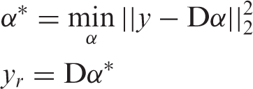
For fabric defect detection, it makes sense to learn a dictionary from a defect-free fabric image to ensure that the learned dictionary can capture the normal structural features of this fabric. However, being vulnerable to skewness or stretch caused by the elasticity of yarns, the dictionary learned from a normal sample or template may not have more advantages than that learned from its defective version. The reason for this is that defects on a fabric generally appear to be small in size compared to the whole image, which has little impact on learning the normal structures. Figure 2 illustrates two approximation examples for a normal fabric and its defective version.
Figure 2.
Two approximation examples for a normal fabric and its defective version.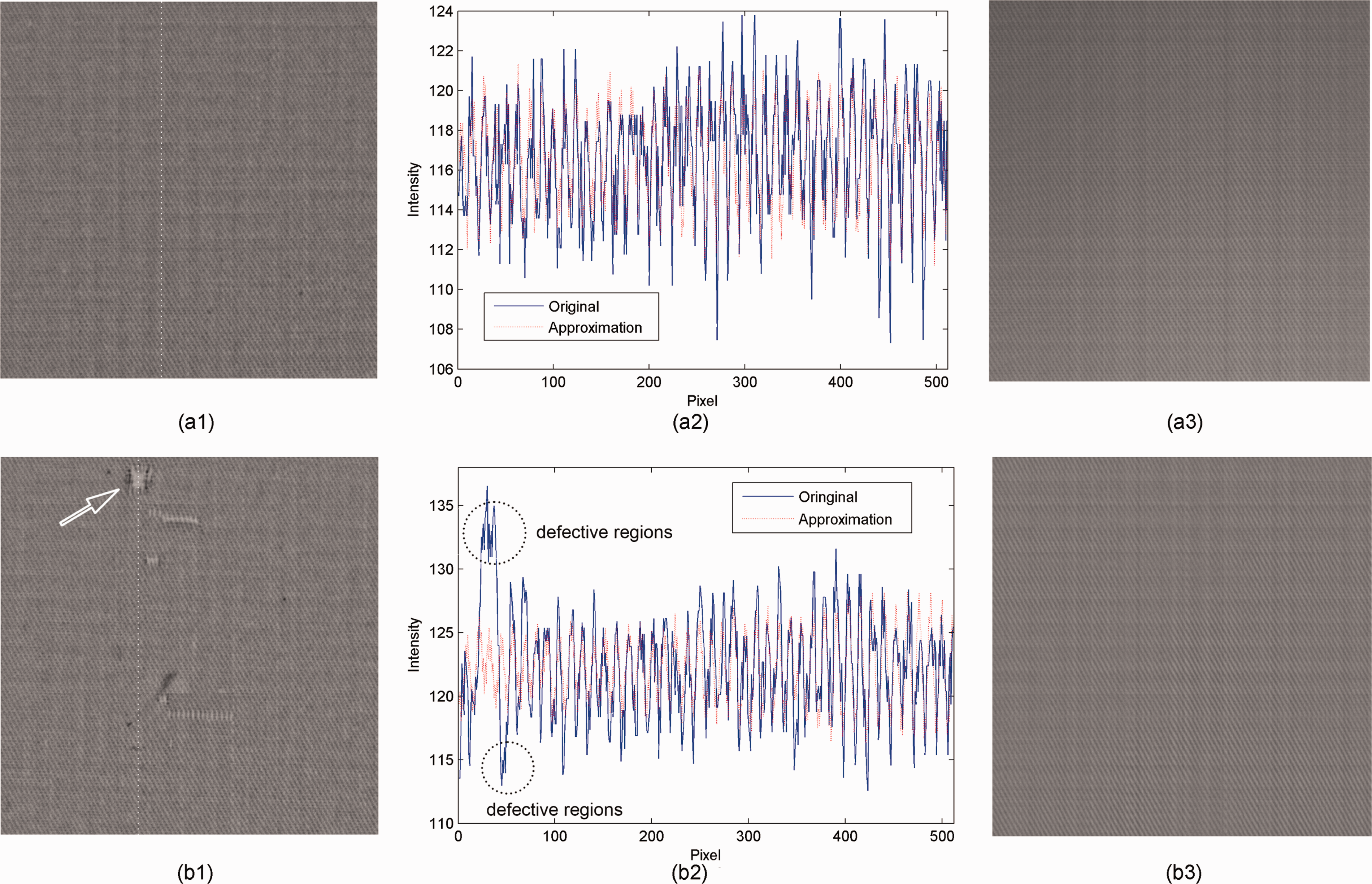

Figure 2(a1) is a defect-free fabric image, which is used to learn a dictionary using equation (1). Figure 2(a2) shows an approximation of the column located at the white dashed line in Figure 2(a1), and Figure 2(a3) shows an overall approximation of Figure 2(a1) after modeling all its columns. Another set of approximation results for the defective version of Figure 2(a1) are presented in Figures 2(b1) to (b3), where Figure 2(b1), the defective version of Figure 2(a1), is used to learn a dictionary, and Figure 2(b2) shows an approximation of the column located at the white dashed line in Figure 2(b1), and Figure 2(b3) shows an overall approximation of Figure 2(b1) after modeling all its columns.

By examining Figure 2(b3), it can be seen that the dictionary learned from the defective version also has the ability to capture its normal background structural features so that it is able to model the normal columns well, while failing to model those anomalous regions caused by defects (see the circles in Figure 2(b2)).

Selection of dictionary size

Before using equation (1) to learn a dictionary from an image sample, the number of elements k (also called dictionary size) of a dictionary needs to be determined beforehand. The parameter k controls the accuracy of reconstruction error, i.e. the larger the k, the smaller the reconstruction error. For defect detection purposes, we wish to find a dictionary that is adequate to model the normal regions well, but not the defective regions. Our experiments show that large dictionary size k is in favor of modeling normal regions, but would increase the possibility of approximating defective regions ‘well’. On the other hand, a large dictionary may introduce some local features (defective regions) as the dictionary is learned from a defective image. Figures 3(a) to (e) demonstrate the absolute value of the residual images under different k. Note that the residual image is obtained by a subtraction of the original image and its approximation after modeling all its columns. It can be found that the total area of defective regions becomes smaller with increasing k, indicating that parts of defective regions are taken as normal regions being approximated, as equation (2) pursues the minimal reconstruction error.
Figure 3.
Absolute value of the residual images under different k values.

To select a proper dictionary size k, we define a cost function based on measuring the residual images. The cost function F(k) is defined as
$F (k) = \frac{σ_{k}}{μ_{k}}$
(3)
where σ_k and μ_k are the standard deviation and mean value calculated from the absolute value of its residual image. In our defect detection problem, the larger σ_k is associated with the better discriminative power (high contrast between defective region and background), and μ_k reflects how well the whole image is approximated.

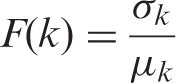
In this paper, we choose the k corresponding to the maximum of F(k) as dictionary size – a k accounts for good approximation and the best discriminative power as well. Figure 3(f) shows an example of cost function F(k) with respect to different k, showing the optimal dictionary size k is 5 (see its residual image in Figure 3(c)). By comparing Figures 3(a) to (e), we find that the area of defective regions begin to decline fast from Figure 3(d) (using k = 6), due to the defective regions being approximated (see the yellow regions on top of Figures 3(c) and (d)). Although Figures 3(a) to (c) (using k = 3, 4, 5) have similar defective area, k = 3, 4 have been proved to be poor in approximating their normal regions, confirming the effectiveness of equation (3) for finding dictionary size.

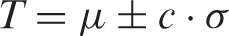
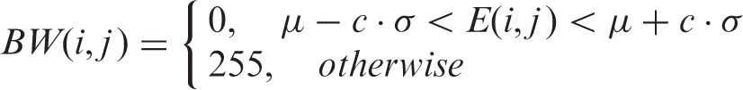
Once dictionary size is determined, a simple thresholding operation can be used to segment the defective regions from the residual image, in which the larger absolute pixel values are doomed to be defects. Since the defective regions are generally small with respect to the entire residual image, a simple density method can be used to estimate the upper and lower boundary of the automatic thresholding value, which is given by the following equation
$T = μ \pm c \cdot σ$
(4)
where μ and σ are the mean and standard deviation of pixel values in the residual image, and c is a pre-selected constant. To determine c statistically, we assume the pixel values in the background region in the residual image follow Gaussian distribution, and the regions having lower probability (large magnitude) are classified as defects. In this work, we set constant c = 2.7, corresponding to 99.31% confidence interval when normalizing the residual image into a standard Gaussian distribution with zero mean and unit variance. The segmentation results is given by a binary image BW
$BW (i, j) = {0, μ - c \cdot σ < E (i, j) < μ + c \cdot σ 255, otherwise$
(5)
where i and j are locations of pixels, and E is the residual image.

Linear defects

In the section on learning adaptive dictionaries, we mentioned the flexibility to learn a dictionary from a test image itself. However, there is a drawback arising from using test images to learn a dictionary. Suppose that there is a defect appearing to be a horizontal line across the whole image (see Figure 4(a1)), such that the anomaly caused by the defect spreads to all columns at the same location. When learning a dictionary from this image, the anomalous regions will be wrongly regarded as parts of the image and be incorporated into the learned dictionary. In this situation, our algorithm turns out to be useless in identifying those types of defects, as the anomalous regions will be well approximated as normal cases. Figure 4(a2) illustrates how our algorithm fails in detecting the linear defect, and can successfully detect the other defective regions that do not share the same anomalies in each column. From Figure 4(a2), it can be seen that only those regions not sharing the same anomalies in each column are detected (see white pixels), while the other defective regions (the white line in the middle of Figure 4(a1)) fail to be detected.
Figure 4.
Effect of a defect appearing as a horizontal line across the whole image.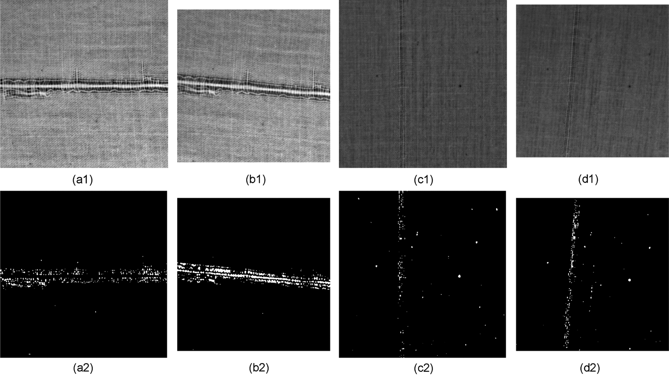

To overcome this problem and make our algorithm adapt to those defects, instead of modifying algorithm, we rotate a testing image by a slight degree (see Figure 4(b1)), such that anomalies on each column will no longer share the same location at each column in the rotated image, ensuring that the anomalous regions does not appear in the learned dictionary. With this understanding, the rotation angle being able to make the linear defective regions in each column have different locations at horizontal direction, will be adequate for learning an expected dictionary that can identify defects as other defects. In other words, for horizontal linear defects, the larger the rotation angle is used, the greater shift will occur, facilitating learning of the right dictionary. Theoretically speaking, rotating at 45° (maximum angle in terms of horizontal direction) is the best for detecting those horizontal defects, and our preliminary results confirmed this argument. But, for practicable application, making a rotation angle of 45° means one will lose half of the image in terms of area, as the rotated image needs to be cropped into a rectangle for analysis. Considering the small scale of linear defects, our experiments showed that 5° of rotation is adequate for detecting linear defects, and that not too much performance is lost compared to that for rotation of 45°.

Benefiting from the repetitive structural patterns of fabrics, the rotated image still holds the repetitive pattern characteristics. When learning a dictionary from the rotated image, the learned dictionary will be tuned to the features of the rotated image, and can be used to detect defects in the rotated image. The successful detection result for a rotated image shown in Figure 4(b2) demonstrates the effectiveness of our algorithm in detecting defects for a rotated image.

Furthermore, our experiment shows that re-analyzing the rotated images also facilitates the identification of some defects appearing as a vertical line across images (see Figure 4(c1)). Such a situation always happens in high-density plain fabrics, since the vertical defects exhibit a high degree of similarity to the background texture. Figures 4(c2) and (d2) show the detection results for Figure 4(c1) and Figure 4(d1). It can be seen that analyzing the rotated version is also favorable for identifying some vertical defects, as it is able to detect more defective regions in its rotated version.

Experiments

Since no standard data set exists and source codes of related approaches are not available for comparison, we demonstrate the efficiency of our algorithm described in the previous section using various types of 52 fabric samples including 47 defective images and five defect-free images. All the test images used in this paper were captured from a production line, and each image has the size 512 × 512 (330 pixels/inch) with 256 gray levels. For the purpose of displaying detection results, we roughly classify all defect types into three categories by their geometry: blocky defects, linear defects, and mixture of both (refer to Figure 5), and the properties of defects such as structure, intensity variation, and defect size are used for discussion.
Figure 5.
Classification of all defect types into three categories by their geometry.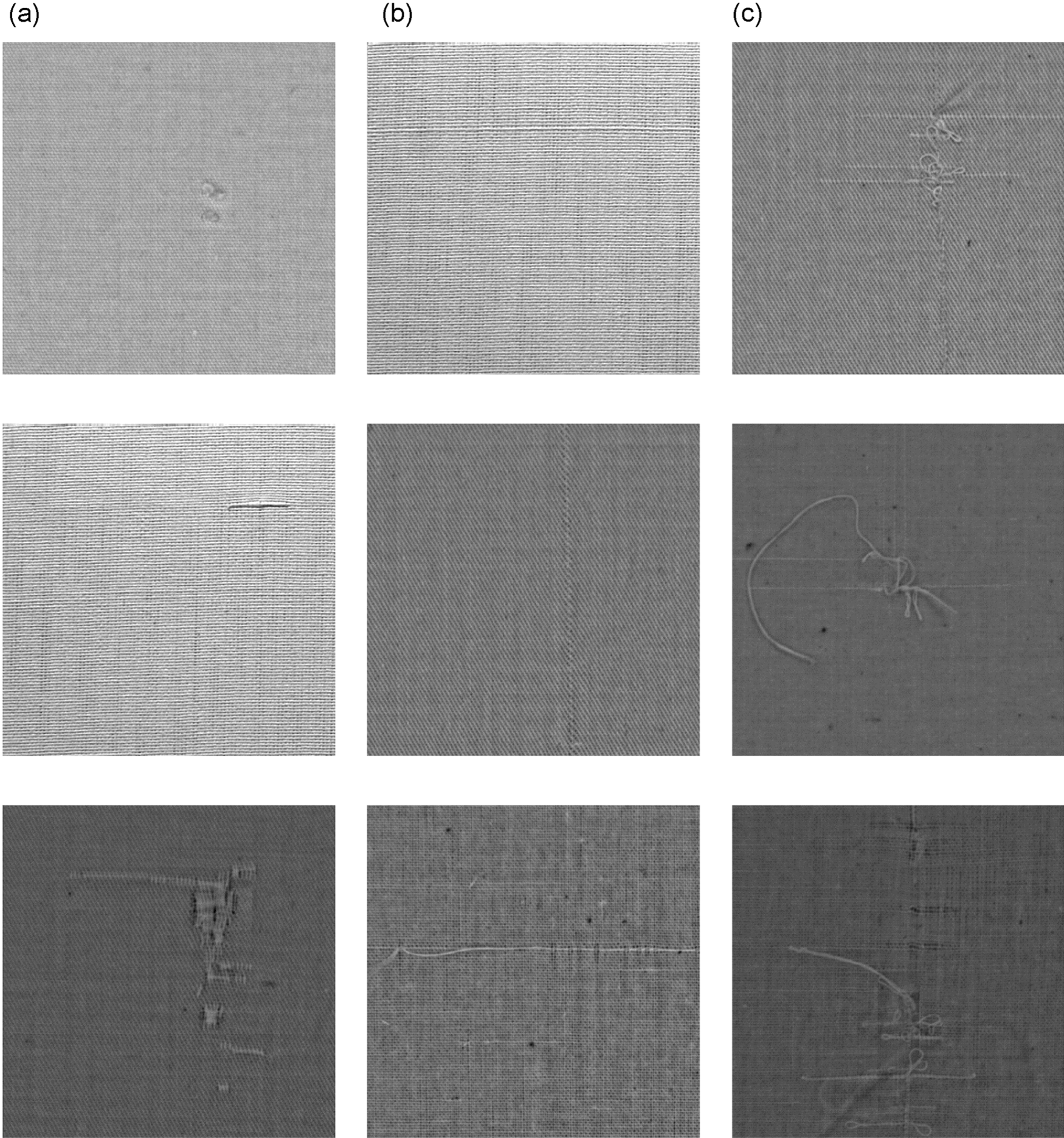

In the experiments, our algorithm performs on each test image and its rotated version separately. The final detection result is the combination of the two detection results from the original image and its rotated version. Note that all detection results of rotated versions are rotated back in order to be consistent with the defects on original images, and 3 × 3 morphological filters are used to remove noise on final binary outputs. The rotation angle is set to 5°, which is found to be adequate to redistribute anomalies, while at the same time suffering very small loss. To select the optimal number of k, we search for the maximum cost function (equation (3)) from 1 to 10 for each analysis, and the upper boundary 10 is sufficient for modeling the textured fabric samples involved in this paper, guaranteeing that optimal k occurs within 10. Considering the effects of noise for calculating μ and σ, we set the constant c = 2.7, making 99.31% of pixels fall into the set interval of equation (4). All experiments were implemented in Matlab (R2009b) on a Linux machine.

Results and discussion

To evaluate the defect detection performance of our algorithm, we examine its adaption on both fabric types and defect types, and a comparison with the algorithm using Fourier reconstruction proposed by Tsai and Hsieh is conducted to confirm the effectiveness of the proposed method,²⁰ where all the parameters used are manually tuned to be optimal. Illustrative detection results for all test samples are presented in Figures 6 to 10, where Figures 6 and 7 concern blocky defects and Figures 8 and 9 correspond to linear defects and mixture of both, respectively. Figure 10 presents detection results for defect-free images. The white regions in Figures 6 to 10 represent the labeled defective regions. Note that each first row of detection results (binary images) in Figures 6 to 10 are obtained by our algorithm and the second are obtained by Fourier reconstruction method.
Figure 6.
Detection results for blocky defects.

Figure 7.
Detection results for blocky defects.

Figure 8.
Detection results for linear defects.

Figure 9.
Detection results for mixture of blocky defects and linear defects.

Figure 10.
Detection results for defect-free images.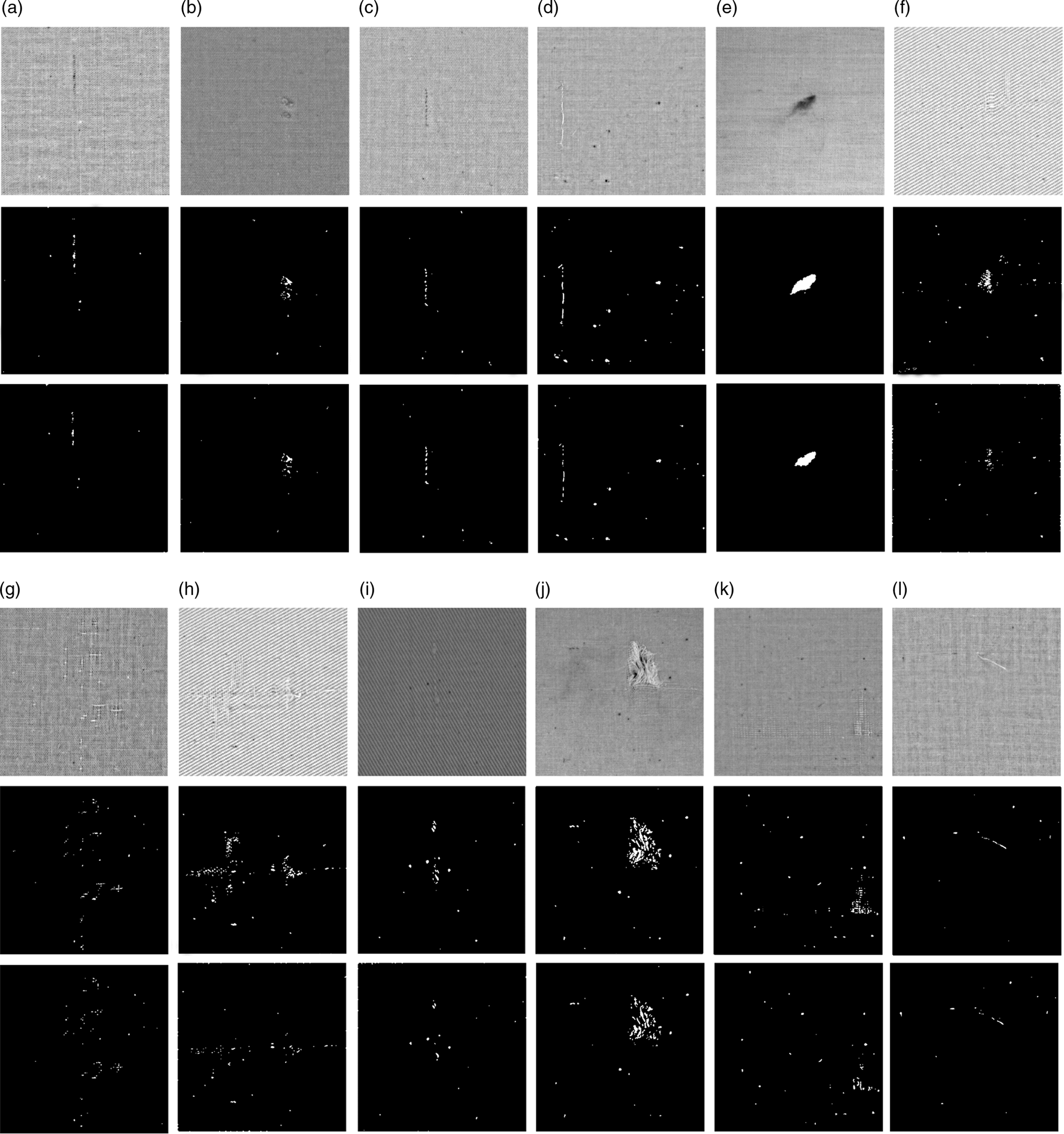

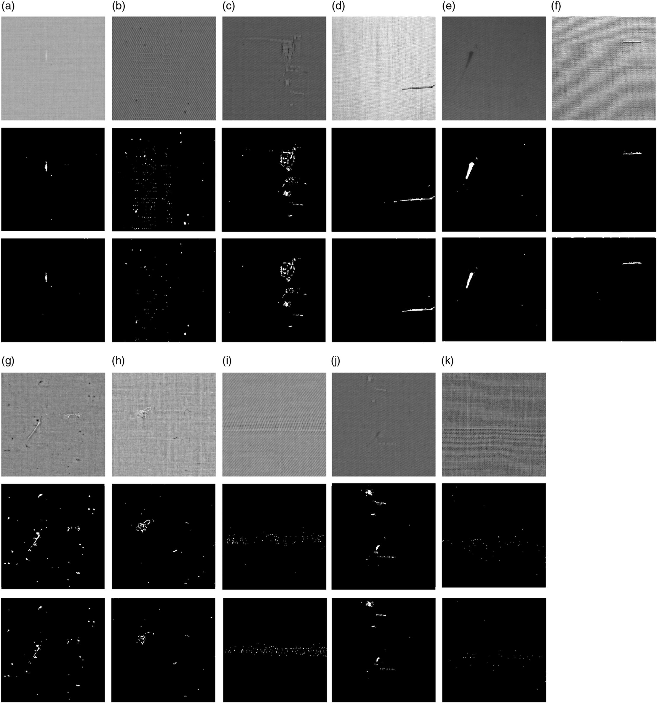
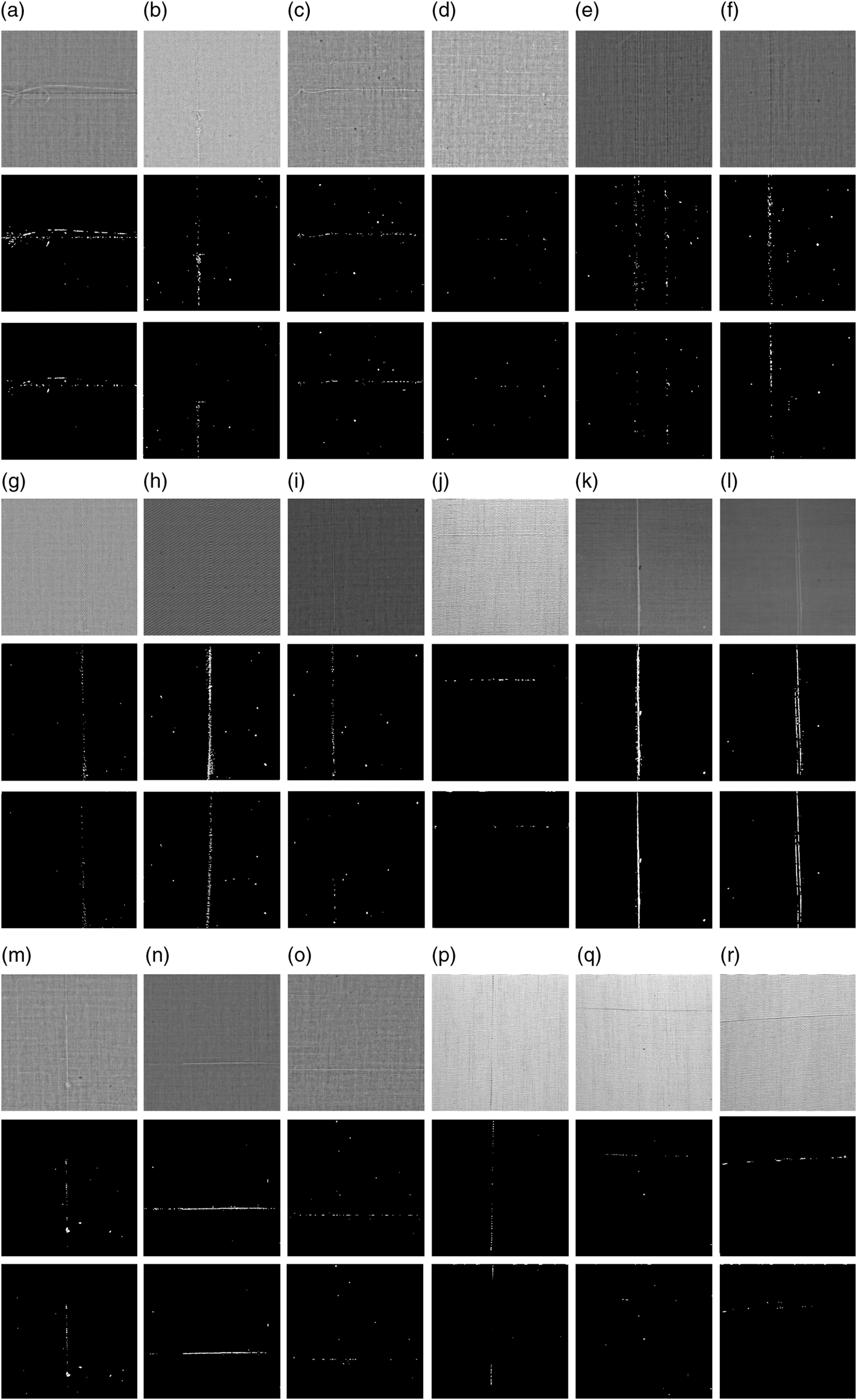
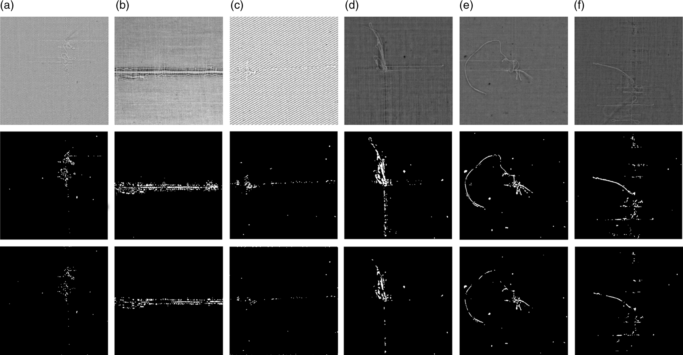
From Figures 6 to 10 it can be seen that our method and the Fourier method achieved quite close detection performance for those defects having great intensity or/and structure change, e.g. Figures 6(d), 6(e), 7(a), 7(d), 7(e), 8(k), and 8(l) for intensity, and for structure, e.g. Figures 6(j), 7(c), 7(f), 7(j), and 9(d). In contrast, for those defects with moderate structure or/and intensity change, our method outperforms the Fourier method, e.g. Figures 6(f), 6(h), 7(h), 8(g), 8(i), and 9(b). The reason for this is that the Fourier method only considers removing the periodic background texture and is not able to enhance defects by increasing their intensity contrast, resulting in poor segmentation as the defective regions in the residual image (background removed) still have low intensity contrast to its background. Another drawback of the Fourier method is that it is sensitive to selected frequency components used to remove background texture. For example, for some plain fabrics, due to the scattering distribution of their Fourier domain, it is quite hard to locate the high-energy frequency components corresponding to its background texture information.

Adaptation to fabric types and defect types

The adaption of fabric types is usually associated with the false alarm rate (FAR). In current context, the false alarm occurs when white pixels appear on the non-defective regions. From Figures 6 to 10, almost all detection results on non-defective areas are accompanied with white pixels which seem to have a high FAR. However, by examining those scattering white pixel regions together with their original images, it can be found that those regions correspond to dark spots on their originals, and those dark spots are caused by shadows of pills on fabric surfaces. Since the dark spots can be avoided by pre-processing, such as washing before inspection or using advanced illumination, when ignoring the effect of the dark spots, both our algorithm and Fourier method can achieve 0% of FAR.

The adaption of defects is of great importance to a defect detection algorithm, which can be understood as the miss detection rate (MDR). In the current context, miss detection occurs when white pixels fail to appear on defective regions.

By examining defects in Figures 6 to 9, it is clear that our algorithm can detect more defect types than the Fourier method, especially for the defects with moderate structure change, showing our algorithm with 12.8% of MDR (fail in Figures 7(b), 7(i), 7(k), 8(d), 8(m), and 8(q)), compared with the Fourier method with 19.1% of MDR (fail in three more samples based on our algorithm: Figured 6(h), 8(e) and 8(i)). By observing the defects in Figures 6(b), (i) and (k), we can see that those defects share large parts of their areas with the defect-free regions, rendering our algorithm ineffective to discriminate those sharing regions, since our algorithm only focuses on identifying the defective regions. One way to eliminate this problem is to perform a further analysis on neighboring information, such as labeling defects based on sub-windows.

By examining undetected regions in Figures 8(d) and (m), it can be found that those regions cause such minor disturbance that they are not accepted as defects. That is to say, our algorithm will be ineffective to detect those defects having inadequate anomalies (i.e. gray-level or structure changes) to be detected, especially for some linear defects. On the other hand, the undetected regions in Figures 8(d) and (m) are also difficult for visual identification, when only taking a look at the columns involving the undetected regions rather than observing them based on the whole image. Furthermore, the reason for the fail of Figure 8(q) and poor segmentation for Figures 8(j), (o) and (r) is mainly due to the tiny size of defects that will be removed like noise (smaller than 3 × 3) by the morphological operation. Hence, in practical applications, we recommend using different filter sizes depending on specific defect size to be detected.

However, since a Fourier transform can be easily done in FFT fashion, the Fourier method is more efficient than our algorithm from a computational complexity point of view, suggesting that our method will be too demanding for a real-time system, especially for the process of selecting dictionary size k. Therefore, some adequate optimizations upon our algorithm are necessary to make it satisfy on-line requirements. For example, in real applications, considering the fabric type could not be changed during an inspection process, one can introduce a training phase to obtain proper parameters before conducting inspection, e.g. using a fixed k or update k during the inspection process to alleviate the computational burden. Of course, using dedicated processors like DSPs or GPUs is another way to speed up processing time.

Conclusion

In this paper, we have presented a new algorithm based on learning adaptive dictionaries to address the fabric defect detection problem. Such a dictionary can efficiently represent columns of normal fabric images using a linear combination of its elements. The proposed method takes advantage of repeated patterns of fabric texture, which can be efficiently modeled by a linear combination of a few elements in terms of image columns. By selecting a proper dictionary size that is able to approximate normal fabric columns well, but poorly for anomalous ones, the defective regions can be easily enhanced in the residual image from which a simple thresholding operation can be used to segment defects straightforwardly. To adapt more defects, we perform our algorithm on a test sample and its rotated version, which has been proven to facilitate identification for linear defects. The primary contribution of the proposed approach is that it does not require any prior information, making our algorithm little sensitive to fabric stretch or illumination change.

Experimental results on 52 real-world fabric images show that our algorithm is more robust in adapting to different defect types, especially for structure change defects, compared to the Fourier reconstruction method. At the same time, the proposed method is quite robust in adapting to different fabric textures and performance mainly depends on defect size and the anomalies against background texture to be present.

Footnotes

Funding

This research was supported by the Fundamental Research Funds for the Central Universities of China.

References

Kumar

. Computer-vision-based fabric defect detection: a survey. IEEE Trans Ind Electron 2008; 55: 348–363.

Mahajan

Kolhe

Patil

. A review of automatic fabric defect detection techniques. Adv Comput Res 2009; 1: 18–29.

Kumar

. Neural network based detection of local textile defects. Pattern Recognit 2003; 36: 1645–1659.

Tolba

. Neighborhood-preserving cross correlation for automated visual inspection of fine-structured textile fabrics. Text Res J 2011; 81: 2033–2042.

Kuo

Lee

. A back-propagation neural network for recognizing fabric defects. Text Res J 2003; 73: 147–151.

Wang

Huang

. Fabric defect detection based on multiple fractal features and support vector data description. Eng Appl Artif Intell 2009; 22: 224–235.

Chan

Pang

GKH

. Fabric defect detection by Fourier analysis. IEEE Trans Ind Appl 2000; 36: 1267–1276.

Tsai

. Automatic inspection of fabric defects using an artificial neural network technique. Text Res J 1996; 66: 474–483.

Yang XZ. Discriminative fabric defect detection and classification using adaptive wavelet. PhD Thesis, University of Hong Kong, China, 2003.

10.

Kim

Kang

. Texture classification and segmentation using wavelet packet frame and Gaussian mixture model. Pattern Recognit 2007; 40: 1207–1221.

11.

Hou Z and Parker JM. Texture defect detection using support vector machines with adaptive Gabor wavelet features. In: Proceedings of the seventh IEEE workshop on applications of computer vision, WACV 2005, art. no. 4129491, pp.275–280.

12.

Huang

Wang

. Detection of fabric defects by auto-regressive spectral analysis and support vector data description. Text Res J 2010; 80: 579–589.

13.

Escofet

Navarro

Millán

. Detection of local defects in textile webs using Gabor filters. Opt Eng 1998; 37: 2297–2307.

14.

Kumar

Pang

GKH

. Defect detection in textured materials using Gabor filters. IEEE Trans Ind Appl 2002; 38: 425–440.

15.

Arivazhagan

Ganesan

Bama

. Fault segmentation in fabric images using gabor wavelet transform. Mach Vision Appl 2006; 16: 356–363.

16.

Bodnarova

Bennamoun

Latham

. Optimal Gabor filters for textile flaw detection. Pattern Recognit 2002; 35: 2973–2991.

17.

Mak

Peng

. An automated inspection system for textile fabrics based on Gabor filters. Robot Comput Integr Manuf 2008; 24: 359–369.

18.

Srikaew

Attakitmongcol

Kumsawat

. Detection of defect in textile fabrics using optimal Gabor wavelet network and two-dimensional PCA. Lect Notes Comput Sci 6939: 436–445.

19.

Bodnarova

Bennamoun

Kubik

. Suitability analysis of techniques for flaw detection in textiles using texture analysis. Pattern Anal Appl 2000; 3: 254–266.

20.

Tsai

Hsieh

. Automated surface inspection for directional textures. Image Vision Comput 1999; 18: 49–62.

21.

Tsai

Huang

. Automated surface inspection for statistical textures. Image Vision Comput 2003; 21: 307–323.

22.

Tsai

Hsiao

. Automatic surface inspection using wavelet reconstruction. Pattern Recognit 2001; 34: 1285–1305.

23.

Sezer

Ercil

Ertuzun

. Automated inspection of textile defects using independent component analysis. Pattern Recognit 2007; 40: 121–133.

24.

Elad

Aharon

. Image denoising via sparse and redundant representations over learned dictionaries. IEEE Trans Image Process 2006; 15: 3736–3745.

25.

Wright

Yang

Ganesh

. Robust face recognition via sparse representation. IEEE Trans Pattern Anal 2009; 31: 210–227.

26.

Cong Y, Yuan J, Liu J. Sparse reconstruction cost for abnormal event detection. In: Proceedings of the IEEE computer society conference on computer vision and pattern recognition, 2011, paper no. 5995434, pp.3449–3456.

27.

Mairal

Bach

Ponce

. et al. Online learning for matrix factorization and sparse coding. J Mach Learn Res 2010; 11: 19–60.