Assessing cotton maturity using distributional parameters of fiber cross-section measurements

Abstract

Many previous studies on cotton maturity used a sole parameter to rank the maturity of a cotton sample containing a large number of fibers. In light of the complexity of maturity distributions, the sole-parameter approach does not appear to be reliable and rational for cotton maturity evaluation. More distributional parameters should be examined and included in the new classification methods. This paper (1) introduces important changes in the image-analysis algorithms for cotton cross-section measurements to enhance the consistency of fiber detections in order to reduce the bias on immature fibers, (2) investigates the characteristics and patterns of cotton maturity distributions, and (3) presents the experimental results on the cross-section images selected from seven cotton varieties that have a wide range of maturities. It is found that the skewness of a maturity distribution is an essential parameter for classifying the distribution pattern and that the dead fiber content and the mature fiber content are the important distributional parameters for assessing cotton maturity.

Keywords

cotton maturity image analysis maturity distribution dead fiber content

There is a relatively long history of efforts to establish a set of standard cottons for calibrating fiber maturity and fineness measurements. In 1956, Lord¹ established 100 cottons to calibrate micronaire. In the 1980s, the International Textile Manufacturers Federation (ITMF), in cooperation with other organizations, developed a set of nine calibration cottons for use in large-scale maturity-round trials.² In 1999, Thibodeaux and Rajasekaran³ used a commercial image-analysis system to measure the cross-sectional images of approximately 50 cotton varieties representing a wide range of genetic finenesses that were grown and hand-harvested in the USA. In the 2000s, Hequet's and Thibodeaux's groups performed a multi-year project to create a larger-scale cotton-maturity reference by analyzing images of the 104 cotton varieties⁴ collected worldwide using a new fiber cross-sectioning protocol⁵ and customized fiber image-analysis software (FIAS).⁶ Now, there is a consensus in the cotton research community that fiber cross-sectional analysis provides fundamental measurements that are directly related to cotton maturity and that this is the most reasonable approach for developing the cotton-reference database. The FIAS helped expedite the analysis on a large quantity of fiber cross-section images and improved the data reliability for calibrating other testing methods.⁴ However, a recent independent study revealed that there is an overestimation of the maturity level of bale cotton by around 9% using the laboratory protocol and the FIAS, because 10–40% of immature fibers could not be detected correctly in the image processing.⁷

Immature fibers, especially dead fibers, have thinner walls, and thus they are more easily scratched or shredded by the cutting blade. They are also likely to be folded up transversely when the lumens collapse, which increases the difficulty of edge detection. Based on the experience of developing and using the FIAS, we know that the FIAS lacks functions that can automatically amend broken edges of cross-sections and that unclosed cross-sections become oblivious in a segmentation routine called “background flooding.” Most of the ignored fibers are immature fibers, which cause a systematic bias in fiber detections, and when a large number of fibers cannot be detected correctly, the cumulative measurements will not realistically reflect maturity distributions of the sample. In addition, the mean value of the cross-section data is often used to indicate the maturity level of a sample.^4,6 In light of the complexity of maturity distributions, the sole-parameter approach does not appear to be reliable and rational for ranking the maturity among different samples.

In this paper, we first present the modified algorithms made in the current version of FIAS to improve its robustness and accuracy of detecting fiber cross-sections, including those with obscure and incomplete boundaries, in order to increase the total number of valid measurements and reduce the bias on immature fibers. We then examine the basic patterns of maturity distributions based on the skewness of the distribution and propose a way to calculate various fiber contents (such as dead fiber and mature fiber contents (MFCs)) in the distribution. The paper also presents comparisons between the previous version and the current version of FIAS in fiber detections and in maturity statistics.

Method

In the cross-sectional analysis, the maturity of individual fibers is often measured by a shape factor called circularity or the theta (θ) value.^3,4,6,8 The θ is determined by the perimeter (P) and the net area (A) of a fiber cross-section (θ = 4πA/P²),⁹ which indicates the degree of wall thickening. Thus, in this paper θ is referred to as cotton maturity. Increasing the accuracy of locating fiber boundaries and lumens is paramount for obtaining reliable maturity measurements.

The images of fiber cross-sections used in this study were provided by the Fiber and Biopolymer Research Institute (FBRI) of Texas Tech University. A total of 15,473 images from the seven cotton varieties were tested with the previous and current FIAS software to examine the differences in the number of detected fibers, the maturity correlation with the data obtained from the Advanced Fiber Information System (AFIS), and the High Volume Instrument (HVI), as well as the distributional parameters. Each of the seven varieties was assigned a unique four-digit symbol (e.g., 2996, 2999…).

Modification of fiber-detection algorithms

To segment individual fiber cross-sections in the image, the FIAS has four major image-processing routines: (1) dynamic thresholding; (2) background flooding; (3) skeletonizing fibers; and (4) identifying lumens.⁷ These routines appear to be effective when image illumination is uniform and image contrast is sufficient, but they are not robust enough for fibers that have low contrast, broken edges, or distorted cross-sections due to self-folding/wrapping of fiber ribbons. Routines (2) and (3) are more standardized procedures with fewer adjustable parameters, and therefore we focused on improving routines (1) and (4), which are responsible for locating accurate fiber boundaries and lumens. An edge-amending routine was also added to connect narrowly broken boundaries to prevent them from disappearing in the background flooding.

Adaptive thresholding

Illumination intensity in a captured eight-bit gray-scale image can vary drastically. There is no universal threshold that can generate consistent results across the entire image. The dynamic threshold method with adaptive parameters is a reasonable way to convert an eight-bit gray-scaled image into a binary one. In the previous FIAS,⁶ a sub-window of a given size was used to calculate the threshold (T_i) to separate object pixels in the window from the background. T_i was determined by both the mean M_i and the standard deviation SD_i of pixel intensities in the window, as follows:

T_{i} = M_{i} - c \times {SD}_{i},

(1)

where c was a coefficient that was set as 0.2 in the program.⁶ The window size was also fixed at 7 × 7 pixels. Since both c and the window size were not changeable despite differences in intensity variability, T_i calculated using Equation (1) might not always be optimal for generating binary images. Figure 1(a) displays an image with non-uniform illumination, and Figure 1(b) is the resultant image with this threshold method. The high level of noise in Figure 1(b) makes the tracing of fiber boundaries extremely difficult. It seems that in Figure 1(a) darker regions are more sensitive to background noise than brighter regions. The coefficient c should be adaptive to the mean intensity (M_i) of the window around the active pixel to adjust the sensitivity of thresholding. Based on the observations of many images, it was found that a brighter region normally has a lower noise level than a darker region, and thus c for a brighter window should be increased to lower T_i. The location-dependent c is denoted as c_i. By trial and error with a wide range of images, we established the following empirical equation for the calculating c_i based on M_i:

c_{i} = 0.014 M_{i} - 2.694 (R^{2} = 0.9857) .

(2)

Figure 1.

Adaptive thresholding: original image (a); previous binary image (b); and improved binary image (c).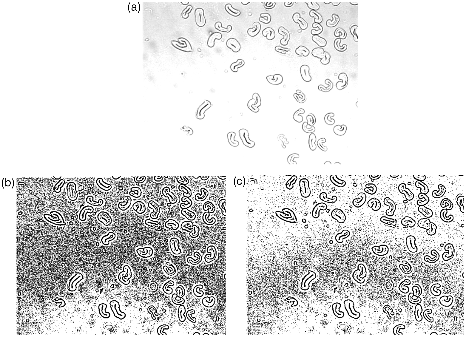

The binary image of Figure 1(a), with the aid of dynamic coefficient c_i, is displayed in Figure 1(c), in which the large proportion of the noisy image (Figure 1(b)) was reduced. Fiber boundaries in this image are also more complete than those in Figure 1(b).

Amending broken edges

As seen in Figure 1(c), the binary image still contains much background noise and small objects such as broken edges of fibers, which need to be removed so that only enclosed fiber boundaries are present. This can be done efficiently with a procedure called “background flooding,” which fills the white background with black pixels. Broken fibers are also absorbed by the “flooding” when their inner white regions (fiber walls) are occupied by black pixels. In order to keep those narrowly broken fibers from being eliminated, a step to amend almost-connected edges needs to be added.

There is no generic algorithm for detecting the ends of broken boundaries. The edge-amending routine had to be developed on a case-by-case basis after fiber outer boundaries were traced, and it mainly involved three steps, as follows. Step 1 is to check whether a fiber boundary has a “dead-end” pixel by counting the number of its neighboring pixels. A dead-end pixel is the one that has one neighbor in the boundary chain. Step 2 involves searching for another “dead end” in the same chain. Finally, step 3 consists of checking that the open distance between the two is within an allowable limit and that the boundary length between the two exceeded the threshold on the fiber perimeter. The last step is meant to prevent a connection between two dead ends that are not on the same boundary or are too far apart. The connection distance was limited to five pixels in the new program, and it was simply made with a straight line drawn automatically to join the two identified dead ends.

Figure 2(a) shows a few examples of typical broken boundaries, and Figure 2(b) shows the connections made. The connection lines do not alter the fibers' original shapes but prevent them from being immersed with the background flooding.

Figure 2.

Broken boundaries (a) and amended connections (b).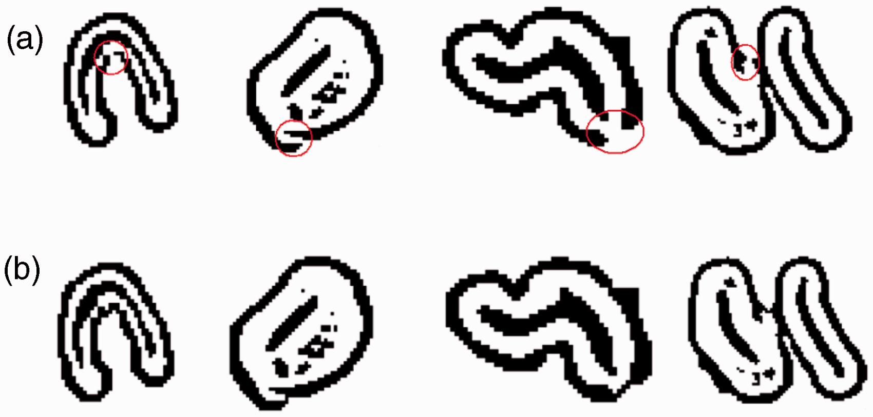

Identifying lumens

In a cross-section image, often some fibers do not possess visible lumens. As seen in Figure 3(a), fibers 1, 2, and 3 are immature fibers with lumens that are totally collapsed; fibers 4, 5, and 6 do not exhibit clear lumens because of low contrasts; and fibers 7, 8, and 9 show partial lumens. Lumen areas in these fibers can be readily overestimated or underestimated.

Figure 3.

Original image (a) and detected cross-sections (b).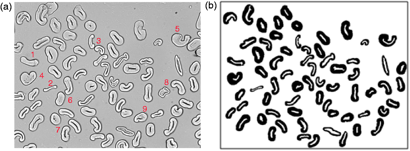

Once a fiber boundary is located, another threshold is calculated by using only the pixels within the boundary so that the lumen can be more precisely segmented with localized parameters (the mean and standard deviation of the pixel intensities). Since a lumen should be situated in the fiber center, the skeleton of the fiber—that is, the middle axis of the fiber—can be used to locate the lumen if multiple black areas are present inside the boundary. The skeletons of fibers with lumens that are not detected after the thresholding (one-pixel-thick line segments) are placed as lumens. This localized thresholding and skeletonizing enhances the accuracy of lumen size and location (Figure 3(b)).

Table 1 lists a few examples of fiber detection results obtained from the previous and current versions of FIAS. The fibers in the “Original” culumn were cropped out of the selected images prior to any processing, and the fibers in the “Previous” and “Current” were the corresponding regions cropped from the images processed by the previous and current FIAS, respectively. It is evident that the previous FIAS is likely to miss adherent fibers, and often under- or over-estimates lumens. With the improved algorithms, the current FIAS is more robust in separating adherent fibers, and more accurate in locating lumens.

Table 1.

Comparison of fiber detection results of two versions of fiber image-analysis software

Characteristics of maturity distributions

A regular image of 640 × 480 pixels normally contains a number of fiber cross-sections that varies between 10 and 100. The θ values of cross-sections in multiple images are measured individually, and the frequencies are counted on a scale of [0, 1]. After a sufficient number of fiber cross-sections are measured from multiple images, the descriptive statistics of fiber maturity data (θ), including the mean M_θ, the standard deviation (SD_θ), the skewness (S_θ), and the kurtosis (K_θ), can be used to examine the features of maturity distribution. For a unimodal distribution, the mean and standard deviation describe the central tendency and the variability of the distribution, while skewness and kurtosis indicate the symmetry and the “peakedness” of the distribution. According to the imbalance situation in a frequency distribution, skewness can be negative, positive, or zero. A negative skew indicates that the distribution is left skewed (i.e., the data concentrate more on the right-hand side of the mean), a positive skew corresponds to the opposite case, and a zero skew indicates that the tails on both sides of the mean balance out, which is due to the symmetry or the even-out asymmetries. A high kurtosis corresponds to a distribution with a sharp peak and long tails, while a low kurtosis indicates a distribution with a round peak and short, thinner tails. When either skewness or kurtosis significantly deviates from the value corresponding to the normal distribution, the normality of the distribution diminishes. For a non-normal distribution, many classical statistical tests, such as t-tests, F-tests, and chi-squared, tests may not be applicable.

Figure 4 displays the maturity (θ) distributions of two cotton samples (the sample codes are 3044 and 3055), in which the x-axis represents the fiber maturity and the y-axis represents the percentage of totally detected fibers. The θs of cotton 3044 and cotton 3055 have almost the same mean (M_θ = 0.475 and 0.479), standard deviation (SD_θ = 0.180 and 0.172), and kurtosis (K_θ = −0.535 and −0.532), but different skewness values (S_θ = 0.367 and 0.232). Obviously, these two cottons have very distinctive θ distributions, as shown in Figure 4, and their maturity levels should not be rated only by the mean θ values. Cotton 3044 contains more immature fibers than cotton 3055, although they have the same M_θ. Thus, distributional information must be taken into account when comparing or ranking maturities of different cottons.

Figure 4.

θ distributions of cottons with the same M_θ, SD_θ, and K_θ, but different S_θ.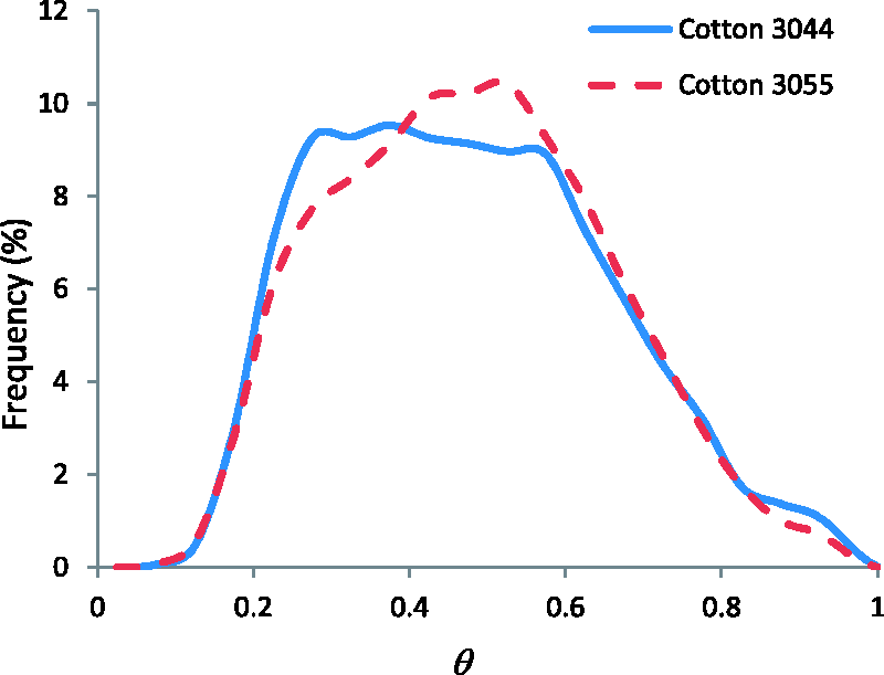

Patterns of maturity distributions

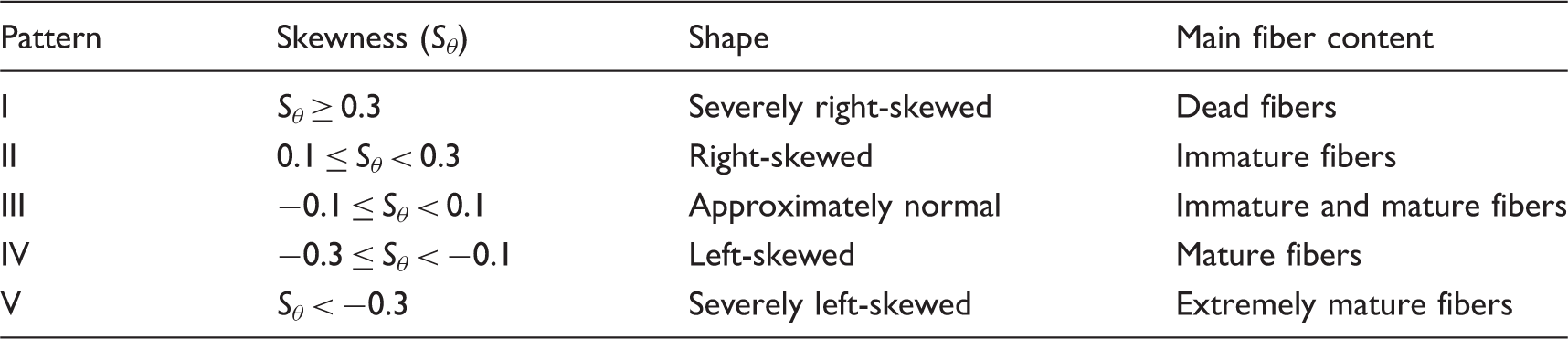
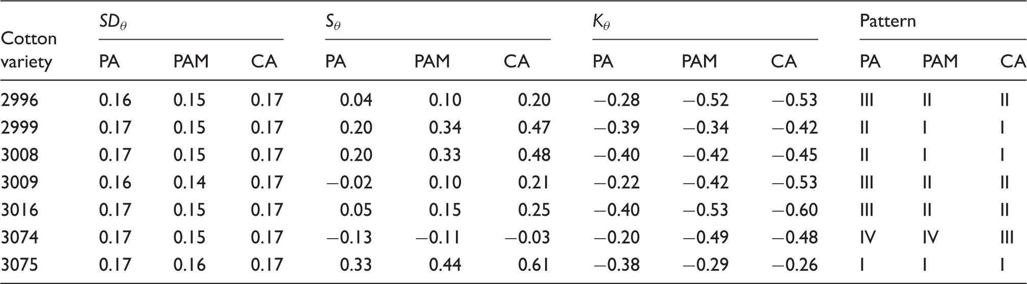
As indicated in Figure 4, the maturity distributions of different cotton samples can have substantially different shapes. Among the parameters describing the shape of a distribution, skewness is the first principal component that distinguishes distribution patterns notably. Five patterns can be defined to categorize maturity distributions based on skewness values (S_θ), as listed in Table 2. From the data of the available samples, it can be observed that when S_θ is in the range of (−0.1 to 0.1), the distribution takes a shape approximate to the normal distribution (pattern III). When S_θ < −0.3 or S_θ > 0.3, the distribution is severely either right-skewed (pattern I) or left-skewed (pattern V). There is one intermediate pattern between patterns I and III, and one between patterns III and V, and each pattern indicates concentrated fiber contents in the distribution. For example, pattern I reveals that the main fiber content is “dead fiber” (extremely immature), while pattern V reflects a large number of extremely mature fibers. Figure 5 displays five maturity distributions to give one sample for each of these patterns. Only the distribution in pattern III is deemed to be approximately normal. These five patterns represent five classes of cotton maturity, which are differentiated by not only the mean values but also the other distribution parameters.

Figure 5.

Patterns of maturity distributions.

Table 2.

Maturity distribution patterns

Pattern	Skewness (S_θ)	Shape	Main fiber content
I	S_θ ≥ 0.3	Severely right-skewed	Dead fibers
II	0.1 ≤ S_θ < 0.3	Right-skewed	Immature fibers
III	−0.1 ≤ S_θ < 0.1	Approximately normal	Immature and mature fibers
IV	−0.3 ≤ S_θ < −0.1	Left-skewed	Mature fibers
V	S_θ < −0.3	Severely left-skewed	Extremely mature fibers

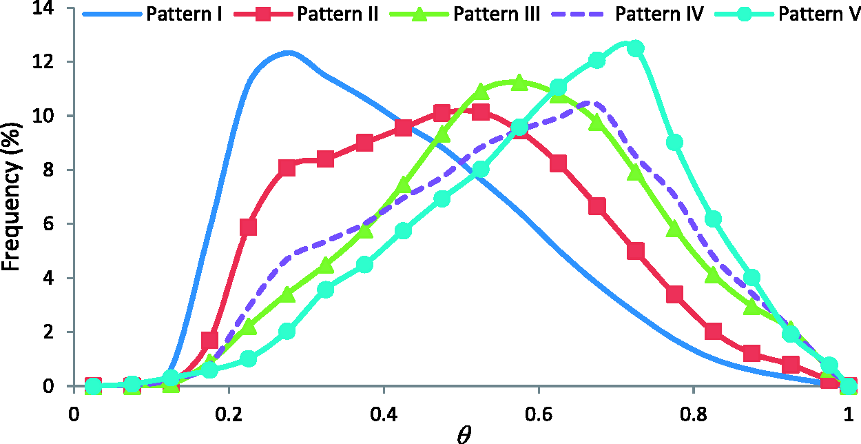
Fiber types and contents

Based on visual characteristics of cotton cross-sections, we may categorize fibers into three general types: dead, immature, and mature. Table 3 lists four examples and the corresponding range of their θ values for each fiber type. Dead fibers refer to extremely immature cotton fibers, the development of which is terminated at an early stage of their life. Dead fibers have thin secondary walls and look like flat ribbons when collapsed, and their θ values are normally under 0.3 (the top row in the table). Immature fibers are those growing to a certain degree and having apparent fiber walls and lumens (the middle row). The typical θ values of immature fibers range from 0.3 to 0.6. Mature fibers refer to those fully grown fibers with round or oval shapes and small lumens (the bottom row in the table). Normally, the θ value of a mature fiber should exceed 0.6. Therefore, dead, immature, and mature cottons can be simply classified according to their θ values.

Table 3.

Fiber types based on θ values

Compared with mature fibers, dead fibers are more easily entangled to form neps,¹⁰ which decrease the efficiency of yarn spinning and the uniformity of yarn structure. Neps also have an accelerated rate of desorption due to a lack of cellulosic content, and thus they are unable to retain colorants after dyeing.¹¹ Dead fiber is the main cause of white speck problems in a dyed fabric.^12,13 White specks usually result in a major discount in price for the manufacturer. On the other hand, mature fibers offer better strength and dyeability, and should be at a premium in terms of the ultimate assessment of cotton maturity. Therefore, the dead fiber content (DFC), immature fiber content (IFC), and MFC in cotton are the important indicators of fiber quality. The three fiber contents can be obtained by adding the relative probabilities within the three separate θ ranges, as illustrated in Figure 6.

Figure 6.

Contents of dead, immature, and mature fibers in a maturity distribution.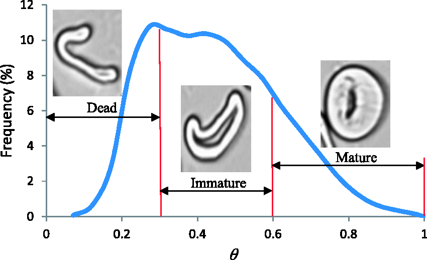

Results and discussion

In this paper, the tests performed with the previous and current FIAS analyses were denoted as PA and CA, respectively. Because the previous FIAS was not able to identify correctly many of the fiber cross-sections that had unclear or incomplete boundaries, a manual editing function was added to allow the user to remove mistaken cross-sections from the processed image on the screen. When the mouse was double-clicked on a fiber, the cross-section could be marked, and the corresponding data were deleted from the output. The PA test after the manual removal was symbolized as PAM data, which were provided by FBRI. The current FIAS improves the fiber-detection functions and can automatically delete wrong cross-sections even if they are initially detected. It also has a set of manual editing tools to assist the user in amending unclear boundaries, detaching connected fibers, and deleting anomalous objects using a mouse or a tablet pen. The manual editing can be repeated until the visual examination on all the fibers is satisfied, and the manual editing process after the CA test is called CAM, the results of which can be regarded as the most trustful data for assessing the accuracy of the CA data.

The 2201 images of cotton variety 2996 were selected to perform the CA and CAM tests, and these images were first batch-processed by the current FIAS and then manually edited image by image. Figure 7 displays the θ histograms of the CA and CAM tests and the descriptive statistics (M_θ,, SD_θ, S_θ, and K_θ). Although slight discrepancies in fiber frequency can be observed near θ = 0.3, the agreement of the two histograms is extremely high (R² = 0.999), and the two sets of the descriptive statistics are approximately identical. This proves that the CA test is able to produce reliable fiber detections, except for irreparable immature cross-sections. Because of the high agreement between the CA and CAM data, there is no need to perform manual editing after the CA test.

Figure 7.

θ histograms and the descriptive statistics of cotton 2996 in the CA and CAM tests.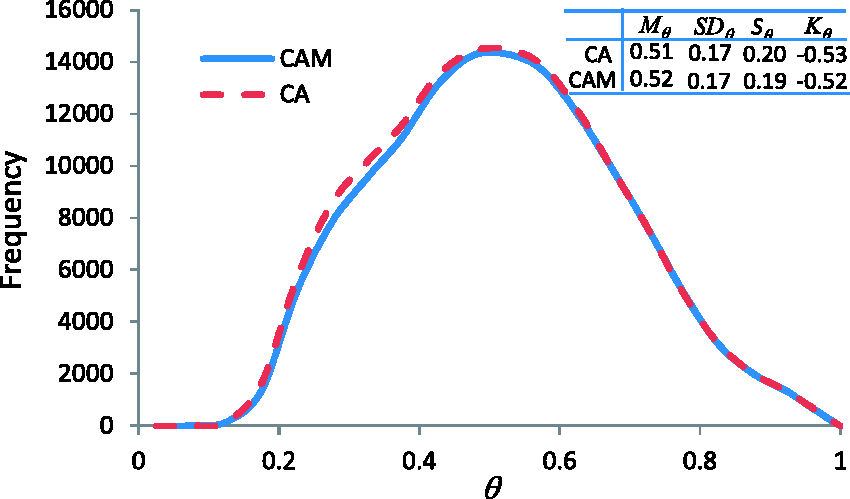

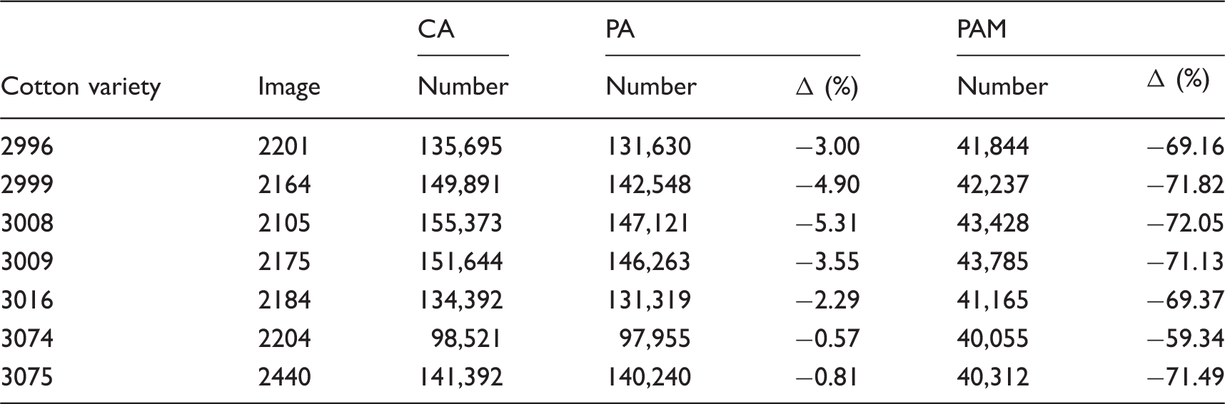
Table 4 displays the numbers of fibers identified in the CA, PA, and PAM tests, respectively, from the same set of images of the seven cotton varieties. In the table, Δ is the difference in the fiber numbers between the PA (or PAM) test and the CA test divided by the fiber number of the CA test. Compared with the CA numbers of detected fibers in the seven varieties, the PA numbers have reductions varying from 0.57% to 5.31%. After the manual deletion of wrong cross-sections, the numbers in the PAM dramatically decrease by more than 59%. This means that the improved FIAS can salvage many more fibers, most of which are immature fibers, and alleviate the previous bias on immature fibers in the maturity distribution.

Table 4.

Comparisons in number of the identified fibers

Cotton variety	Image	CA	PA		PAM
Cotton variety	Image	Number	Number	Δ (%)	Number	Δ (%)
2996	2201	135,695	131,630	−3.00	41,844	−69.16
2999	2164	149,891	142,548	−4.90	42,237	−71.82
3008	2105	155,373	147,121	−5.31	43,428	−72.05
3009	2175	151,644	146,263	−3.55	43,785	−71.13
3016	2184	134,392	131,319	−2.29	41,165	−69.37
3074	2204	98,521	97,955	−0.57	40,055	−59.34
3075	2440	141,392	140,240	−0.81	40,312	−71.49

Table 5 presents the mean θ values (M_θ) of the seven cottons in the three tests together with the AFIS maturity ratios (M_r) and the HVI micronaire. The M_θ values of the PA test are all higher than those in the PAM or CA test. This is because in the PA test more immature fibers were wrongly detected as mature fibers. By removing those incorrect fibers manually, the PAM lowered the M_θ values, which are still slightly higher than those in the CA. However, the M_θ values of all three tests are highly correlated with each other and have almost the same linear R² as the AFIS maturity ratios. The CA and PAM tests noticeably improved the R² (quadratic) between the M_θ and the micronaire. Table 5 also provides the maturity ratios calculated from the M_θ values (M_r = M_θ/0.577)⁴ for direct comparisons with the M_r values of AFIS. It appears that the M_r values from the PA test are higher than those of AFIS, except for cotton 3075, while the M_r values from the CA test are lower than those of AFIS, except for cotton 3074.

Table 5.

Comparisons in mean maturity (M_θ)

Cotton variety	M_θ			M_r				High Volume Instrument Micronaire
Cotton variety	PA	PAM	CA	PA	PAM	CA	AFIS	High Volume Instrument Micronaire
2996	0.54	0.52	0.51	0.94	0.90	0.88	0.90	4.60
2999	0.48	0.45	0.45	0.83	0.78	0.78	0.80	3.30
3008	0.50	0.47	0.46	0.87	0.81	0.80	0.84	3.20
3009	0.55	0.52	0.51	0.95	0.90	0.88	0.91	3.90
3016	0.52	0.5	0.49	0.90	0.87	0.85	0.86	4.38
3074	0.58	0.57	0.57	1.01	0.99	0.99	0.95	5.65
3075	0.44	0.42	0.42	0.76	0.73	0.73	0.80	3.09
R² with AFIS M_r ^a	0.93	0.95	0.94
R² with micronaire^b	0.82	0.90	0.90

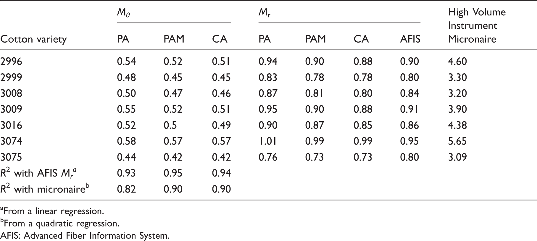
From a linear regression.

From a quadratic regression.

AFIS: Advanced Fiber Information System.

Table 6 presents the other three descriptive parameters of the θ distribution—stand deviation (SD_θ), skewness (S_θ), and kurtosis (K_θ)—which are measured in the PA, PAM, and CA tests, respectively. The PA and CA had almost equivalent SD_θ, values, but both were higher than those in the PAM because anomalous objects were deleted in the PAM, thus causing the θ variations to be reduced. It is interesting to know that the SD_θ values of the seven cottons in the CA are identical. The CA exhibited higher S_θ values than the PA and PAM. Except for cotton 3074, the S_θ values of the remaining six cotton varieties in the CA test are all positive (right-skewed) and are normally twice those in the PA test, causing most of the θ distribution patterns to be shifted by one level. The K_θ values were calculated using the definition of “excess kurtosis,” which is an adjusted version of the kurtosis (minus 3) to make the kurtosis of the normal distribution equal to zero. When the K_θ in a distribution is negative, the distribution has a platykurtic shape—that is, a flatter peak around its mean. According to the K_θ values in the table, the θ distributions of the seven cottons in the three tests are all platykurtic.

Table 6.

Distribution parameters of maturity

Cotton variety	SD_θ			S_θ			K_θ			Pattern
Cotton variety	PA	PAM	CA	PA	PAM	CA	PA	PAM	CA	PA	PAM	CA
2996	0.16	0.15	0.17	0.04	0.10	0.20	−0.28	−0.52	−0.53	III	II	II
2999	0.17	0.15	0.17	0.20	0.34	0.47	−0.39	−0.34	−0.42	II	I	I
3008	0.17	0.15	0.17	0.20	0.33	0.48	−0.40	−0.42	−0.45	II	I	I
3009	0.16	0.14	0.17	−0.02	0.10	0.21	−0.22	−0.42	−0.53	III	II	II
3016	0.17	0.15	0.17	0.05	0.15	0.25	−0.40	−0.53	−0.60	III	II	II
3074	0.17	0.15	0.17	−0.13	−0.11	−0.03	−0.20	−0.49	−0.48	IV	IV	III
3075	0.17	0.16	0.17	0.33	0.44	0.61	−0.38	−0.29	−0.26	I	I	I

Let us take the θ histograms of cotton 2999 in the PA, PAM, and CA tests as an example (see Figure 8). Although the M_θ values in these tests are similar (0.48, 0.45, and 0.45, respectively), their histograms are distinctively different. The CA histogram is severely right-skewed with a sharp peak in the dead fiber range (θ < 0.3), while both the PA and PAM histograms are only slightly right-skewed. Compared with the other two histograms, the PAM histogram has much lower fiber counts because of the removal of wrongly detected fibers.

Figure 8.

θ histograms of cotton 2999 in the PA, PAM, and CA tests.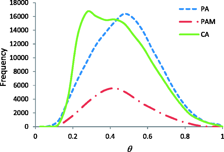

The maturity distributions of the seven cottons in the CA test are displayed in Figure 9, showing diversified distributions from an approximately normal curve (cotton 3074) to a heavily right-skewed curve (cotton 3075). The shape difference of these two cottons are reflected by their S_θ values, which are −0.03 for cotton 3074 and 0.61 for cotton 3075. Of the seven cotton samples, there are two pairs that have similar distributions: cotton 2996/cotton 3009 and cotton 2999/cotton 3008. In each pair, the distribution descriptors M_θ, SD_θ, S_θ, and K_θ of the two samples are greatly comparable. The distribution of cotton 3016 has the flattest top among this group, corresponding to its large negative K_θ (−0.60). When assessing the maturity levels of different samples, one must include all of the four descriptors.

Figure 9.

θ distributions of the seven cottons in the CA test.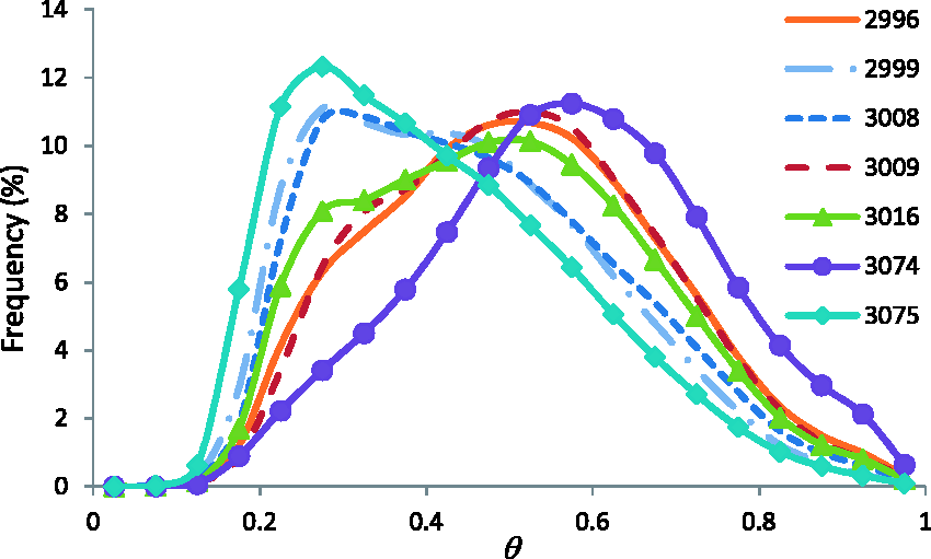

Fibers can be classified by θ values into three simple types (dead, immature, and mature), and the content (proportion) of each type in a sample can be calculated from its θ distribution. Table 7 presents the fiber contents of the seven cotton varieties in the PA, PAM, and CA tests. Immature fibers are the major bodies in the three distributions across the seven cottons, taking more than 50% of the total identified fibers, except in cotton 3074. However, the IFC does not correlate well with the M_θ in the three tests. On the other hand, the DFC and the MFC highly correlate with the M_θ, indicating that these two parameters are more consistent with the overall maturity level. Note that all of the DFC's R values are negative, while the MFC's values are positive. From the PA and CA tests, the DFC increased by a percentage, varying between 0.87% for cotton 3074 and 6.96% for cotton 3008, and the MFC decreased by a percentage, varying between −2.14% for cotton 3074 and −6.78% for cotton 3009. These changes indicate that the current FIAS is able to detect more dead fibers and to avoid detecting wrong objects as mature fibers. A frequently encountered error in the PA test is that the outer boundaries of folded dead fibers (narrow stripes) are likely to be traced and falsely counted as mature fibered (see the example in the bottom row of Table 1), distorting both the DFC and the MFC in the distribution.

Table 7.

Contents of dead, immature, and mature fibers

Cotton Variety	PA (%)			PAM (%)			CA (%)
Cotton Variety	Dead	Immature	Mature	Dead	Immature	Mature	Dead	Immature	Mature
2996	7.98	56.90	35.12	6.94	62.80	30.26	11.76	57.41	30.83
2999	15.45	60.92	23.63	16.38	66.44	17.18	23.06	57.92	19.02
3008	13.11	59.63	27.26	13.97	65.83	20.20	20.07	57.69	22.24
3009	6.71	56.14	37.15	5.84	65.15	29.01	10.87	58.76	30.37
3016	10.50	57.02	32.48	10.65	63.48	25.87	15.80	56.64	27.56
3074	5.72	47.97	46.31	3.54	52.42	44.04	6.59	49.23	44.17
3075	23.02	58.21	18.77	23.28	62.25	14.47	29.91	54.78	15.31
R ^a	−0.91	−0.86	1.00	−0.95	−0.70	0.99	−0.97	−0.52	1.00

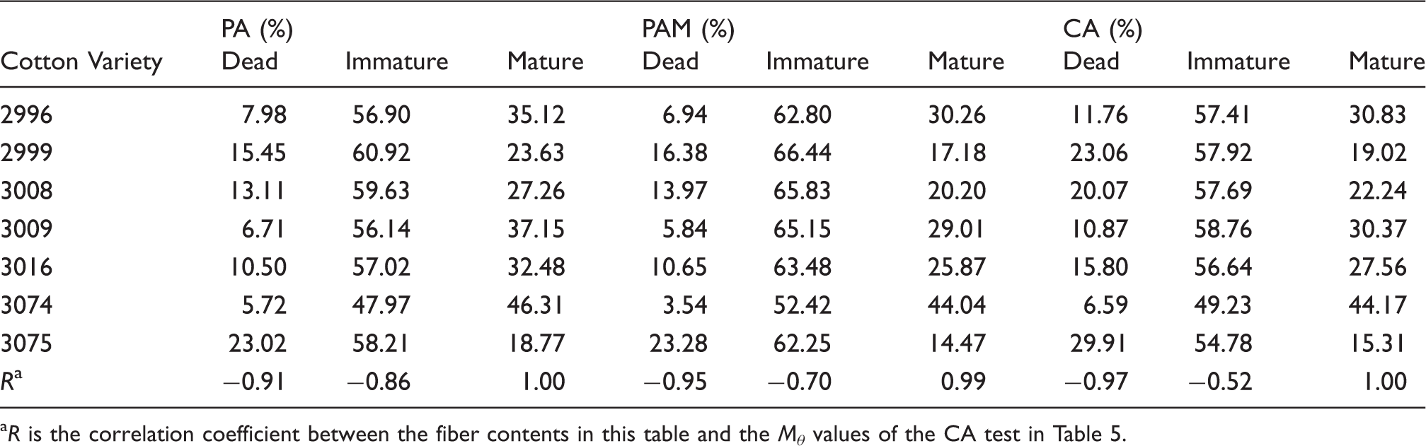
R is the correlation coefficient between the fiber contents in this table and the M_θ values of the CA test in Table 5.

Conclusions

The algorithm changes made in the current FIAS improved the consistency in detecting fibers of various maturities and effectively reduced the bias on immature fibers in previous maturity distributions. The maturity distribution generated in the CA test was correlated highly with that of the manually traced fibers (R² = 0.999). The dramatic reduction in the number of wrong fiber detections eliminates the need for manual editing in a routine test.

The maturity level of a large quantity of cotton fibers should be evaluated with multiple distributional parameters, because any single parameter is insufficient in characterizing the maturity and is often invalid when the distribution is not normal. The basic shapes of cotton maturity distributions can be categorized into five patterns, each representing a major class of cotton maturity. In the same class, the maturities of different samples can be ranked. The skewness of a maturity distribution is an essential parameter to classify the distribution pattern. Most cotton varieties exhibit positively skewed distributions, indicating more IFCs than mature ones.

From a maturity distribution, the contents of dead (DFC), immature (IFC), and mature (MFC) fibers can be calculated by adding the relative probabilities in the specific θ ranges. It seems that IFC is the major body of the maturity distributions for most cotton samples, but only the DFC and the MFC highly correlate with the M_θ—the overall maturity level. Since dead fibers lack strength and dyeability, the DFC should be a discount factor in maturity evaluation. On the other hand, the MFC should be used as a premium in the ultimate rating of fiber quality.

Footnotes

Funding

This work was supported by Cotton Inc. (grant number 13-585).

Acknowledgment

The authors would like to thank Dr Eric Hequet at the FBRI of Texas Tech University for the images and the tested data of the seven cotton samples used in this research.

References

Lord

. Airflow through plugs of textile fibers. Part II. The micronaire test of cotton. J Textil Inst 1956; 47: T16–T47.

Boylston

Thibodeaux

Evans

. Applying microscopy to the development of a reference method for cotton fiber maturity. Textil Res J 1993; 63: 80–87.

Thibodeaux

Rajasekaran

. Development of new reference standards for cotton fiber maturity. J Cotton Sci 1999; 3: 188–193.

Hequet

Wyatt

Abidi

. Creation of a set of reference material for cotton fiber maturity measurements. Textil Res J 2006; 76: 576–586.

Boylston

Evans

Thibodeaux

. A quick embedding method for light microscopy and image analysis of cotton fibers. J Biotechnic Histochem 1995; 70: 24–27.

Huang

. Image analysis for cotton fibers Part II: cross-sectional measurements. Textil Res J 2004; 74: 409–416.

Padmaraj

Krifa

. Evaluating immature fiber bias in fiber cross-section analysis. In: proceedings of the beltwide cotton conferences 2011, pp. 1476–1476.

Matic-Leigh

Cauthen

. Determining cotton fiber maturity by image analysis, Part I: Direct measurement of cotton fiber characteristics. Textil Res J 1994; 64: 534–544.

Pierce

Lord

. The fineness and maturity of cotton. J Textil Inst 1939; 30: 173–210.

10.

Frydrych M Matusiak and Świech T. Cotton Maturity and Its Influence on Nep Formation. Textil Res J 2001; 71: 595–604.

11.

Cheek

Wilcock

. Relationship between direct dye characteristics and coverage of immature fiber neps in dyed cotton fabric. J Soc Dyers Colorists 1988; 104: 477–477.

12.

Peter

Bowes

. Quality variations in cotton and their effects on bleaching, dyeing and finishing. Melliand Textilberichte 1989; 70: 135–137.

13.

Bel

Yao

. White speck potential for mechanically harvested cottons. AATCC Rev 2011; 11: 59–65.