Formulas to determine fabric bending rigidity from simple tests

Abstract

Formulas are derived for effective bending rigidity and bending length, based on the deformation of fabric strips in simple tests. The nine types of tests (including some new ones) involve a cantilever, heart loop, hanging pear loop, hanging ring, free fold, clamped fold, standing wrinkle (buckle), hanging wrinkle, and standing ring. No loads are applied and no special equipment is needed. Only the height of the deformed strip needs to be measured, along with the strip’s length, width, and weight. The results can be applied with different lengths of strips and different orientations (e.g., weft, warp, and bias directions). In the analysis, the fabric strip is modeled as an inextensible elastica. Polynomial approximations are developed that give the value of a nondimensional weight parameter (involving the weight, length, width, and bending rigidity) as a function of the height-to-length ratio. The bending rigidity and bending length can then be directly computed.

Keywords

fabric tests bending rigidity bending length numerical analysis elastica

The classic paper by Peirce¹ proposed various tests to determine the bending rigidity and bending length of fabrics. These include cantilever tests, a heart loop test, a hanging pear loop test, and a hanging ring test. According to Lammens et al.,² Peirce’s formula for the basic cantilever test is not very accurate unless the specific weight of the fabric is small. The same is true for the heart loop test, hanging ring test, and especially for the hanging pear loop test, as was shown by Takatera and Shinohara³ and will be confirmed here. The present paper develops formulas for these and other tests (including some new tests), simply involving measurement of the height (vertical deflection) of the deformed fabric strip in various configurations (along with measurement of the length, width, and weight of the strip).

Assume that the strip is thin and uniform with length L, constant weight w per unit length, constant width b, constant modulus of elasticity E, constant moment of inertia I, constant bending length c, and constant bending rigidity B (with units of force times length). Hence B = EI/b. It is noted that in some studies the symbol w represents the weight per unit area (e.g., Peirce,¹ Clapp et al.,⁴ Ghosh and Zhou,⁵ and Sun⁶). Also, the symbol B sometimes denotes EI, with units of force times length squared (e.g., Potluri et al.,⁷ Stuart,⁸ and Ghane and Hedayati⁹), and the symbol L sometimes represents half the length or circumference in tests with a vertical axis of symmetry (e.g., Takatera and Shinohara,³ Watson and Wang,^10,11 and Wang¹²).

It has been shown that the bending rigidity B of fabric strips tends to decrease as the curvature K increases (e.g., Clapp et al.,⁴ Potluri et al.,⁷ Clapp and Peng,¹³ Zhou and Ghosh,¹⁴ Kang et al.,¹⁵ Szablewski,¹⁶ and Du et al.¹⁷). Then, for example, the value of B near the clamped end of the cantilever in Figure 1(a) is smaller than the value near the tip. The investigation here determines an effective (overall, average, equivalent) value of B for the configurations being tested. Different strip lengths can be examined to see if and how B changes with the size of the fabric shape in the test. The effect of directionality can be investigated by constructing the strips relative to the weft, warp, or bias directions, for example.^6,18–22 Tests can be run with one side of the strip on the top (or outside), and then with the strip turned over so that that side is on the bottom (or inside), to see if the bending rigidity is different.¹⁹ Also, it may be useful to apply more than one of the tests to a fabric to observe how the resulting values of the bending rigidity B compare to each other.

Figure 1.

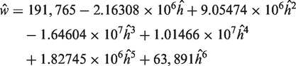
Cantilever test: (a) equilibrium shape for ŵ = 5; (b) weight parameter ŵ versus nondimensional height ĥ. The solid curve is polynomial approximation, and the dashed curve is based on Peirce’s formula.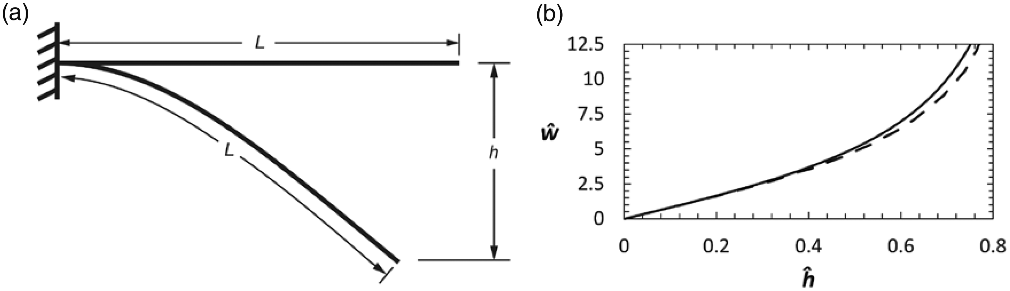

In the following sections, the method will be described and new polynomials will be derived for the different tests (except the free fold test). Then the effective bending rigidity and bending length of the fabric strip can be computed directly from these polynomial formulas.

Method

It is assumed in the analysis that the frictional couple (frictional moment, coercive couple)^23,24 and extensibility¹⁸ have a negligible effect on the fabric shapes under consideration. Friction, hysteresis, and viscoelastic behavior are beyond the scope of the present study. The tests involve uni-directional bending.²⁵ It is assumed that changes across the width of the strip (e.g., anticlastic curvature) are negligible, so that a planar analysis is appropriate. Also, it is assumed that the strip is unstrained when straight (e.g., not curled initially), and that the bending moment is proportional to the curvature, so the model is that of an inextensible elastica.^{8,10–12,26–35}

It is convenient to perform the analysis and present the results in nondimensional form. The nondimensional weight parameter ŵ (which is essentially a weight-to-stiffness ratio²⁹), nondimensional height ĥ, and nondimensional separation â are defined by

\overset{\land}{w} = \frac{{wL}^{3}}{Bb}, \overset{\land}{h} = \frac{h}{L}, \overset{\land}{a} = \frac{a}{L}

(1)

where h is the dimensional height to be measured, and a is the dimensional horizontal separation between the clamped ends of the strip in some of the tests. Following a test and computation of ŵ, the dimensional bending rigidity B and bending length c are found from

B = \frac{{wL}^{3}}{b \overset{\land}{w}}, c = \frac{L}{{\overset{\land}{w}}^{1 / 3}}

(2)

In terms of only dimensional quantities and not involving the length L, one can write c = (Bb/w)^1/3. These formulas are applicable for all the tests in this study.

If the strip has specific weight ρg and a rectangular cross-section with thickness t, then w = ρgbt and B = Et³/12. From Equation (1), ŵ = 12ρgL³/(Et²), and hence the weight parameter ŵ increases if the specific weight ρg increases, the length L increases, the modulus of elasticity E decreases, or the thickness t decreases.

The bending moment M is assumed to be proportional to the curvature K at each deformed location along the strip, with

M = BbK

(3)

Numerical solutions to the governing differential equations and associated boundary conditions are obtained using a shooting method^{29,31–33,35} with the subroutines NDSolve and FindRoot in Mathematica. Then the subroutine NonlinearModelFit is applied to fit these numerical results from the elastica analysis with a polynomial for ŵ(ĥ). (There is one exception, the free fold test, in which a simple formula for ŵ(ĥ) exists.) The approximating polynomials give values of ŵ with less than 0.7% error, except when ŵ is close to zero and the percentage error is not meaningful.

The polynomials are between third and sixth order, with coefficients having between four and nine significant digits, to obtain good accuracy in the approximation over a range of ŵ. (It is noted that Takatera and Shinohara³ developed cubic polynomial approximations equivalent to [ŵ(ĥ)]^1/3 for the cantilever test over the range 1.7 < ŵ < 15.6 and for the heart loop, hanging pear loop, and hanging ring tests over the range 8 < ŵ < 216.) With a calculator or computer, application of these formulas presents no problem. It is not required that measurements of w, L, b, and h have more than two or three significant digits. One can measure h with a ruler, or utilize a digital camera and image processing.^4,9,19

The tests that are investigated in the following sections are the cantilever, heart loop, hanging pear loop, hanging ring, free fold, clamped fold, standing wrinkle (buckle), hanging wrinkle, and standing ring tests. The clamped fold, hanging wrinkle, and standing ring tests have not been applied previously to determine fabric bending rigidity or bending length. Different tests are appropriate for different types of fabric (e.g., stiff or limp^1,5,25). For example, the cantilever test is not well-suited for limp fabrics, so the bending rigidity B should be relatively high and hence ŵ should be relatively low for that test. The approximating polynomials are fit to the data over ranges of ŵ that are suitable for the particular test. The ranges start at ŵ = 0 and end at the following values: ŵ = 16 for the cantilever test, 1000 for the heart loop test, 2500 for the hanging pear loop test, 1000 for the hanging ring test, 368 for the clamped fold test, 500 for the standing wrinkle test, 2200 for the hanging wrinkle test, and 1300 for the standing ring test.

Unlike some of the standard techniques to determine bending rigidity and bending length,^{5,17,18,20,21,36–43} no special equipment is needed for the tests considered here. The fabric strips are only subjected to their self-weight (and are sometimes termed “heavy”^{11,26–28,32,33,44}). Some of the tests only involve curvature with one sense (sign), while equilibrium shapes in other tests involve inflection points and changes in the sense of the curvature.

No experiments were conducted in this study. However, the elastica analysis employed here has previously been verified experimentally for some of the tests. The material does not need to be a fabric. Some of the experiments will be mentioned.

Lammens et al.² used strips of Upilex-50S polyimide foil to compare the theoretical modulus of elasticity found for the cantilever test to that from a tensile test. Differences of 5% and 12% were reported.

For the heart loop test, experiments by Takatera and Shinohara³ included strips made of nylon and of polyester-cotton twill. When the bending rigidity was not too small, its values from the elastica analysis were very close to those from the experiments.

For the hanging pear loop test, Santillan et al.³² showed that the fundamental vibration frequency determined from an elastica analysis was similar to that from experiments using a polycarbonate strip.

For the standing ring test, and for the hanging ring test but with a small horizontal clamping length at the top, Plaut and Virgin³⁵ also used a polycarbonate strip and obtained midpoint deflections very close to those from an elastica analysis.

For the free fold test, Mahadevan and Keller⁴⁵ compared the theoretical bending length to that obtained from experiments with paper and plastic strips, and found the percentage differences to be in the range of 2–4%.

Finally, for the standing wrinkle test, in Santillan et al.³³ a comparison of the height of the strip based on the elastica analysis and on experiments with two polycarbonate strips exhibited excellent agreement over a large range of lengths.

Results and discussion

Cantilever test

The cantilever test has been applied extensively to determine the bending rigidity and bending length of fabric. Following the work of Peirce,¹ further analyses include those in Lammens et al.,² Takatera and Shinohara,³ Potluri et al.,⁷ Moghassem,²² Szablewski and Kobza,³¹ Lippmann et al.,⁴⁴ and Grieβer and Taylor.⁴⁶

The cantilever is illustrated in Figure 1(a), with its clamped (fixed) end at the left and its free end at the right. The unstrained shape with length L is depicted by the horizontal line, and the downward deflection due to self-weight has the value h at the tip. The deformed shape in Figure 1(a) corresponds to the case ĥ = 0.496, with ŵ = 5 and c = 0.585L.

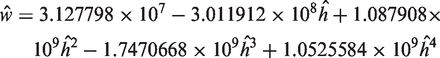
In Figure 1(b), the weight parameter ŵ is plotted as a function of the nondimensional tip deflection ĥ. Here and in subsequent graphs, a solid curve represents the polynomial ŵ(ĥ) computed to fit the theoretical results, and the difference between this polynomial curve and the curve from the elastica analysis would be indistinguishable. The solid curve in Figure 1(b) is the quintic polynomial

\overset{\land}{w} = - 0.025948 + 10.2934 \overset{\land}{h} - 28.8072 {\overset{\land}{h}}^{2} + 134.383 {\overset{\land}{h}}^{3} - 236.785 {\overset{\land}{h}}^{4} + 164.894 {\overset{\land}{h}}^{5}

(4)

and is based on numerical (elastica) results over the range 0 ≤ ĥ ≤ 0.80, with 0 ≤ ŵ ≤ 16 and c ≥ 0.40L. After measuring the tip deflection h in a test, the bending rigidity and bending length are obtained with the use of Equations (2) and (4) if ĥ lies in the given range. (The formula will also be quite accurate over some extension of this range.)

The dashed curves in Figures 1(b), 2(b), 3(b), and 4(b) are obtained from formulas in Peirce¹ (which are repeated in Saville³⁸). Those formulas give the bending length c in terms of an angle θ, which for the cantilever is the angle between the horizontal and the chord connecting the clamped end to the tip. This angle can be computed in the elastica analysis. The standard cantilever case of θ = 41.5° used in the Shirley Stiffness Tester and the FAST-2 Bending Meter^5,6,25,36 corresponds to ŵ = 8, with ĥ = 0.641 and c = L/2. It is seen in Figure 1(b) that, for the cantilever test, the Peirce approximation for ŵ is low, and hence the predictions of the effective bending rigidity B and effective bending length c based on Peirce’s formula are high.^2,3

Figure 2.

Heart loop test: (a) equilibrium shape for ŵ = 500; (b) weight parameter ŵ versus nondimensional height ĥ.

Figure 3.

Hanging pear loop test: (a) equilibrium shape for ŵ = 100; (b) weight parameter ŵ versus nondimensional height ĥ.

Figure 4.

Hanging ring test: (a) equilibrium shape for ŵ = 500; (b) weight parameter ŵ versus nondimensional height ĥ.

Heart loop test

The heart loop is depicted in Figure 2(a). The ends of the strip are clamped together and upward with a vertical tangent, and the height h is the vertical distance from the clamp to the bottom of the loop. The total arc length of the loop from one end to the other is L, and the shape in Figure 2(a) corresponds to ĥ = 0.294, ŵ = 500, and c = 0.126L. Previous studies of the heart loop test include Peirce,¹ Takatera and Shinohara,³ Bickley,²⁶ Lippmann et al.,⁴⁴ and Zhou and Ghosh.⁴⁷

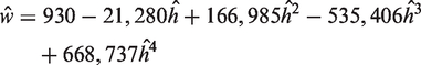
The results are shown in Figure 2(b), based on the elastica analysis in the range 0.133860 ≤ ĥ ≤ 0.349, 0 ≤ ŵ ≤ 1000, and c ≥ 0.1L. These results are fit with the quartic polynomial (solid curve):

\overset{\land}{w} = 930 - 21, 280 \overset{\land}{h} + 166, 985 {\overset{\land}{h}}^{2} - 535, 406 {\overset{\land}{h}}^{3} + 668, 737 {\overset{\land}{h}}^{4}

(5)

Again the Peirce formula (leading to the dashed curve) provides an underestimation of ŵ and an overestimation of B and c.

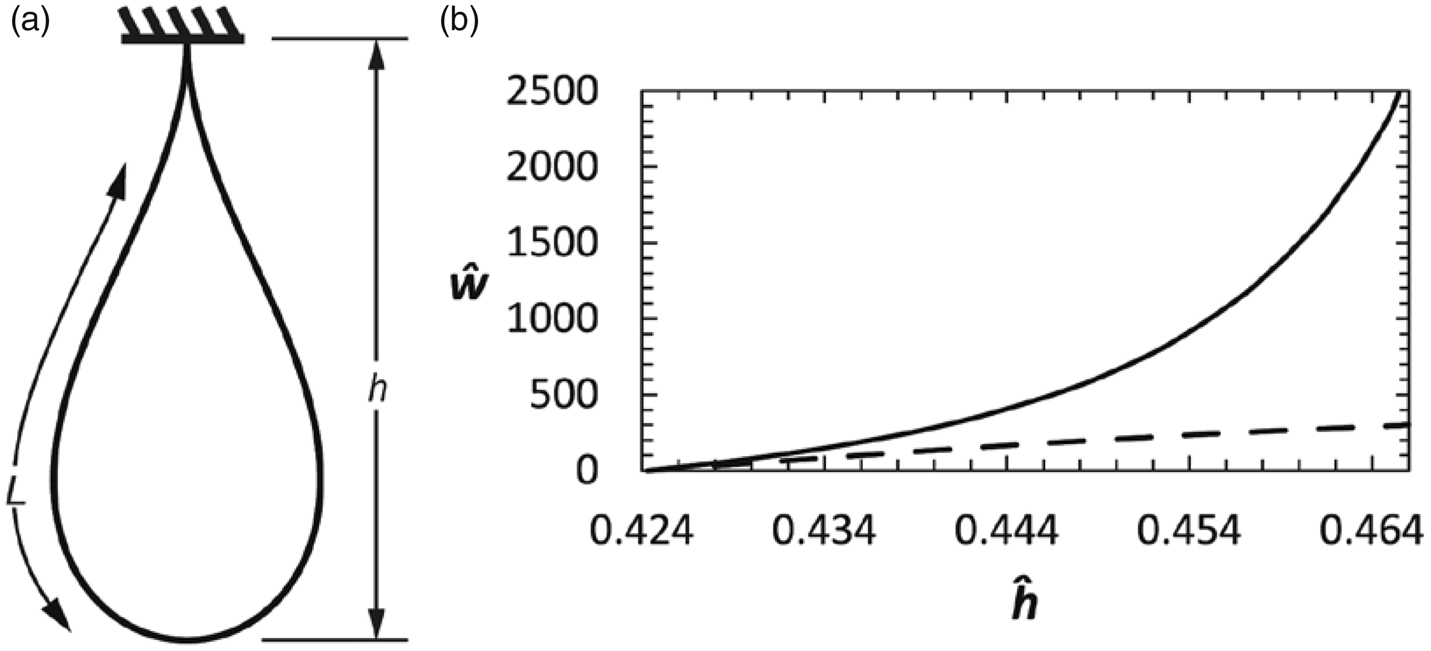
Hanging pear loop test

Figure 3(a) shows the hanging pear loop, with the strip ends clamped together and vertically downward at the top of the loop. The total arc length is L. For this particular shape, ĥ = 0.431, ŵ = 100, and c = 0.215L. Previous analyses include Peirce¹ and Takatera and Shinohara.³ In addition, Naujokaitytė and Strazdienė⁴⁸ investigated a fabric test in which the hanging pear loop is compressed from below by a rigid horizontal plate.

The solution procedure is described in detail by Santillan et al.³² The numerical results for the hanging pear loop lie in the range 0.424308 ≤ ĥ ≤ 0.466, 0 ≤ ŵ ≤ 2,500, and c ≥ 0.074L. Thus, the range of heights in the figure is fairly small. The solid curve in Figure 3(b) is a quintic polynomial given by

\overset{\land}{w} = - 8.3330631 \times 10^{8} + 9.50206993 \times 10^{9} \overset{\land}{h} - 4.33422998 \times 10^{10} {\overset{\land}{h}}^{2} + 9.88557465 \times 10^{10} {\overset{\land}{h}}^{3} - 1.12744452 \times 10^{11} {\overset{\land}{h}}^{4} + 5.143869 \times 10^{10} {\overset{\land}{h}}^{5}

(6)

As pointed out by Takatera and Shinohara,³ the result from Peirce’s formula (dashed curve) is not close except for very small values of the weight parameter.

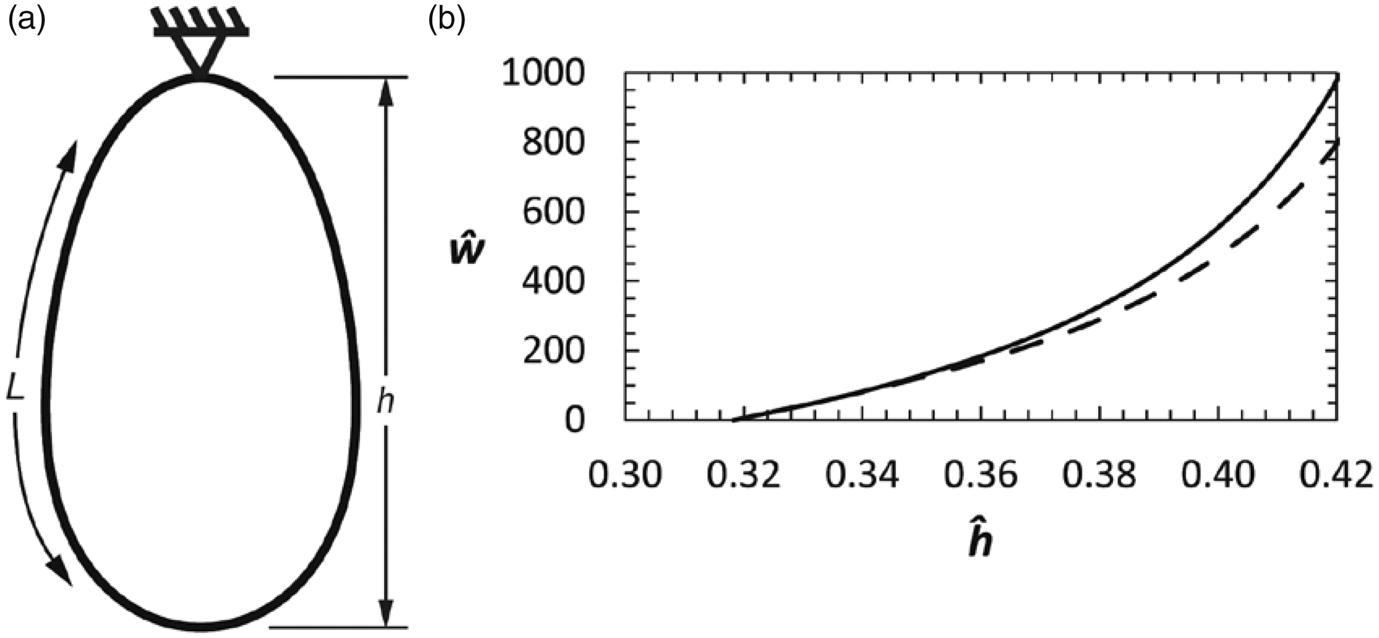
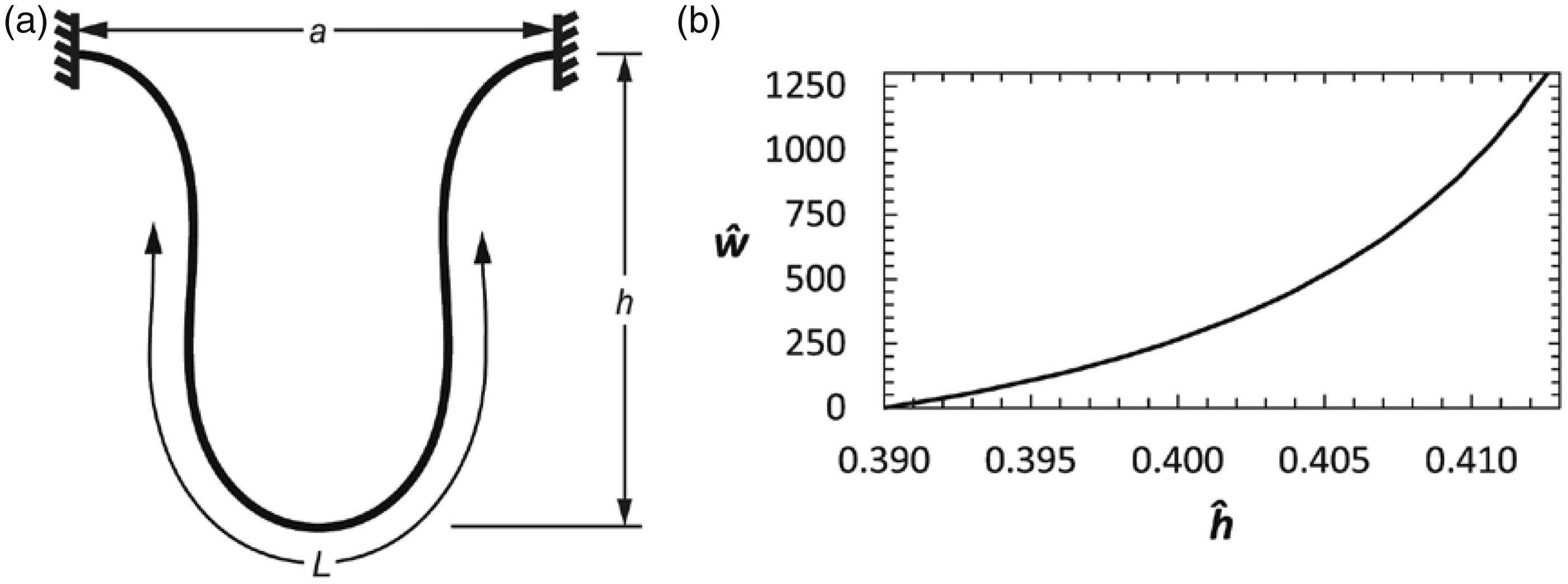
Hanging ring test

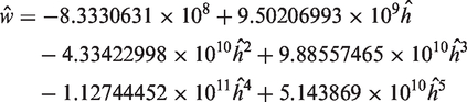
In this test, the loop is supported at its top point and hangs due to self-weight, as illustrated in Figure 4(a) for the case ĥ = 0.396, ŵ = 500, and c = 0.126L. The total arc length is L. The elastica analysis was previously applied by Takatera and Shinohara,³ Watson and Wang,¹⁰ and Plaut and Virgin³⁵ (where the solution procedure is described in detail). In Figure 4(b), the numerical analysis covers the range 0.318309 ≤ ĥ ≤ 0.42, 0 ≤ ŵ ≤ 1,000, and c ≥ 0.1L. The numerical results are fit with the sixth-order polynomial:

\overset{\land}{w} = 191, 765 - 2.16308 \times 10^{6} \overset{\land}{h} + 9.05474 \times 10^{6} {\overset{\land}{h}}^{2} - 1.64604 \times 10^{7} {\overset{\land}{h}}^{3} + 1.01466 \times 10^{7} {\overset{\land}{h}}^{4} + 1.82745 \times 10^{6} {\overset{\land}{h}}^{5} + 63, 891 {\overset{\land}{h}}^{6}

(7)

If ĥ > 0.338, the dashed curve from Peirce’s formula predicts higher values of bending rigidity and bending length than the elastica analysis.

Free fold test

This test was introduced by Stuart⁸ and Stuart and Baird.⁴⁹ It was examined further by others, including Lloyd et al.,²⁷ Wang,²⁸ Mahadevan and Keller,⁴⁵ and Zhou and Ghosh.⁴⁷ It is called the “free fold test” in this section to distinguish it from the “clamped fold test” in the following section. (A related test was proposed by Cassidy et al.²⁵) Here a long strip rests on a rigid horizontal surface and is folded back onto itself. It forms a loop, and on the left of the loop in Figure 5(a) the two end segments of the strip (with arbitrary lengths) are horizontal. (The arc length L in the figure does not include these end segments.) In the analysis, the thickness of the strip is neglected in the boundary conditions at the point where the top segment lifts off the bottom segment at the left end of the loop.

Figure 5.

Free fold test: (a) equilibrium shape for ŵ = 368; (b) weight parameter ŵ versus nondimensional height ĥ – the solid curve denotes the analytical solution in this case only.

Figure 5(a) depicts the shape for ĥ = 0.127, ŵ = 368, and c = 0.140L. This test is different from the others considered in this paper, in that there is a simple relationship between the parameters ĥ and ŵ.^8,28 It is given by

\overset{\land}{w} = \frac{0.74515}{{\overset{\land}{h}}^{3}}

(8)

Equation (8) is applicable for any value of ĥ, and is plotted in Figure 5(b) for 0 ≤ ŵ ≤ 2000.

In dimensional terms, Equations (1), (2), and (8) lead to

B = 1.342 \frac{{wh}^{3}}{b}, c = 1.103 h

(9)

which do not involve L. The bending rigidity and bending length can be determined directly from Equation (9).

For this free fold test to be possible, the dimensional length of the strip must be longer than 4.683(Bb/w)^1/3, that is, 4.683c (Wang²⁸). For this minimum length, the strip only includes the uplifted part in Figure 5(a). The length L does not appear in Equation (9) and does not have to be measured.

Clamped fold test

The new test in this section is the same as the free fold test except that the ends of the strip are clamped together, as shown in Figure 6(a). The shape in Figure 6(a) corresponds to ĥ = 0.171, ŵ = 100, and c = 0.215L, where L is the total arc length of the strip. If ŵ is increased to 368 (with ĥ = 0.127), the shape becomes the loop in Figure 5(a). If ŵ > 368 (with ĥ < 0.127), the top and bottom parts of the strip near the clamped end rest on the horizontal surface, and then Equations (8) and (9) are applicable. Therefore, only ŵ ≤ 368 needs to be considered in this section.

Figure 6.

Clamped fold test: (a) equilibrium shape for ŵ = 100; (b) weight parameter ŵ versus nondimensional height ĥ.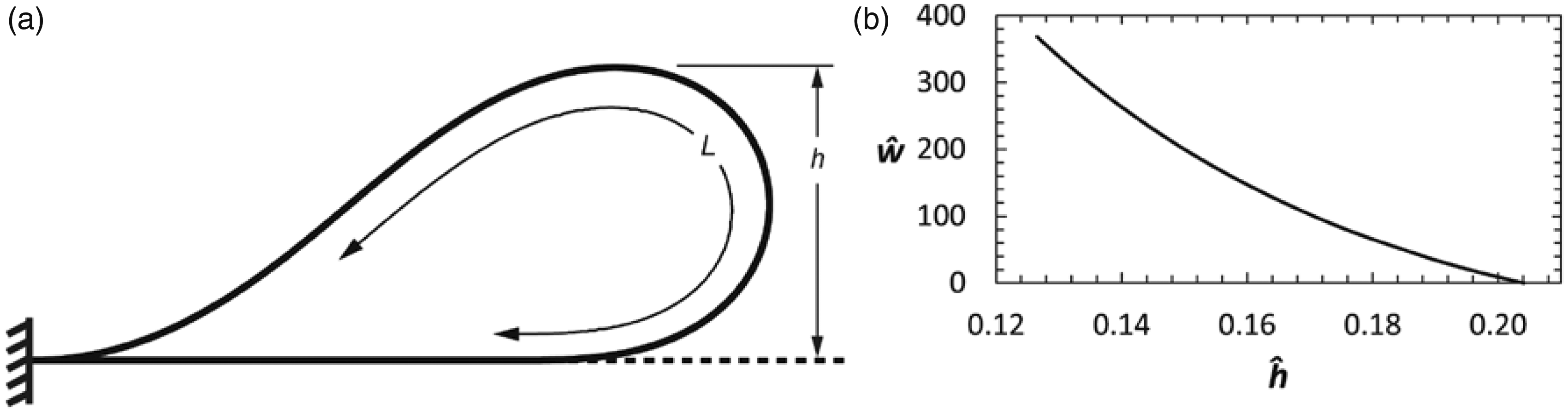

The numerical results from the elastica analysis range from ĥ = 0.204091 (for ŵ = 0) to ĥ = 0.127 (for ŵ = 368). They are fit with the cubic equation

\overset{\land}{w} = 2, 963 - 35, 969 \overset{\land}{h} + 149, 972 {\overset{\land}{h}}^{2} - 219, 888 {\overset{\land}{h}}^{3}

(10)

shown in Figure 6(b). In this range, with 0 ≤ ŵ ≤ 368 and c ≥ 0.140L, the values of B and c are obtained from Equations (2) and (10).

Standing wrinkle test

For this test, the fabric strip lies on or above a horizontal surface. The ends of the strip are clamped with a horizontal separation a. The nondimensional length is â = a/L, where L is the total arc length of the strip between the clamped ends. In this section, it is arbitrarily assumed that L = 2a, that is, â = 0.5. The equilibrium shapes in Figures 7(a) and 7(b) correspond, respectively, to ĥ = 0.366 (with ŵ = 100 and c = 0.215L) and ĥ = 0.289 (with ŵ = 500 and c = 0.126L). In Figure 7(b), the nondimensional contact length of the strip with the horizontal surface is 0.095 adjacent to each clamped end.

Figure 7.

Standing wrinkle test with a = 0.5L: equilibrium shapes for (a) ŵ = 100 and (b) ŵ = 500; (c) weight parameter ŵ versus nondimensional height ĥ.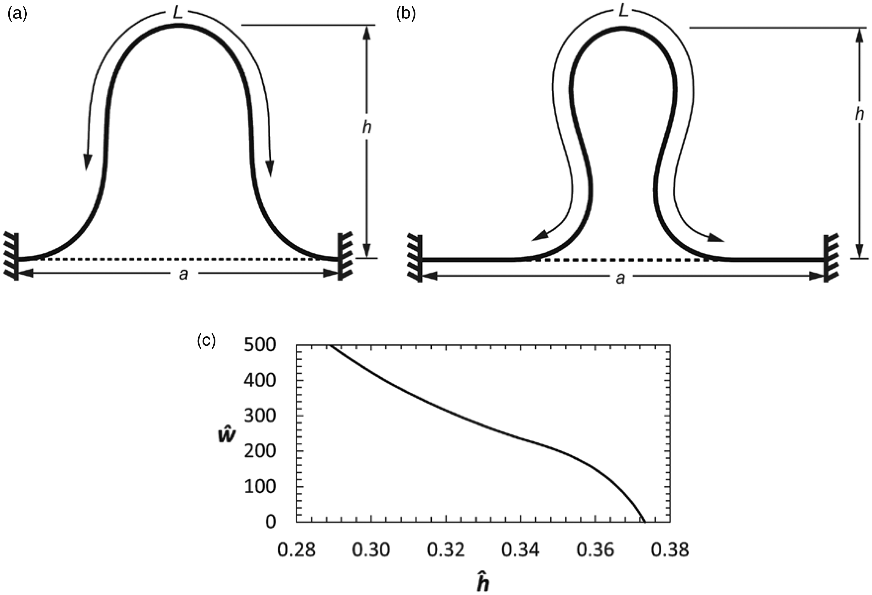

This type of problem is usually discussed with respect to buckling, and most attention has been focused on the relationship between the compressive load and the distance between the ends of the wrinkle (buckle).^{12,15,19,29,34,50–52} (Theoretically, if a heavy elastic strip with finite length L rests on a rigid horizontal surface, it cannot be buckled by any finite, horizontal, compressive load applied at its ends.¹²) Wang¹² calls the configuration “long” if the strip has end segments resting on the surface (as in Figure 7(b)) and “short” if it does not (as in Figure 7(a)).

Jakubčionienė et al.⁵³ considered a fabric configuration similar to that in Figure 7(a), with a specific separation between the clamped ends. However, their test involved compression by a rigid horizontal plate that moved downward onto the wrinkle. Here the relationship between the self-weight and the height of the wrinkle is examined.

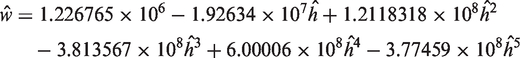
The solution procedure is described in detail by Santillan et al.³³ Results are plotted in Figure 7(c). When the self-weight is zero, ĥ = 0.373306. The equilibrium shape is short until ŵ = 223, for which ĥ = 0.344. The numerical results in Figure 7(c) end at ŵ = 500, with ĥ = 0.289 (shape in Figure 7(b)). The quintic polynomial used to fit the results from the elastica analysis over the range 0 ≤ ŵ ≤ 500 is

\overset{\land}{w} = 1.226765 \times 10^{6} - 1.92634 \times 10^{7} \overset{\land}{h} + 1.2118318 \times 10^{8} {\overset{\land}{h}}^{2} - 3.813567 \times 10^{8} {\overset{\land}{h}}^{3} + 6.00006 \times 10^{8} {\overset{\land}{h}}^{4} - 3.77459 \times 10^{8} {\overset{\land}{h}}^{5}

(11)

This formula can be applied with different dimensional separations a between the clamped ends if the strip length L between the clamped ends is 2a.

Hanging wrinkle test

For this new fabric test, the wrinkle hangs downward between the clamped ends. The total arc length is L. Two cases are arbitrarily selected: L = 5a, that is, â = 0.2 (Figure 8), and L = 2.5a, that is, â = 0.4 (Figure 9). An elastica analysis was presented by Watson and Wang.¹¹ A related configuration was studied by Zhou and Ghosh,⁴⁷ where the ends of the strip were not clamped, but rested on circular rollers. Also, Jakubčionienė et al.⁵³ and Masteikaitė et al.⁵⁴ investigated a test in which a hanging wrinkle was compressed by an upward-moving rigid horizontal plate.

Figure 8.

Hanging wrinkle test with a = 0.2L: (a) equilibrium shape for ŵ = 100; (b) weight parameter ŵ versus nondimensional height ĥ.

Figure 9.

Hanging wrinkle test with a = 0.4L: (a) equilibrium shape for ŵ = 100; (b) weight parameter ŵ versus nondimensional height ĥ.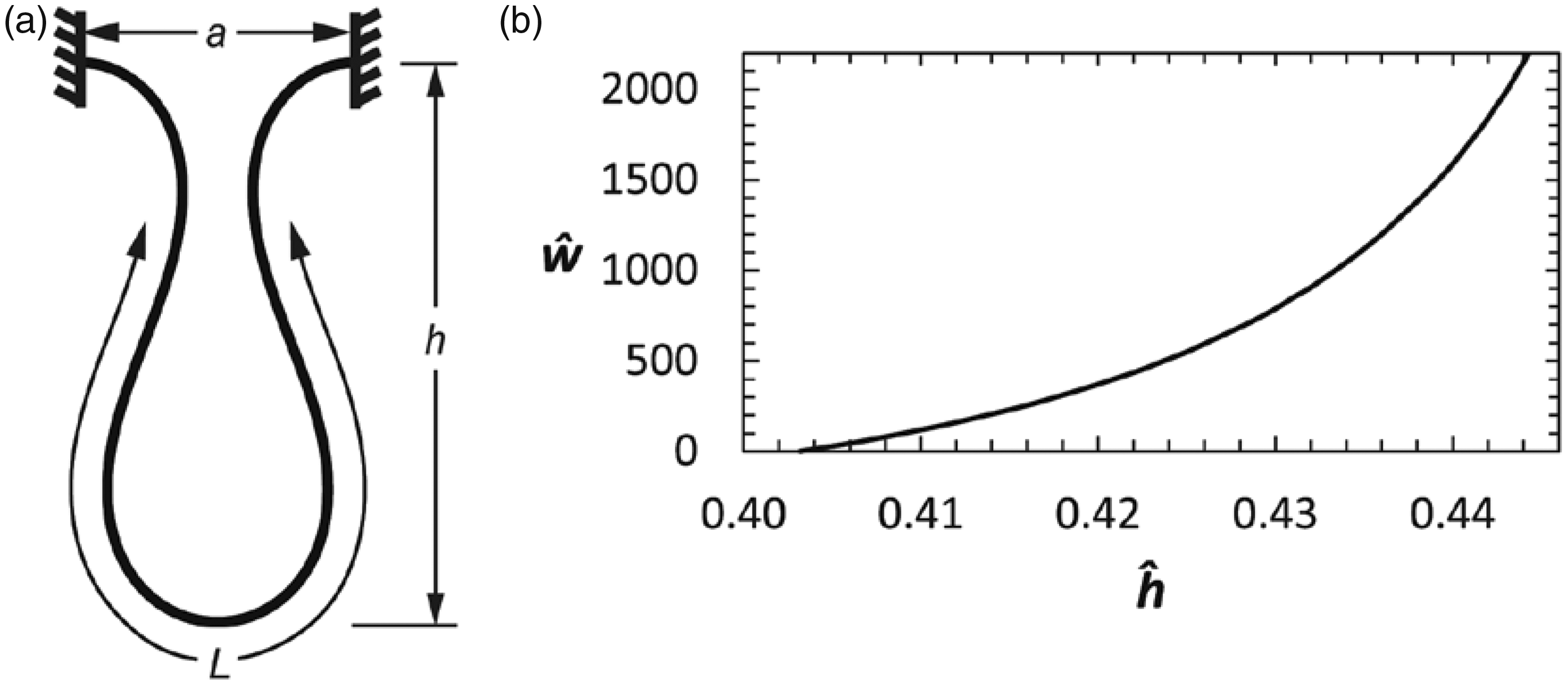

First consider the case â = 0.2. The equilibrium shape in Figure 8(a) corresponds to ĥ = 0.409, with ŵ = 100 and c = 0.215L. The elastica analysis yields ĥ = 0.403132 for ŵ = 0 and, at the end of the range in Figure 8(b), ĥ = 0.444 for ŵ = 2200 (where c = 0.077L). The approximating quartic polynomial for this range is

\overset{\land}{w} = 3.127798 \times 10^{7} - 3.011912 \times 10^{8} \overset{\land}{h} + 1.087908 \times 10^{9} {\overset{\land}{h}}^{2} - 1.7470668 \times 10^{9} {\overset{\land}{h}}^{3} + 1.0525584 \times 10^{9} {\overset{\land}{h}}^{4}

(12)

For the case â = 0.4, Figure 9(a) also corresponds to ŵ = 100 and c = 0.215L, but now ĥ = 0.395. In Figure 9(b), ĥ = 0.389972 for ŵ = 0, and ĥ = 0.413 for ŵ = 1300 (where c = 0.092L). The elastica results for this range are fit with the quartic polynomial

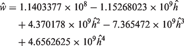
\overset{\land}{w} = 1.1403377 \times 10^{8} - 1.15268023 \times 10^{9} \overset{\land}{h} + 4.370178 \times 10^{9} {\overset{\land}{h}}^{2} - 7.365472 \times 10^{9} {\overset{\land}{h}}^{3} + 4.6562625 \times 10^{9} {\overset{\land}{h}}^{4}

(13)

Standing ring test

Another new test is considered in this section. A ring (loop) with circumference L rests on a rigid horizontal surface. For fabrics, Stuart et al.³⁰ considered such a ring subjected to downward compression by a rigid horizontal plate, and neglected the ring’s weight in the analysis. For the heavy ring of interest, Plaut and Virgin³⁵ and Wang and Watson⁵⁵ applied the elastica model to determine equilibrium configurations. The solution procedure used here is described in detail by Plaut and Virgin.³⁵

In this section, the symbol h denotes the height of the midpoint of the top part of the ring, and ĥ = h/L as before. For the equilibrium shape in Figure 10(a), ŵ = 500 (with c = 0.126L) and ĥ = 0.163. In Figure 10(b), ŵ = 1000 (with c = 0.1L), ĥ = 0.084, and the maximum height (with nondimensional value 0.103) is not at the midpoint. The nondimensional contact length of the ring with the horizontal surface is 0.203 in Figure 10(a) and 0.287 in Figure 10(b).

Figure 10.

Standing ring test: equilibrium shapes for (a) ŵ = 500 and (b) ŵ = 1,000; (c) weight parameter ŵ versus nondimensional height ĥ.

It is noted that the ring’s equilibrium shape is circular when ŵ = 0, with ĥ = 1/π = 0.3183. As ŵ is increased, the contact length of the ring with the surface remains zero until ŵ = 147 (with ĥ = 0.262 and c = 0.189L), the curvature at the midpoint of the top part of the loop changes sign when ŵ = 564 (with ĥ = 0.151 and c = 0.121L), and ĥ becomes zero when ŵ reaches 1409 (with c = 0.089L).

The curve in Figure 10(c) is based on numerical results ranging from ŵ = 0 to ŵ = 1409. The formula for this approximating curve is the quartic polynomial

\overset{\land}{w} = 1, 408 - 1, 904 \overset{\land}{h} - 56, 660 {\overset{\land}{h}}^{2} + 268, 555 {\overset{\land}{h}}^{3} - 361, 752 {\overset{\land}{h}}^{4}

(14)

Concluding remarks

This study has considered some standard tests and some new tests of fabrics in order to determine an effective bending rigidity B and an effective bending length c. The tests do not require any special equipment or applied loads. The results are based on measurement of a vertical deflection of the equilibrium shape of a fabric strip. The only other required measurements are the length, width, and weight of the strip. The inextensible-elastica theory used in many previous related studies was applied in nondimensional form, and polynomials were derived that enable B and c to be computed in a simple manner.

The approximating polynomials give values of the weight parameter ŵ with less than 0.7% error, except when ŵ is close to zero and the percentage error is not meaningful. The polynomials are between third and sixth order, with coefficients having between four and nine significant digits, to obtain good accuracy in the approximation over a range of ŵ. However, it is not required that measurements of the weight, length, width, and height have more than two or three significant digits.

The tests can be conducted with various strip lengths to model shapes that are relevant for particular applications. The strips can be constructed in the weft, warp, or bias directions to investigate the directionality effect. The orientation of the strip can be changed, by turning it upside down or inside out, to see how the bending rigidity B and the bending length c are affected.

In conclusion, it is hoped that the present study will be useful to the textile industry, providing an alternative to formulas and techniques already available.

Footnotes

Funding

This research received no specific grant from any funding agency in the public, commercial, or not-for-profit sectors.

Acknowledgments

The author is grateful to Benjamin Z Dymond for preparing the figures, and to the five reviewers for their helpful suggestions.

References

Peirce

. The “handle” of cloth as a measurable quantity. J Textil Inst Trans 1930; 21: T377–T416.

Lammens

Kersemans

Luyckx

. Improved accuracy in the determination of flexural rigidity of textile fabrics by the Peirce cantilever test (ASTM D1388). Textil Res J 2014; 84: 1307–1314.

Takatera

Shinohara

. A unified analysis to compare conventional methods for estimating bending rigidity of fabrics. J Textil Mach Soc Jpn 1996; 42: 86–92.

Clapp

Peng

Ghosh

. Indirect measurement of the moment-curvature relationship for fabrics. Textil Res J 1990; 60: 525–533.

Ghosh

Zhou

. Characterization of fabric bending behavior: a review of measurement principles. Indian J Fibre Textil Res 2003; 28: 471–476.

Sun

. A new tester and method for measuring fabric stiffness and drape. Textil Res J 2008; 78: 761–770.

Potluri

Atkinson

Porat

. Large deformation modelling of flexible materials. J Textil Inst 1996; 87: 129–151.

Stuart

. A loop test for bending length and rigidity. Brit J Appl Phys 1966; 17: 1215–1220.

Ghane

Hedayati

. A fixed-supported beam modelling for measuring fabric rigidity using small deflection equations. J Textil Inst 2014; 105: 93–99.

10.

Watson

Wang

. Hanging an elastic ring. Int J Mech Sci 1981; 23: 161–167.

11.

Watson

Wang

. Periodically supported heavy elastic sheet. J Eng Mech 1983; 109: 811–820.

12.

Wang

. On symmetric buckling of a finite flat-lying heavy sheet. J Appl Mech 1984; 51: 278–282.

13.

Clapp

Peng

. A comparison of linear and non-linear bending models for predicting fabric deformation in automated handling. J Textil Inst 1991; 82: 341–352.

14.

Zhou

Ghosh

. On-line measurement of fabric bending behavior, Part II: Effects of fabric nonlinear bending behavior. Textil Res J 1998; 68: 533–542.

15.

Kang

Joo

Lee

. Analyzing fabric buckling based on nonlinear bending properties. Textil Res J 2004; 74: 172–177.

16.

Szablewski

. Numerical identification of elasticity coefficients for the bending problem. AUTEX Res J 2004; 4: 206–210.

17.

Zhou

Yan

. Measurement and characterization of bending stiffness for fabrics. Fibers Polym 2011; 12: 104–110.

18.

. Structure and mechanics of woven fabrics, Cambridge: Woodhead, 2004.

19.

Domskienė

Strazdienė

. The effect of bending rigidity upon fabric behaviour under in-plane compression. Tekstil 2005; 54: 260–265.

20.

Naujokaitytė

Strazdienė

Fridrichová

. Comparative analysis of fabrics’ bending behavior testing methods. Tekstil 2007; 56: 343–349.

21.

Ancutienė

Strazdienė

Nesterova

. The relationship between fabrics bending rigidity parameters defined by KES-F and FAST equipment. Mater Sci (Medžiagotyra) 2010; 16: 346–352.

22.

Moghassem

. A new approach for numerical identification of bending behavior of plain woven fabric. Fibers Polym 2012; 13: 237–243.

23.

Clapp

Peng

. Buckling of woven fabrics, Part II: Effect of weight and frictional couple. Textil Res J 1990; 60: 285–292.

24.

Ghosh

Batra

Barker

. The bending behaviour of plain-woven fabrics, Part I: A critical review. J Textil Inst 1990; 81: 245–254.

25.

Cassidy

Cassie

. The stiffness of knitted fabrics: a new approach to the measurement of bending - Part 1: Development. Int J Cloth Sci Technol 1991; 3: 14–19.

26.

Bickley

. The heavy elastica. Phil Mag 1934; 17: 603–622.

27.

Lloyd

Shanahan

Konopasek

. The folding of heavy fabric sheets. Int J Mech Sci 1978; 20: 521–527.

28.

Wang

. Post-buckling of horizontal heavy elastic sheet. J Eng Mech 1984; 110: 871–878.

29.

Clapp

Peng

. Buckling of woven fabrics, Part I: Effect of fabric weight. Textil Res J 1990; 60: 228–234.

30.

Stuart

Hetherington

Baird

. An investigation of cloth bending, Part I: Compression of looped fabrics. Textil Res J 1966; 36: 803–808.

31.

Szablewski

Kobza

. Numerical analysis of Peirce’s cantilever test for the bending rigidity of textiles. Fibres Textil East Eur 2003; 11: 54–57.

32.

Santillan

Virgin

Plaut

. Equilibria and vibration of a heavy pinched loop. J Sound Vib 2005; 288: 81–90.

33.

Santillan

Virgin

Plaut

. Post-buckling and vibration of heavy beam on horizontal or inclined rigid foundation. J Appl Mech 2006; 73: 664–671.

34.

Wagner

TJW

Vella

. The ‘sticky elastica’: delamination blisters beyond small deformations. Soft Matter 2013; 9: 1025–1030.

35.

Plaut

Virgin

. Deformation and vibration of upright loops on a foundation and of hanging loops. Int J Solids Struc 2014; 51: 3067–3075.

36.

Tester

Buckenham

. Simple instruments for quality control by finishers and tailors. Textil Res J 1991; 61: 402–406.

37.

Zhou

Ghosh

. On-line measurement of fabric-bending behaviour: background, need and potential solutions. Int J Cloth Sci Technol 1998; 10: 143–156.

38.

Saville

. Physical testing of textiles, Cambridge: Woodhead, 1999.

39.

De Boos

Concepts and understanding of fabric hand. In: Behery

(ed). Effect of mechanical and physical properties on fabric hand, Cambridge: Woodhead, 2005, pp. 11–44.

40.

. Determination of the bending characteristic parameters of the bending evaluation system of fabric and yarn. Textil Res J 2006; 76: 702–711.

41.

Tokmak

Berkalp

Gersak

. Investigation of the mechanics and performance of woven fabrics using objective evaluation techniques, Part I: The relationship between FAST, KES-F and Cusick’s drape-meter parameters. Fibres Textil East Eur 2010; 18: 55–59.

42.

Fridrichová

. A new method of measuring the bending rigidity of fabrics and its application to the determination of their anisotropy. Textil Res J 2013; 83: 883–892.

43.

Goetzendorf-Grabowska

Karaszewska

Vlasenko

. Bending stiffness of knitted fabrics - comparison of test methods. Fibres Textil East Eur 2014; 22: 43–50.

44.

Lippmann

Mahrenholtz

Johnson

. Thin heavy elastic strips at large deflexions. Int J Mech Sci 1961; 2: 294–310.

45.

Mahadevan

Keller

. Periodic folding of thin sheets. SIAM Rev 1999; 41: 115–131.

46.

Grieβer

Taylor

. The bending behaviour of fabrics: an energy approach. Math Comput Simulat 1996; 41: 579–586.

47.

Zhou

Ghosh

. On-line measurement of fabric bending behaviour. Part I: Theoretical study of static fabric loops. Textil Res J 1997; 67: 712–719.

48.

Naujokaitytė

Strazdienė

. Investigation of textile fabrics behaviour under compression. Mater Sci (Medžiagotyra) 2007; 13: 337–342.

49.

Stuart

Baird

. A new test for bending length. Textil Res J 1966; 36: 91–93.

50.

Kopp

Rahn

Paul

. Measuring deformations of limp fabrics for material handling. Textil Res J 2000; 70: 920–932.

51.

Domokos

Fraser

Szeberényi

. Symmetry-breaking bifurcations of the uplifted elastic strip. Physica D 2003; 185: 67–77.

52.

Palmer

Williams

. Frost heave and pipeline upheaval buckling. Can Geotech J 2003; 40: 1033–1038.

53.

Jakubčionienė Ž, Masteikaitė V and Sacevičienė V. New method and device for clothing materials deformation evaluation. In: Mechanika 2010: proceedings of the 15th international conference, Kaunas, Lithuania, 8–9 April, 2010, pp.188–192.

54.

Masteikaitė

Sacevičienė

Čironienė

. Compressed loop method for the bending behaviour of coated and laminated fabrics analysis. J Indus Textil 2014; 43: 350–365.

55.

Wang

Watson

. Equilibrium of heavy cylindrical shells. J Appl Mech 1981; 48: 582–586.