Numerical modeling of the air permeability of two-layer woven structure ensembles

Abstract

This study aims at investigating air permeability in the transversal direction of pairs of woven textiles. Three samples of woven macrostructures with different characteristics are selected for the numerical investigation of 16 two-layer ensembles. Computational fluid dynamics (Reynolds-averaged Navier–Stokes equations) is used for modeling the air permeability, applying the theory of jet-systems: the flow through each of the layers in the ensemble is modeled as an “in-corridor” ordered jet-system. The influence of the order of arrangement of the layers in the ensemble is analyzed, indicating higher air permeability of the ensemble when a tighter structure is placed as a first layer. The effect of the distance between the two woven macrostructures is also analyzed, showing a strong influence on the flow development as well as on the extrema of flow velocities, especially in the drop of the flow velocity in the air gap between the two layers. The analysis made and the results obtained show that the method can be applied for further investigation of ensembles of textile layers.

Keywords

air permeability two-layer ensembles numerical simulation computational fluid dynamics jet systems woven structures

The thermophysiological comfort of human beings is strongly dependent on clothing, influenced, in turns, by fabric properties: air permeability (AP), heat transfer, water vapor permeability, etc.¹ The AP of textiles is an important feature, as it is responsible for transport of air and water vapor from the body to the surrounding environment.² It is determined as the flow rate in the transversal direction of a textile macrostructure, measured when a pressure gradient between the two surfaces of the sample exists. However, the proper simulation of the AP of a textile macrostructures would allow the prediction of this characteristic at the design stage, reducing expenses for production of samples with different properties.

Several research studies have been dedicated to the problems of AP simulation. Kulichenko and Langenhove³ used the formula of Hagen–Poiseuille together with the D’Arcy law, in order to derive an equation for the theoretical analysis of the relationship between the AP and the textile structure. Xu and Wang⁴ applied the same method, but their research was based on textile macrostructures, made of monofilaments. Belkacemi and Broadbent⁵ were focused on studying the permeability of textiles at high differential pressure gradients, both experimentally and theoretically. The porosity of a single-layer textile was explored by Jakšić and Jakšić,⁶ and a mathematical model of the porosity was developed. Ogulata and Mavruz⁷ also studied the porosity and AP of a single-layer textile by developing a complex mathematical model based on the D’Arcy’s formula. Gibson et al.⁸ focused on the dynamic AP of a porous elastic textile, but they used a real experimental set.

A statistical method was developed by Epps⁹ to describe the relationship between the structure of a textile and its AP. Computational fluid dynamics (CFD) code was used as an instrument by Nazarboland et al.¹⁰ in order to simulate AP based on the thickness of the textile. Grouve et al.¹¹ developed their own CFD code for calculation of the AP of textiles in the transversal direction. Rief et al.¹² studied the AP of textiles by using their own software, based on the multitude of initially preset parameters obtained from real experiments.

Most of the research in the field of AP was mainly based on single-layer textile macrostructures. Elnashar¹³ studied experimentally the AP of double-layer woven fabrics with different constructions of the upper and lower weave. Padaki et al.¹⁴ simulated the resin flow through multilayered textiles with known porosity and permeability by using a CFD model. However, there are hardly any studies on the simulation of AP of two-layer fabric ensembles. In reality, clothing is made of two or more textile layers to maintain the thermophysiological comfort; therefore, it is essential to understand the behavior of ensembles of textiles.

Our previous research has shown the applicability of a method for simulation of the AP of single-layer woven macrostructures, based on the jet system theory.^15,16 The method was tested numerically and verified with experimental results for the AP of real fabrics. The objective of the present study was to investigate numerically the AP of two-layer fabric ensembles. The same method for approximation, based on jet systems was applied, and the FLUENT CFD software package was used for the simulations.

Theory

A jet system can be considered a system in which the air is passing through openings in the solid structure. The interaction between the jets, leaving the openings, forms a complex three-dimensional (3D) flow. The openings can be of various shapes (square, rectangular, circle) and ordered in-line, in-corridor and chess-board.¹⁷

Figure 1 shows an in-corridor arranged jet system of 3 × 3 ordered square openings (nine openings in total), with a unit length of $2 b_{0}$ per opening. Figure 1(a) is a 3D orthogonal representation of the jet system, Figure 1(b) is a two-dimensional (2D) representation with the basic parameters of the jet system, and Figure 1(c) is a transversal representation of the turbulent flow development and dissipation until gradually intermixing from a single jet (region I) into the flow field (region IV). The steps between the openings are characterized by the parameters S_y and S_z, as follows:^16,17

S_{y} = 2 b_{0} + d_{wp} S_{z} = 2 b_{0} + d_{wf}

(1)

where d_wp and d_wf are the average diameter of warp and weft yarns, respectively, mm, and b₀ is the equivalent pore size. The last is calculated as

2 b_{0} = \sqrt{S_{m}}

(2)

where S_m is the mean pore area, mm².

Figure 1.

In-corridor ordered jet system: (a) three-dimensional view; (b) basic metrics; (c) flow development – transversal representation.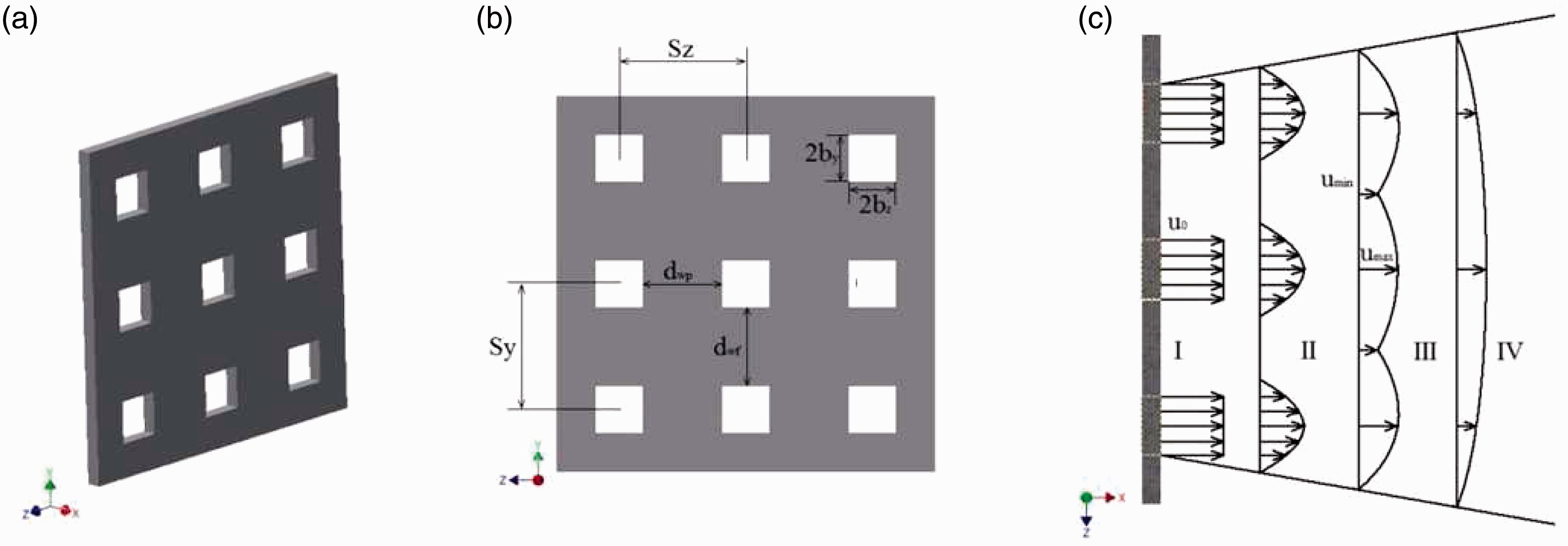

The flow starts with initial velocity of u₀ (Figure 1(c)). The flow of every single pore is independently developing in region I. Between regions II and III, the single flows are beginning to intermix until in section IV they have further developed into one steady-state flow.¹⁷

The woven fabrics have such a specific geometry that they are very similar to a tube-like porous structure. The geometry is defined by the interweaving of the weft and the warp threads with repeated interchanges of the threads and voids in both directions of the weft and warp. This macrostructure is very similar to the in-corridor ordered jet system.

Every single jet in the in-corridor jet system is representative for the whole system, if it is surrounded by eight other jets.¹⁷ The surrounding eight flows are acting as boundary conditions and influence the flow development of the central jet. Thus, every woven macrostructure fabric can be approximated to an in-corridor ordered jet system of nine openings, which means the woven textile is simulated as 4 × 4 yarns or 3 × 3 pores between the yarns.¹⁶ This basic approach was described in detail, applied for simulation of real woven fabrics and verified with experimental results for the AP of woven fabrics in Angelova et al.^15,16 The method was also applied for simulation of the AP of knitted fabrics.¹⁸

A previous numerical study on the problem has shown¹⁵ that there is practically no difference between the circular and square shaped openings in a jet system. Being the case, it is up to the personal preferences and the grid used on whether the used shape will be circular or square. For the purpose of this study a square shape of the pores was chosen.

Materials and methods

Materials

Three samples of woven macrostructures with different geometrical characteristics were selected for creating the pairs of layers for the simulation, as shown in Table 1. All they were made of cotton yarns in a plain weave, with a large difference in the porosity of Sample K and similar porosity of Sample P and Sample Y. The porosity V_s of the samples was determined on the basis of warp P_wa and weft P_wf densities of the samples, as well as their warp E_wa and weft cover factors E_wf, following the equation

V_{s} = 100 - (E_{wa} + E_{wf} - 0.01 E_{wa} E_{wf})

(3)

for

E_{wa} = k_{f} P_{wa} \sqrt{\frac{{Tt}_{wa}}{1000}}, % E_{wf} = k_{f} P_{wf} \sqrt{\frac{{Tt}_{wf}}{1000}}, %

(4)

where Тt_wa is the linear density of the warp threads, tex; Tt_wf is the linear density of the weft threads, tex; and k_f is a coefficient that depends on the fiber type.

Table 1.

Basic characteristics of the simulated woven macrostructures

Sample code	Material	Weave	Weight, g/m²	Warp density, ends/dm	Weft density, picks/dm	Linear density warp, tex	Linear density weft, tex	Thickness, mm	Porosity, %	Mean pore area S_m, mm²
К	CO 100%	Plain	89	176	124	28	28	0.45	51.6	0.255
P	CO 100%	Plain	133	284	294	20	20	0.39	29.1	0.038
Y	CO 100%	Plain	157	234	254	30	30	0.47	25.9	0.031

Due to the complexity of the geometry of each fabric individually, the following simplifications when creating the virtual model of the samples have been assumed.

The diameter of the yarn was accepted to be one and the same along the thread.

The pore area was approximated to an average value for the whole macrostructure S_m (Table 1). The square shape of the pores was used.

As the interweaving of the warp and weft threads had an influence on the thickness, an average value from the experimental measurement of the thickness was accepted as length of the interstices.¹⁹

Every simulated sample was presented as a system of 4 × 4 threads, which interconnection gave an “in-corridor” ordered system of 3 × 3 jet flows (3 × 3 pores). However, as the simulated macrostructures had different values of warp and weft density, in the geometrical models one of the samples had always at least 3 × 3 pores, whereas the other might have a greater number of pores to reach the same sample size.

Figure 2 represents the approach used for modeling of Sample K: the microscopic picture of the woven structure (Figure 2(a)) and the geometry built with FLUENT’s GAMBIT pre-processor (Figure 2(b)), based on a 3 × 3 jet system.

Figure 2.

Approach in modeling of the woven structure: (a) microscopic picture of Sample K; (b) the geometry, built in GAMBIT.

Numerical procedure

The geometry of each pair of woven structures was built using a GAMBIT FLUENT pre-processor. A pipe-like domain was used, where the first layer (woven structure) was placed 3 mm after the domain inlet. The second layer was built in a distance of 0.5 – 1 – 3 – 5 mm from the first one and 8 mm before the domain outlet. The length of the domain had to ensure the flow development after the second layer.¹⁶

Figure 3 shows the domain for Case 1 (Sample K – Sample P at a distance of 0.5 mm) – see Table 2.

Figure 3.

Three-dimensional geometrical model for Case 1.

Table 2.

Simulated cases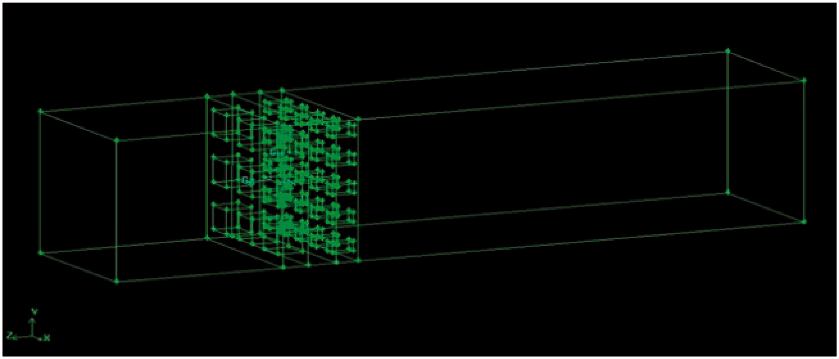

Computational case	First layer	Second layer	Distance between the two layers, mm	Number of cells	Number of faces	Number of nodes
1	K	P	0.5	134,350	391,110	125,501
2	K	P	1	158,761	440,652	130,064
3	K	P	3	254,634	643,918	147,737
4	K	P	5	350,003	828,176	165,324
5	P	K	0.5	128,318	373,014	119,469
6	P	K	1	152,729	422,556	124,032
7	P	K	3	248,602	616,822	141,705
8	P	K	5	343,971	810,080	159,292
9	P	Y	0.5	71,799	211,721	69,636
10	P	Y	1	76,561	221,373	70,473
11	P	Y	3	101,402	272,903	75,870
12	P	Y	5	201,774	476,779	94,899
13	Y	P	0.5	68,103	200,633	65,940
14	Y	P	1	71,689	206,757	65,601
15	Y	P	3	96,530	258,287	70,998
16	Y	P	5	198,582	467,203	91,707

In order for the virtual model of Sample K to include 3 × 3 pores, its size was larger than the size of the Sample K, which has higher values of warp and weft densities (Table 1). Thus, the larger sample size was determinant for the size of the computational domain and the second woven macrostructure in the pair. As a result, Sample P was built with 25 pores (5 × 5).

A hybrid grid of tetrahedrons (between the samples) and hexahedrons (in the rest of the domain) was used for meshing the virtual model of each of the cases. Figure 4 represents a section of the grid for Case 1, which had a total of 134,350 control volumes.

Figure 4.

A section of the hybrid grid (Case 1).

Тhe details for the grids for each of the simulated cases are listed in Table 2.

The FLUENT 6.3.26 CFD software package was used to perform the simulations of the AP of the ensembles of double woven samples. The mathematical model used was based on Reynolds-averaged Navier–Stokes (RANS) partial differential equations plus the continuity equations.

It was found in our previous work¹⁶ that the k-ɛ turbulence model and Reynolds Stress Model (RSM) gave results very close to the ones obtained from the real experiment. Due to its simplicity versus the RSM, the k-ɛ model was used in the present study.

The solver was set as implicit pressure based. The pressure difference between the inlet and outlet of the domain was 100 Pa, which corresponds to 10 mm water column pressure difference, used in experimental measurement of the AP of textile macrostructures. All surrounding walls were set as symmetrical boundary type.

Summary of the cases

Sixteen cases all together were simulated, as shown in Table 2. The following parameters were studied:

the influence of the order of the arrangement of the layers;

the influence of the distance between the layers (0.5 – 1 – 3 – 5 mm).

Results and discussion

The effect of the order of arrangement of the layers

Figure 5 summarizes the velocity field for Cases 10 and 14, when Sample P with higher porosity and smaller thickness is used in a pair with Sample Y with lower porosity and bigger thickness. Figure 5(a) visualizes the velocity magnitude when Sample P is the first layer downstream and Figure 5(b) when Sample Y is the first layer. The distance between the two layers is 1 mm.

Figure 5.

Velocity magnitude (m/s); distance between the layers 1 mm: (a) Sample P-Sample Y (Case 10); (b) Sample Y-Sample P (Case 14).

The analysis of Figure 5 shows that there is clear evidence about the influence of the second layer of fabric on the flow development. After the first layer the velocity drops in the air gap between the two textile layers, but after that the flow velocity increases to reach a new maximum when passing through the second textile layer. The velocity magnitude of the flow through the second Sample Y is higher (Figure 5(a)) compared to the air velocity through the second Sample P (Figure 5(b)). This can be attributed to the lower pore area of Sample Y (0.031 mm²) in comparison with Sample P (0.038 mm²) – see Table 1. The smaller pore area of Sample Y is combined with lower porosity, which provokes noticeable acceleration of the flow through the finer pores of the woven macrostructure.

For precise assessment of the influence of the arrangement of the layers on the flow, passing through them, the velocity decay through the central jet of the system (central pore) is presented in Figure 6. The first velocity maximum in Figure 6(a) (through Sample P) is 4.5 m/s, while the air velocity through the same sample in Figure 6(b) (the second maximum in the graph) is 4.41 m/s, which is slightly lower. This means that part of the flow is stopped by the presence of the first layer. The velocity second maximum in Figure 6(a) (through Sample Y) is 5.49 m/s. The velocity of the flow through the same sample, but placed as a first layer in the ensemble (Figure 6(b)), is 5.55 m/s.

Figure 6.

Central pore velocity decay, distance between the layers 1 mm: (a) Sample P-Sample Y (Case 10); (b) Sample Y-Sample P (Case 14).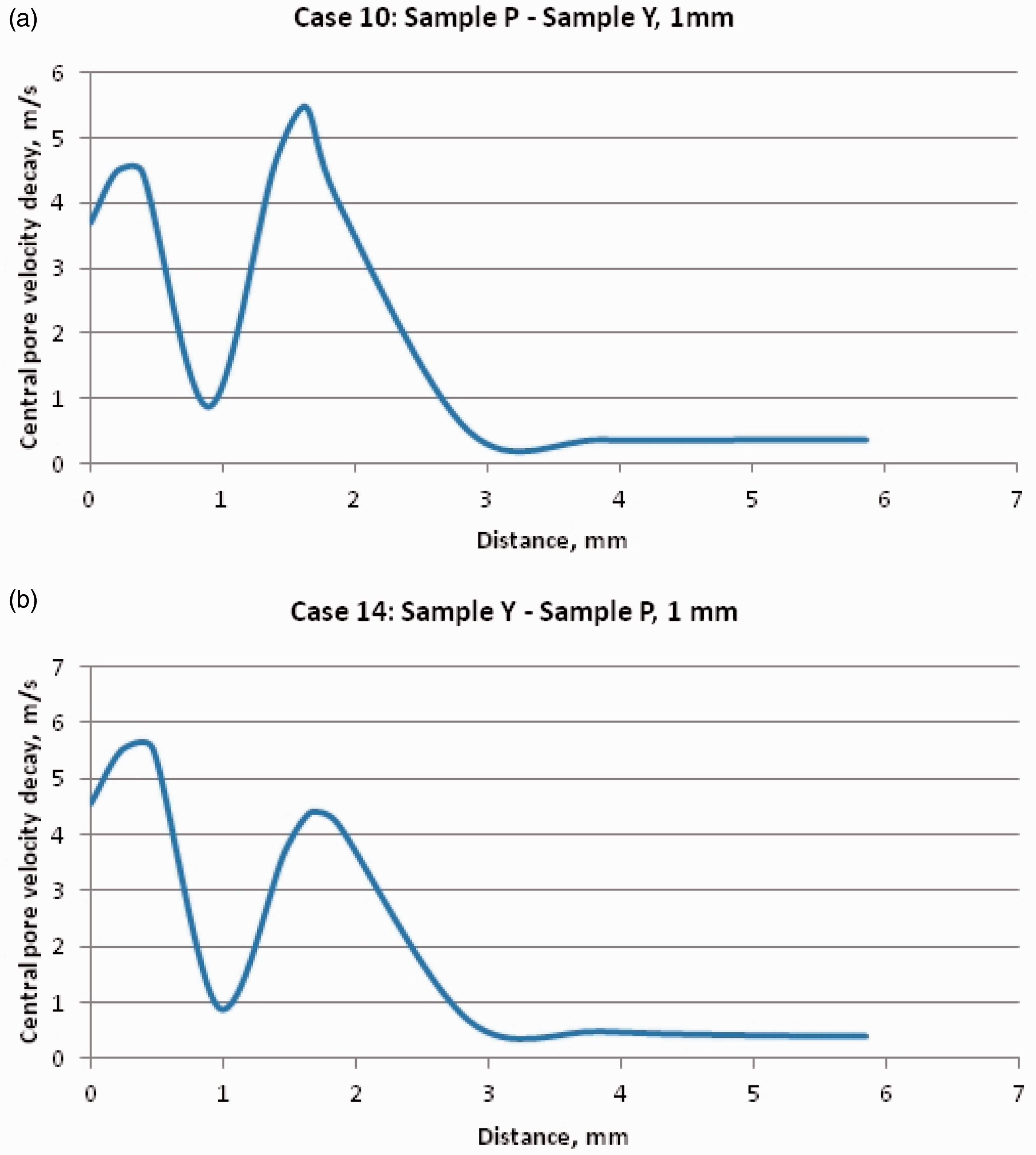

The AP of the ensembles of two layers is calculated having the numerical results for the flow rate of the developed flow Q, m³/s, as follows:

AP = \frac{Q}{A}, m / s

(5)

where A is the area of the textile layer A (area of the domain), m².

The flow is considered to be developed being steady-state, that is, the velocity profile does not change downstream.

The difference between the AP of the cases is not great, as the AP of Case 10 is 0.375 m/s, while that of Case 14 is 0.384 m/s. So the AP of the ensemble is higher when a fabric with lower porosity is placed as a first layer (Case 14).

Sample P and Sample Y have quite similar porosity and average pore area. Therefore, it is interesting to assess the effect of the order of arrangement in the ensembles between Sample K and Sample P. These macrostructures have quite different characteristics (Table 1): Sample K is very porous (51.6%), compared to Sample P, which is more tightly woven and has lower porosity (29.1%). The results for the central pore velocity decay are presented in Figure 7.

Figure 7.

Central pore velocity decay, distance between the layers 0.5 mm: (a) pair Sample K-Sample P (Case 1); (b) pair Sample P-Sample K (Case 5).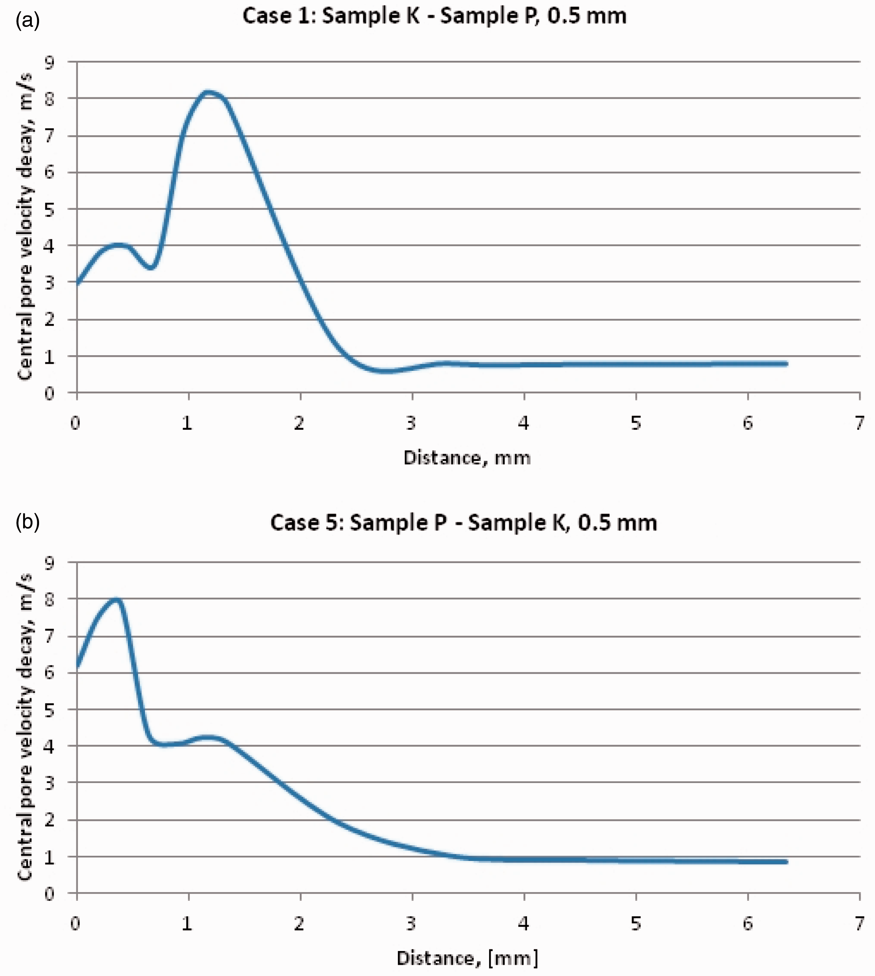

The results prove again the influence of the order of the two samples in the ensemble on the flow development. The flow velocity through Sample K is 4.0 m/s when it is the first layer in the pair (Case 1, Figure 7(a)), and 4.24 m/s, when it is the second layer downstream (Case 5, Figure 7(b)). This means that the flow velocity through Sample K in Case 1 reaches 94% of the maximum velocity through the same sample in Case 5. For comparison, the flow velocity through the more porous layer in Figure 6(a) (Sample P) reaches 98% from the maximum velocity, obtained when Sample P is the second layer in the ensemble.

As for the maximum velocity through Sample P, it is 8.17 m/s when Sample P is the second layer in the ensemble (Figure 7(a)) and 7.9 m/s, when it is the first layer in the ensemble (Figure 7(b)). This means that the maximum flow velocity in Case 5 reaches 97% of the maximum flow velocity in Case 1.

The AP of the textile ensemble in Case 1 is 0.79 m/s, while in Case 5 the AP is 0.85 m/s. This proves the results for Cases 10 and 14 that higher AP of the system of two ensembles is obtained when the fabric with lower porosity is placed as a first layer in the ensemble (Case 5).

The effect of the distance between the layers in the ensembles

Figure 8 shows the numerical results for the velocity magnitude of the flow, passing through the ensembles of Sample K-Sample P, for different distance between the two layers: 0.5 – 1 – 3 – 5 mm (Cases 1–4). Figure 9 represents the velocity magnitude of the same textile macrostructures, but simulated in reverse order: Sample P-Sample K (Cases 5–8).

Figure 8.

Velocity magnitude (m/s) visualization for the ensemble Sample K-Sample P (Cases 1–4) placed at a distance of: (a) 0.5 mm; (b) 1 mm; (c) 3 mm; (d) 5 mm.

Figure 9.

Velocity magnitude (m/s) visualization for the ensemble Sample P-Sample K (Cases 5–8) placed at a distance of: (a) 0.5 mm; (b) 1 mm; (c) 3 mm; (d) 5 mm.

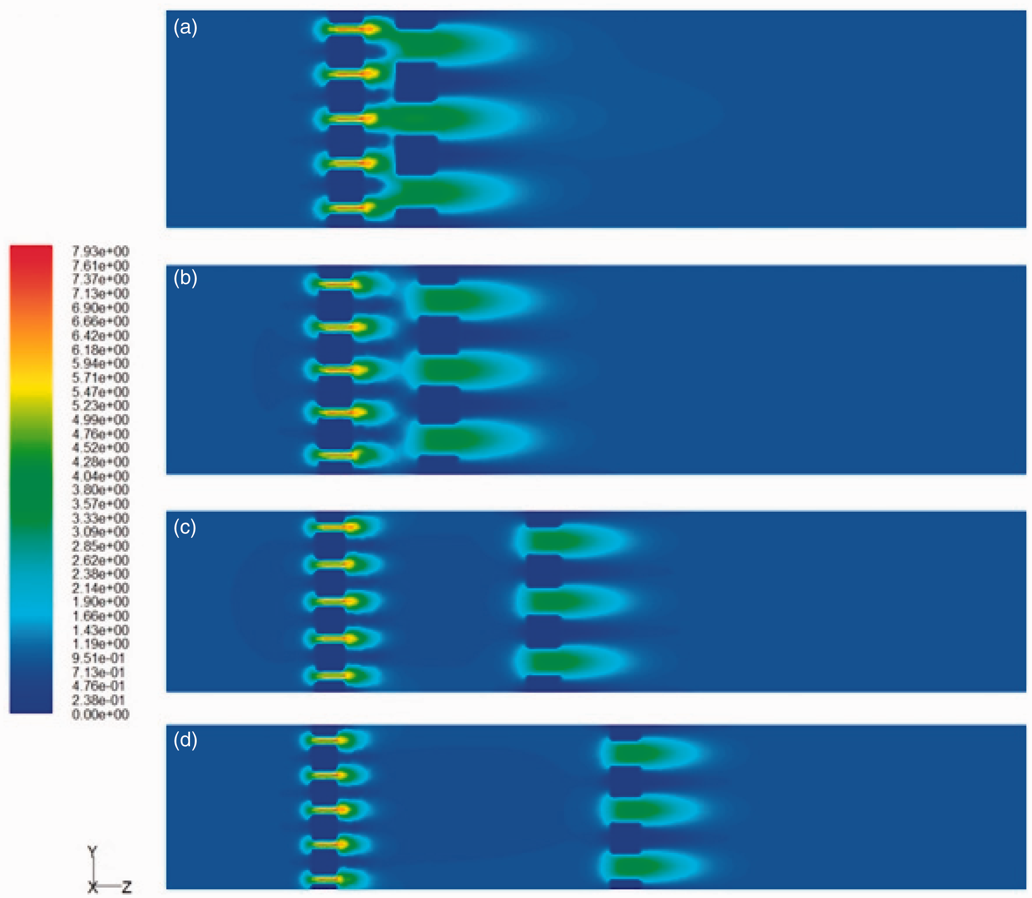
The velocity fields visualize the effect of the distance between the two textile layers, which is, in fact, the thickness of the air gap between the studied woven macrostructures. The air gap plays the role of a “chamber” between the textile layers, visualized very well in Figure 10, where the numerical results for the static pressure are presented.

Figure 10.

Contorurs of the static pressure for the ensamble Sample P-Sample K, Pa: (a) Case 5 (distance 0.5 mm); (b) Case 8 (distance 5 mm).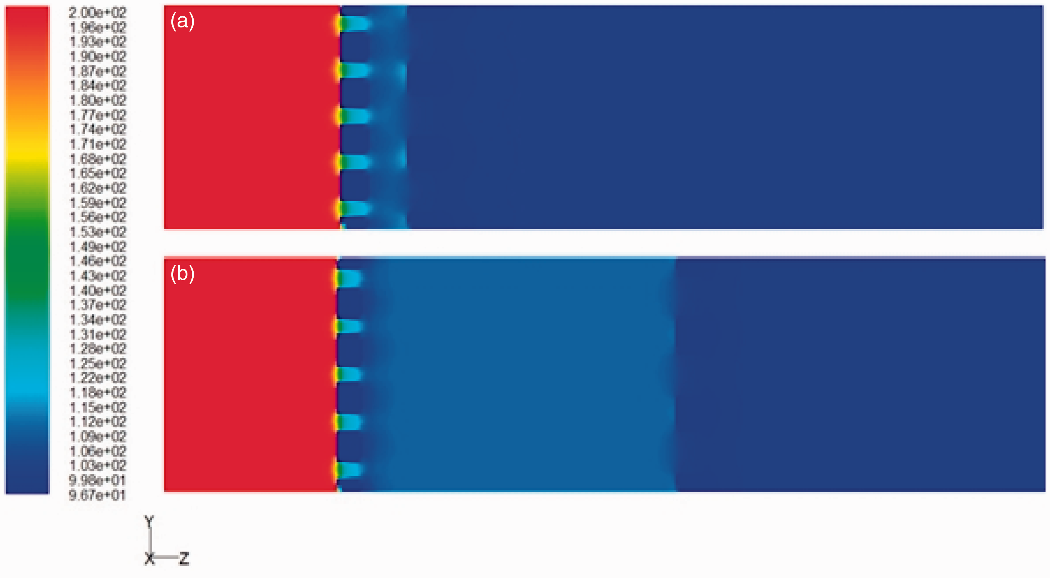

A comparison is made between Case 5, with a distance between Sample P and Sample K of 0.5 mm, and Case 8, where the distance between the same woven structures in the ensemble is 5 mm. The results show that the static pressure changes logically: it is higher before the first layer, decreases in the “chamber” between the two layers and drops down after the second layer, with the flow development downstream.

To assess in detail the influence of the air gap, the velocity decay of the flow through the central pore is presented in Figure 11 for the ensembles Sample K-Sample P (Cases 1–4) and Figure 12, for the ensembles Sample P-Sample K (Cases 5–8).

Figure 11.

Central pore velocity decay for the ensemble Sample K-Sample P (Cases 1–4) for different distances between the layers.

Figure 12.

Central pore velocity decay for the ensemble Sample P-Sample K (Cases 5–8) for different distances between the layers.

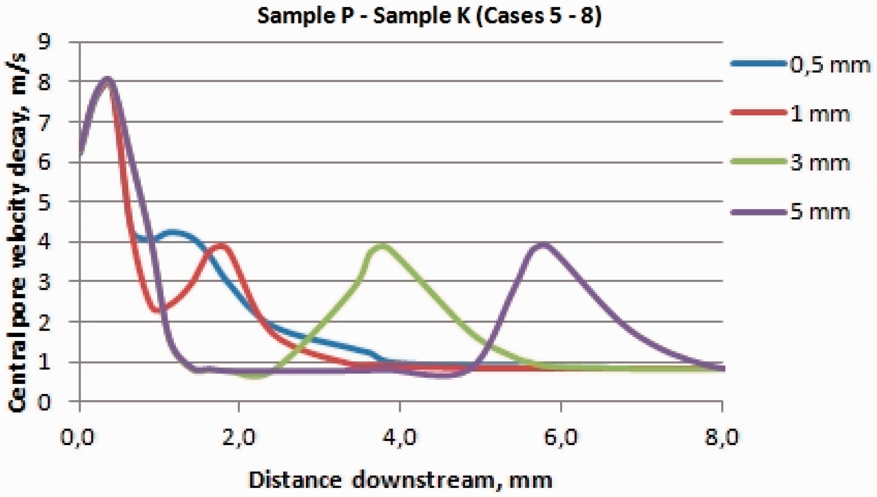
It is obvious that the pick of the maximum velocity magnitude through the second layer of the ensemble moves downstream with the increment of the distance between the two textile macrostructures. Therefore, the flow pattern is completely different within the distance 0–2 mm downstream for Cases 1–4 (Figure 10) and also for Cases 5–8 (Figure 11).

Additional processing of the numerical results is performed in order to better understand the effect of the distance and the order of the layers in the ensemble – the extrema of the flow velocities are visualized, as follows:

Max 1 is the maximal value of the air velocity when passing through the first sample;

Min 1 is the minimum velocity of the flow in the air gap between the samples;

Max 2 is the maximum velocity of the air passing through the second sample;

Min 2 is the minimal air velocity reached after the second sample.

Figure 13 presents the extrema for the ensembles, involving Sample K and Sample P (Cases 1–8). The numerical data show that the largest is the influence of the distance between the layers in the ensemble on the Min 1 and Max 2 velocities, while Max 1 and Min 2 values remain almost constant. The reason is that the air layer between the two textile layers forms a “chamber”, where the flow development is strongly influenced by the length of the air “chamber” and the change in the static pressure. On the other hand, the flow development within the air layer has an effect on the maximum of the air velocity through the second textile layer.

Figure 13.

Maximum and minimum velocity values for Cases 1–8.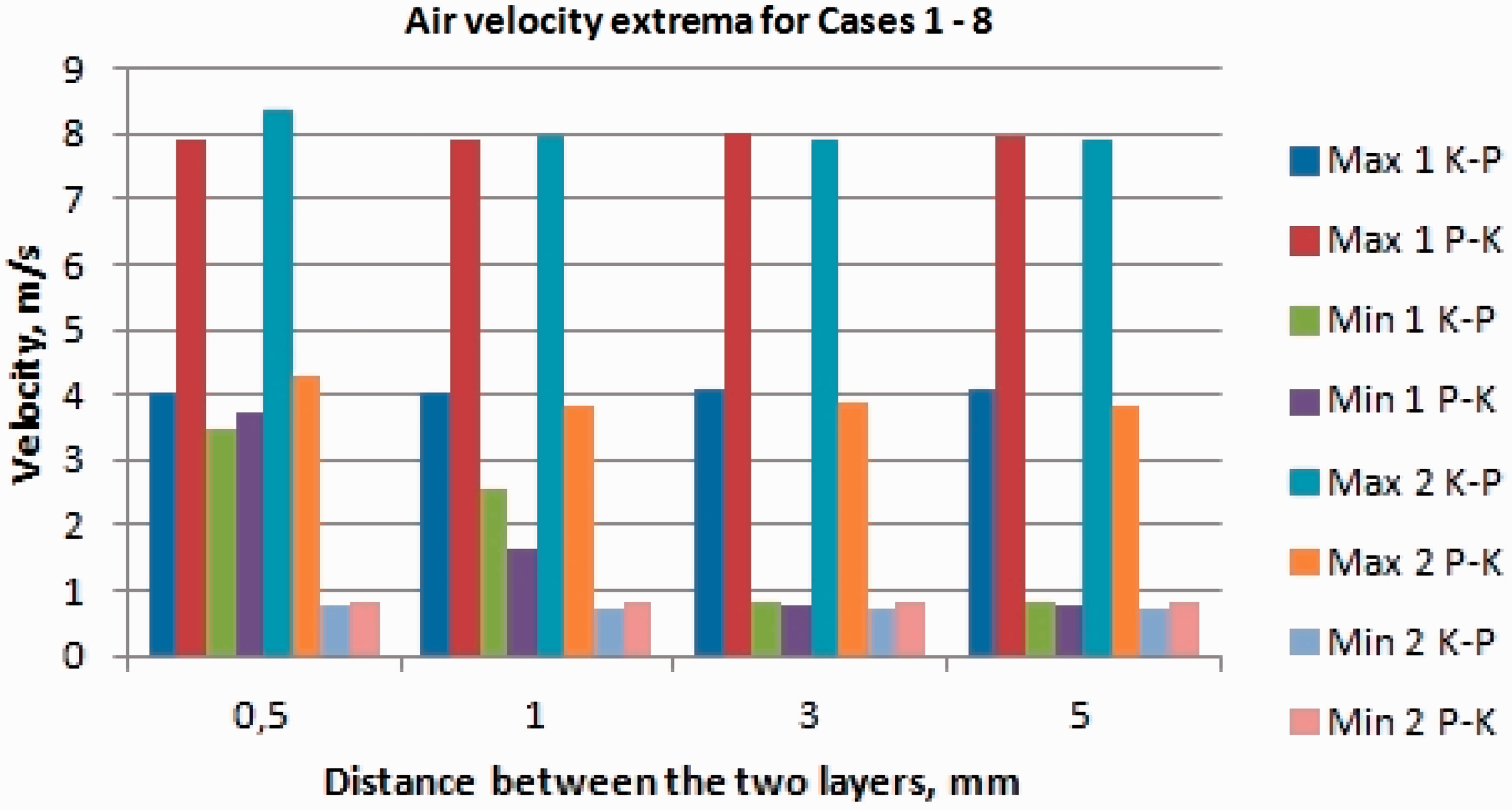

It has to be mentioned also that there is no great difference (if any) between the extrema in the flow velocities when the distance between the two textile layers in the ensemble changes from 3 to 5 mm.

The same analysis of the extrema in the flow velocities for Cases 9–16, shown in Figure 14, leads to similar conclusions: the distance between the two layers affects mainly the Min 1 velocity. In this case, the greater similarity between the characteristics of Sample P and Sample Y leads to almost the same flow development and equal values for flow velocities for the studied distances of 1, 3 and 5 mm between the two samples, despite their order of arrangement in the ensemble. The only difference is between the results for the 0.5 mm distance, compared with 1 mm distance: Max 1, Max 2 and Min 2 values are a little higher for the shortest distance between the textile layers in the ensemble.

Figure 14.

Maximum and minimum velocity values for Cases 9–16.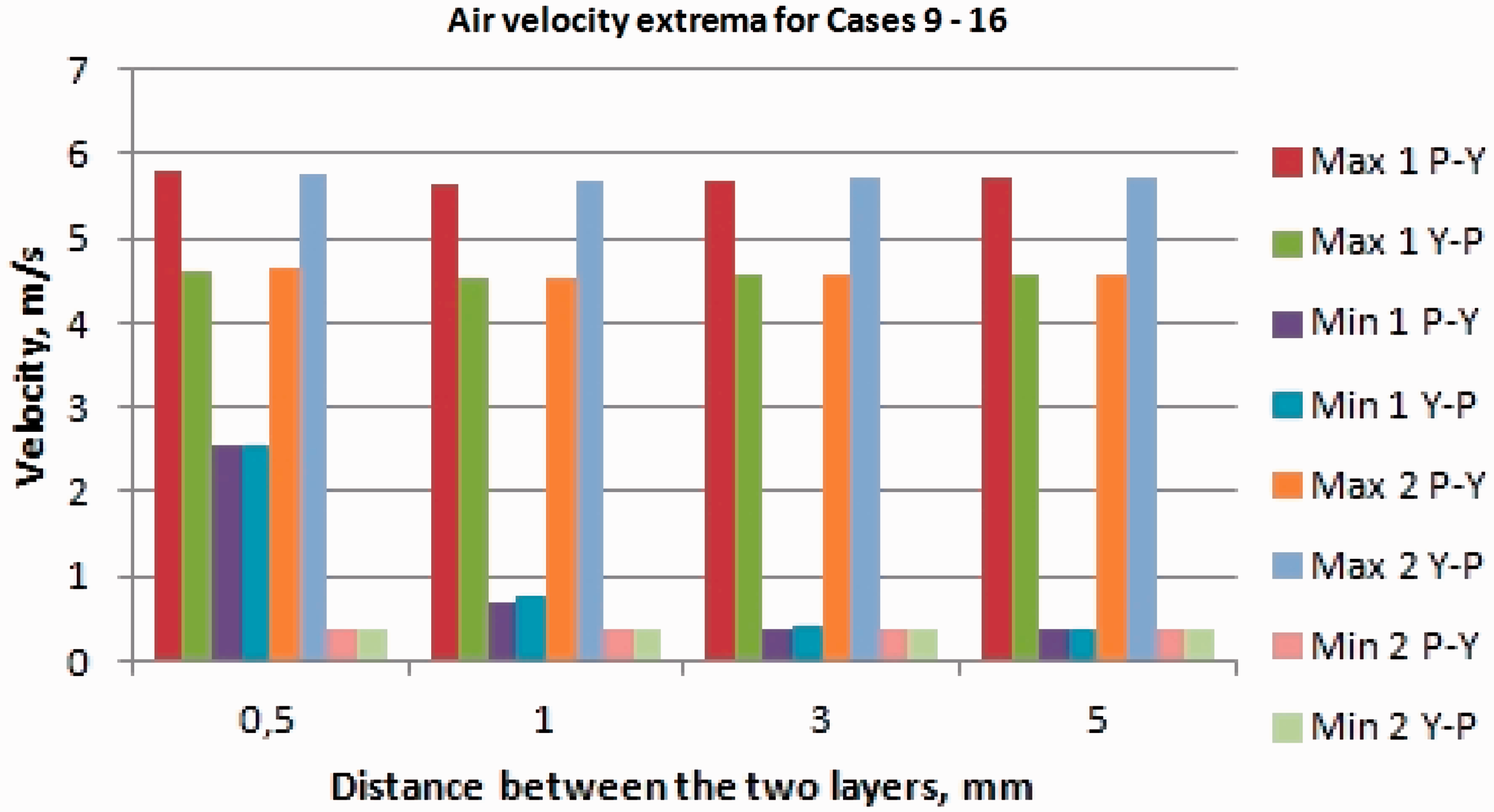

However, in order to ensure better insulation, the velocity of the air flow within the air gap between the two layers has to be as low as possible. Therefore, it can be concluded that the greatest distance between the two textiles, namely 3 and 5 mm, would give better insulation of the ensemble.

The analysis of the AP of each ensemble, calculated on the basis of the flow rate of the developed flow after the second layer, shows that it slightly decreases with the increase of the distance between the textile layers. The largest difference is obtained for the pair Sample K-Sample P, for distances of 0.5, 1 and 3 mm. The effect of the order of the textile layer downstream is also higher for the pair Sample K-Sample P, due to the greater difference in the characteristics of the two layers: despite the difference between the two samples, the ensemble Sample K-Sample P has lower AP than the ensemble Sample P-Sample K.

Conclusions

In this study the AP of ensembles of two woven structures was investigated by means of CFD, using the theory of jet systems. This method was verified and applied successfully for prediction and investigation of the AP of single-layer woven structures. The present study showed the applicability of the approach for modeling the AP of two layers of woven structures.

The analysis of the numerical results for 16 ensembles showed that the AP of the ensembles is strongly influenced by the order of arrangement of the layers and the distance between them.

It was found that higher AP was obtained when a macrostructure with lower porosity was placed as a first layer in the ensemble. It was also found that the distance between the layers had an effect mainly on the flow velocity through the air gap between the two textile layers, as well as on the maximal velocity of the flow through the second layer in the ensemble. The lowest AP was obtained for a distance of 3–5 mm between the layers.

The presented approach can be successfully applied for further studies on the topic of woven structure permeability. The method can be useful also for detailed analysis of a flow after a set of textile barriers.

Footnotes

Declaration of conflicting interests

The authors declared no potential conflicts of interest with respect to the research, authorship and/or publication of this article.

Funding

The authors received no financial support for the research, authorship and/or publication of this article.

References

Angelova

. Textiles and human thermophysiological comfort in the indoor environment, New York: CRC Press, 2016.

Saville

. Physical testing of textiles, Cambridge: The Textile Institute. Woodhead Publishing Ltd, 2003.

Kulichenko

Langenhove

. The resistance to flow transmission of porous materials. J Textil Inst 1992; 83: 127–132.

Wang

. Prediction of the permeability of woven fabrics. J Ind Textil 2005; 34: 243–254.

Belkacemi

Broadbent

. Air flow through textile at high differential pressure. Textil Res J 1999; 69: 52–58.

Jakšić

Porosity of the flat textiles. In: Dubrovski

(ed). Woven fabric engineering, Rijeka, Croatia: InTech, 2010, pp. 255–272.

Ogulata

Mavruz

. Investigation of porosity and air permeability values of plain knitted fabrics. Fibers Textil East Eur 2010; 82: 71–75.

Gibson

Desabrias

Godfreay

. Dynamic permeability of porous elastic fabrics. J Eng Fibers Fabrics 2012; 7: 29–36.

Epps

. Prediction of single-layer fabric air permeability by statistics modeling. J Test Ecal 1996; 24: 26–31.

10.

Nazarboland

Chen

Hearle

. Effect of different particle shapes on the modeling of woven fabric filtration. J Inform Comput Sci 2007; 2: 111–118.

11.

Grouve WJB, Akkerman R, Loendersoor R. et al. Transverse permeability of woven fabrics. In: 11th ESAFORM conference on material forming, Lyon, France, 23–25 April 2008.

12.

Rief

Glatt

Laourine

. Modeling and CFD-simulation of woven textiles to determine permeability and retention properties. AUTEX Res J 2011; 11: 78–83.

13.

Elnashar

. Volume porosity and permeability in double-layer woven fabrics. AUTEX Res J 2005; 5: 207–217.

14.

Padaki

Alagirusamy

Deopura

. multilayer interlocked woven fabrics: simulation of RTM mold filling operation with preform permeability properties. RJTA 2010; 14: 23–34.

15.

Angelova

Stankov

Simova

. Three dimensional simulation of air permeability of single layer woven structures. Cent Eur J Eng 2011; 1: 430–435.

16.

Angelova

Stankov

Simova

. computational modeling and experimental validation of the air permeability of woven structures on the basis of simulation of jet systems. Textil Res J 2013; 83: 1887–1895.

17.

Stankov P. Three dimensional turbulent flows in the heat and mass transfer processes. DSc Thesis, Technical University of Sofia. Bulgaria, 1998.

18.

Mezarsiöz

Ogulata

. Prediction of the air permeability of knitted fabrics by means of computational fluid dynamics. Tekstil ve Konfeksion 2014; 24: 202–211.

19.

Peksen

Acar

Malalasekera

. Computational modelling and experimental validation of the thermal fusion bonding process in porous fibrous media. Proc IMechE Part E J Process Mech Eng 2011; 225: 173–182.