New method for determining the bending modulus of solid and hollow fibers from deflection tests

Abstract

The bending moduli of solid and hollow glass fibers were determined by means of fiber deflection tests. The test method was modified by measuring both the vertical and horizontal displacements of the end of the deflected fiber, without increasing the number of tested fibers, in order to reduce the high scatter of conventional test results obtained by measuring only the vertical displacement. Upper and lower boundary curves of the fiber end displacements were determined to filter out inaccurate measurements, for example, when the neutral line of the fiber is not a plane but a spatial curve. The mean and coefficient of variation of the fiber bending modulus were estimated from the recorded coordinates of the fiber ends, applying two newly-developed statistical evaluation methods based on the individual coordinates or on their average. After comparing several evaluation methods, it was demonstrated that the individual coordinate-based method provided the least relative error of the average.

Keywords

glass fiber deflection test hollow fiber bending modulus

Increasing emphasis has recently been put on energy saving—for example, while traveling, transporting goods, or simply moving objects to save resources and reduce emissions.¹ Polymer matrix composite materials are suitable for energy efficient structures due to their high stiffness and strength combined with low density, and their spread has been steady in the recent decades.² Thermoset polymer composites typically consist of two constituents: fibers (e.g. glass, carbon, aramid) and matrix (e.g. epoxy, unsaturated polyester, and other resins, including bio-based ones).³ The performance of composites can be improved either with advanced matrix materials including hybrid resins,⁴ or with novel fiber types. Most of the mechanical properties of well-designed composites are dominated by the fiber properties, which therefore need to be determined accurately. Novel carbon nanotube-based fiber materials,⁵ fiber forming techniques such as electrospinning,^6–8 and special cross sections, including hollow fibers, are in focus for researchers to improve composite performance and to add various extra functions to the materials.

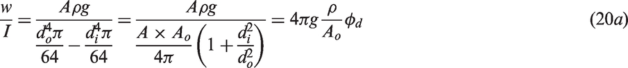
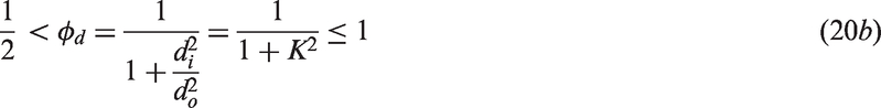
Hucker et al.⁹ used hollow glass fibers (HGF) to improve the compression strength of composite plates. The hollow fibers have higher bending stiffness than solid ones of the same linear density, which may be exploited, similarly to the high area moment of inertia of sandwich structures. Hucker et al. fabricated HGFs with various diameters, and characterized them with the fiber hollow fraction K², defined as the ratio of the inner (d_i) and outer (d_o) diameter of the fibers, as in equation (1)

0 \leq K 2 = (\frac{d_{i}}{d_{o}}) 2 < 1

(1)

Various uni-directional (UD) composite specimens were tested in compression and it was highlighted that the elastic modulus of the composite decreased if the hollow fraction of the fibers was increased. A 10% increase in compressive strength was achieved with K²≈ 0.22. If the elastic modulus of the fibers had been measured—for example, by fiber deflection tests—the compressive response of the plates could have been estimated and analyzed. Boniface et al.¹⁰ reported that composite plates made of hollow fibers had beneficial energy absorption properties. Hucker et al.¹¹ fabricated their hollow fibers from glass tubes. The pre-form was heated up and stretched to low diameter hollow fibers, which were tensile tested. Low fiber wall thickness and high stretching improved the modulus and strength of the fibers.

Rosen et al.¹² investigated solid and hollow glass fibers and their composites, and highlighted that the hollow glass fiber reinforced plastics (HGFRP) have better stiffness and compressive strength than those reinforced by solid fibers.

Bayat and Aghdam¹³ highlighted through finite element (FE) analysis that hollow fibers had better cooling conditions during manufacture than solid ones, and therefore the detrimental residual stress in the fiber due to fast cooling was reduced. Another FE study indicated that the energy absorbing capacity of the composites can be increased with increased fiber hollow fractions. Besides their beneficial mechanical properties, hollow fibers can store healing or damage-indicating fluids,¹⁴ as an alternative to microcapsules.¹⁵

The mechanical properties of fibers—for example, for composite reinforcement—play a key role in most applications, so fiber testing is crucial. Ameriacan Society for Testing and Materials (ASTM) standards D1388 and D5732 (discontinued in 2008) propose bending stiffness measurement methods for textile samples by means of cantilever bending (Option A of ASTM D1388 and ASTM D5732) and loop bending (Option B of ASTM D1388). Although these standard test methods apply to textile strips, their principles are applicable to single fibers as well. The flexibility of single fibers can be measured by bending the fiber into a loop, where the smallest radius of curvature is measured before fracture of the fiber. A significant difficulty of this test method is the measurement of the curvature just before fracture,¹⁶ which may be done by post-processing a recorded video of the test. Another method utilizes a cone to measure the curvature of the fiber loop at break. Tows of fibers are tensile tested in the textile industry with a knot to explore their flexibility. This test can be done on individual fibers as well. There is also a fiber test where two linked U-shaped loops are bonded to paper tabs and pulled until fracture. The bending modulus of individual fibers can be determined from their deflection due to their own weight, with a test similar to the cantilever test (Option A of ASTM D1388 and ISO 4604:2011), as shown on Figure 1. A fiber clamped horizontally at one end exhibits a deformed shape due to its own weight, and the vertical displacement (f_B = −y_B) of the other end can be recorded using a scale.^17,18 The test methods based on deflection due to own weight can be divided into two categories: (a) where the vertical displacement of the end of a given length (l₀) fiber is recorded; or (b) where the specimen length corresponding to a given chord angle (β) is recorded. Figure 1 shows the schematic of the fiber deflection test. Method (a) has various evaluation processes, while method (b), which is suitable for testing fabrics, cloths, and films, as well as fibers,^19,20 is usually executed using a Flexometer (ASTM D1388, D5732 and ISO 4604:2011). The horizontal displacement of the fiber end (Δx_B = l₀–x_B) has not been used for evaluation of the deflection tests so far in the literature, although it could improve the accuracy of the results.

Figure 1.

Geometrical schematic of the fiber deflection test (f_B = –y_B and Δx_B, respectively are the vertical and horizontal displacements of the fiber end, B0 is the end-point of the straight fibre before deflection).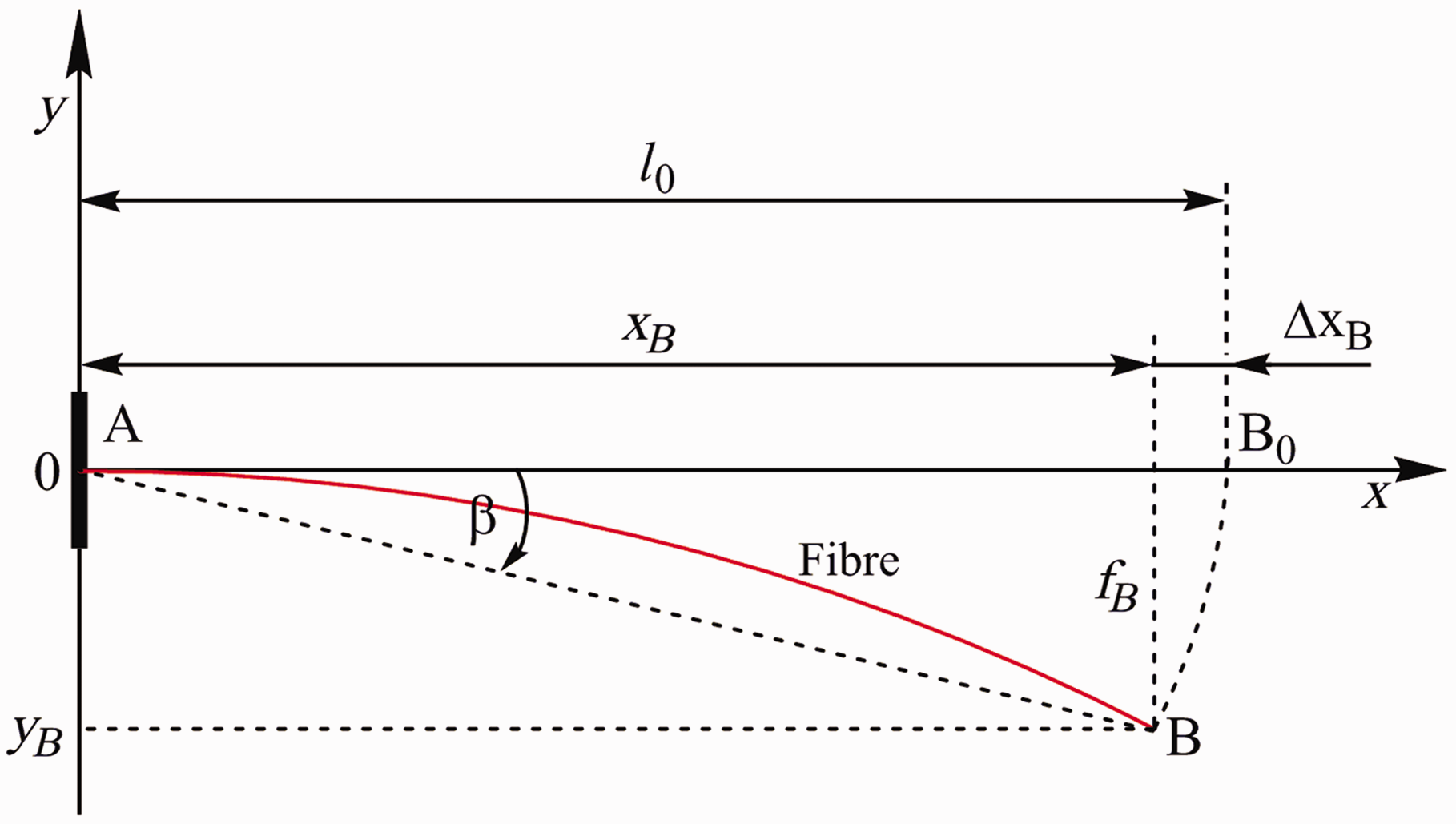

The aim of this paper is to improve the accuracy of the fiber deflection test method by better exploitation of the test data, without increasing the number of samples. The improved evaluation of the test method can result in reduced variability and better bending property estimation of the composites made from the tested fibers.

Materials and methods

The applied hollow fibers were supplied by R&G Faserverbundwerkstoffe GmbH (Germany) in the form of 216 g/m² areal mass woven fabric of twill weave. The solid fibers were manufactured by 3B (Belgium), in the form of continuous tows. The compositions of the two glass fiber types are similar, according to inductively coupled plasma optical emission spectrometry investigations. Fiber types of similar outer diameters were selected for the experiments.

Before the deflection test the geometrical properties, such as outer and inner diameters, were measured on each individual fiber, optically. The measured diameter data (mean and standard deviation) for hollow fibers were d_outer = 13.41 ± 1.32 µm and d_inner = 6.10 ± 1.21 µm (K²= 0.21) while the data for solid fibers was d = 13.77 ± 0.73 µm. Fiber deflection tests were performed earlier on solid and hollow glass fibers of 50 mm length, and evaluated using only the vertical displacements of the fiber ends. Results of these tests have been reported earlier.^18,21,23 The essence of this method is that a fiber is clamped horizontally at one end (Figure 1) and a vertical measuring scale is used to read the vertical displacement (f_B = −y_B) of the free fiber end, with 0.5 mm precision. More accurate results can be obtained if the horizontal displacement (Δx_B) of the fiber end is measured by another scale as well. In order to demonstrate the applicability of this latter evaluation method, further deflection tests were performed on 10 solid and 10 hollow glass fibers.

Results and discussion

Previous results of vertical deflection measurements

Determination of the Young’s modulus through tensile testing of high performance fibers, such as glass, basalt, carbon, or ceramic, may be difficult due to gripping problems (bending fragility, compression fragility of hollow fibers, obliquity, crimp, or slippage from the grips). These may result in defective specimens and various systematic and statistical errors, mainly compromising the accuracy of the elongation values essential for calculating the modulus. Fiber deflection tests were performed on 50 mm long fibers by Kling and Czigany,^18,23 and evaluated using only the vertical displacements of the fibers, according to the calculation method published by Holden.²² The results, including the vertical displacement (y_B) and the bending modulus (E), are shown in Table 1.^18,23

Table 1.

Fiber deflection test results of solid and hollow glass fibers.^18,23 SD, CV, and MRE are the standard deviation, coefficient of variation, and relative error of the mean, respectively

Fiber	Number of tested samples	Fiber end vertical displacement (y_B)				Bending modulus (E)
Fiber	Number of tested samples	Mean (mm)	SD (mm)	CV (%)	MRE (%)	Mean (GPa)	SD (GPa)	CV (%)	MRE (%)
Solid	60	23.21	5.49	24	6	74.48	26.34	35	9
Hollow	100	17.08	6.10	36	7	98.99	55.72	56	11

The deflection tests of hollow fibers provided significantly higher values of mean modulus and coefficient of variation than those of the solid fibers. Some of the possible reasons for deviations and high scatter are inaccuracies of the measurement method, in diameter measurements, or in recording only the vertical displacements of the fibers. Another reason for the high scatter and the deviation in the mean values is the possible eccentricity of the hollow fibers, which can result in the neutral axis of a deflected fiber not forming a plane curve, as is assumed for the evaluation. The out-of-test-plane distance of the end point of such an eccentric fiber can reduce its apparent vertical displacement, and consequently increase the apparent elastic modulus calculated from the measurements. In order to eliminate the above mentioned problems, both the fiber deflection test method and the evaluation process were improved to enable more accurate determination of the fiber modulus, based on the classical bending theory and measured values of both the vertical and horizontal displacements of the fiber end.

Calculation of large fiber deflections

The following conditions were assumed: the fiber is flexible (i.e. has a finite bending stiffness), has a circular cross section, the fiber diameter, d, is constant and small, the elongation of the fiber is negligible compared to its bending deflection, and the effect of shear force is negligible. The material of the fiber is linearly elastic, and the equations of classic bending theory can be applied (e.g. the deflected shape of the fiber is a plane curve and its cross sections remain planar).

The deflection of the fiber due to its own weight increases if the free length of the fiber is increased, but the change in fiber length due to deflection is negligible. Therefore the arc length between two points of the deformed shape, Δs, always equals the original distance, Δx₀, of the same points. According to the above assumptions, s = x₀ during the calculation of bending moment along the fiber. Parameters of the deflected fiber shape and the schematic of the forces acting on the arc element are summarized in Figure 2.

Figure 2.

Schematic of the forces acting on an arc element of the deflected fiber (y_B = y(l₀)).

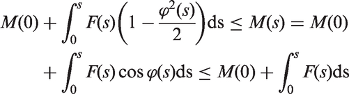
It is most practical to describe the fixed length deflected shape of the fiber along its length as a function of the arc length (distance along the fiber), s, and the angle, ϕ, of the tangent at any point, where x(s) and y(s) are the coordinates of a given point and w (N/mm) is the distributed load that is the specific fiber weight. The moment, M(s), on an arc element can be estimated with lower and upper bounds according to equation (2) based on inequality (3)

M (0) + \int_{0}^{s} F (s) (1 - \frac{ϕ 2 (s)}{2}) ds \leq M (s) = M (0) + \int_{0}^{s} F (s) \cos ϕ (s) ds \leq M (0) + \int_{0}^{s} F (s) ds

(2)

0 < 1 - \frac{ϕ 2 (s)}{2} \leq \cos ϕ (s) \leq 1

(3)

According to the basic assumptions detailed earlier, the classic bending theory is applied as in equation (4)

M = EI \frac{1}{R} = EI κ

(4)

where I is the second moment of inertia of the fiber cross section, which gives the bending stiffness IE, together with the bending modulus, E, of the fiber. R is the radius of curvature, and κ = 1/R = dϕ/ds is the curvature. Equation (4) can be written in an integro-differential equation form, which yields equation (5) after differentiation

\frac{d 2 ϕ}{ds 2} = \frac{F (s)}{EI} \cos ϕ (s) = \frac{w}{EI} (l_{0} - s) \cos ϕ (s)

(5)

The second order non-linear differential equation (5) cannot be solved analytically, therefore upper and lower bounds are determined first using inequality (2), and then numerical methods are applied for a more accurate solution.

Boundary curves of the fiber end positions

The upper bound of $\cos ϕ (s) \leq 1$ , part of inequality (3) is given first in equation (6)

\frac{d 2 ϕ}{ds 2} = \frac{F (s)}{EI} \cos ϕ (s) = \frac{w}{EI} (l_{0} - s) \cos ϕ (s) \leq \frac{w}{EI} (l_{0} - s)

(6)

Therefore the differential inequality can be written as in equation (7)

\frac{d 2 ϕ}{ds 2} \leq \frac{w}{EI} (l_{0} - s)

(7)

Integration of equation (7) yields:

κ (s) = \frac{d ϕ}{ds} \leq C_{1} + \frac{w}{EI} (l_{0} s - \frac{s 2}{2}) = C_{1} + \frac{{wl}_{0}^{2}}{2 EI} (2 \frac{s}{l_{0}} - \frac{s 2}{l_{0}^{2}})

(8)

Integration constant, C₁, can be determined if we consider that the curvature is zero at the free end of the fiber at s = l₀, as given in equation (9)

κ (l_{0}) = C_{1} + \frac{{wl}_{0}^{2}}{2 EI} = 0 \Rightarrow C_{1} = - \frac{{wl}_{0}^{2}}{2 EI}

(9)

Equation (8) gives a negative curvature for the deflected fiber shape if C₁ is substituted according to equation (10), which agrees with Figures 2 and 3

κ (s) = \frac{d ϕ}{ds} = - \frac{{wl}_{0}^{2}}{2 EI} (1 - \frac{s}{l_{0}}) 2

(10)

Figure 3.

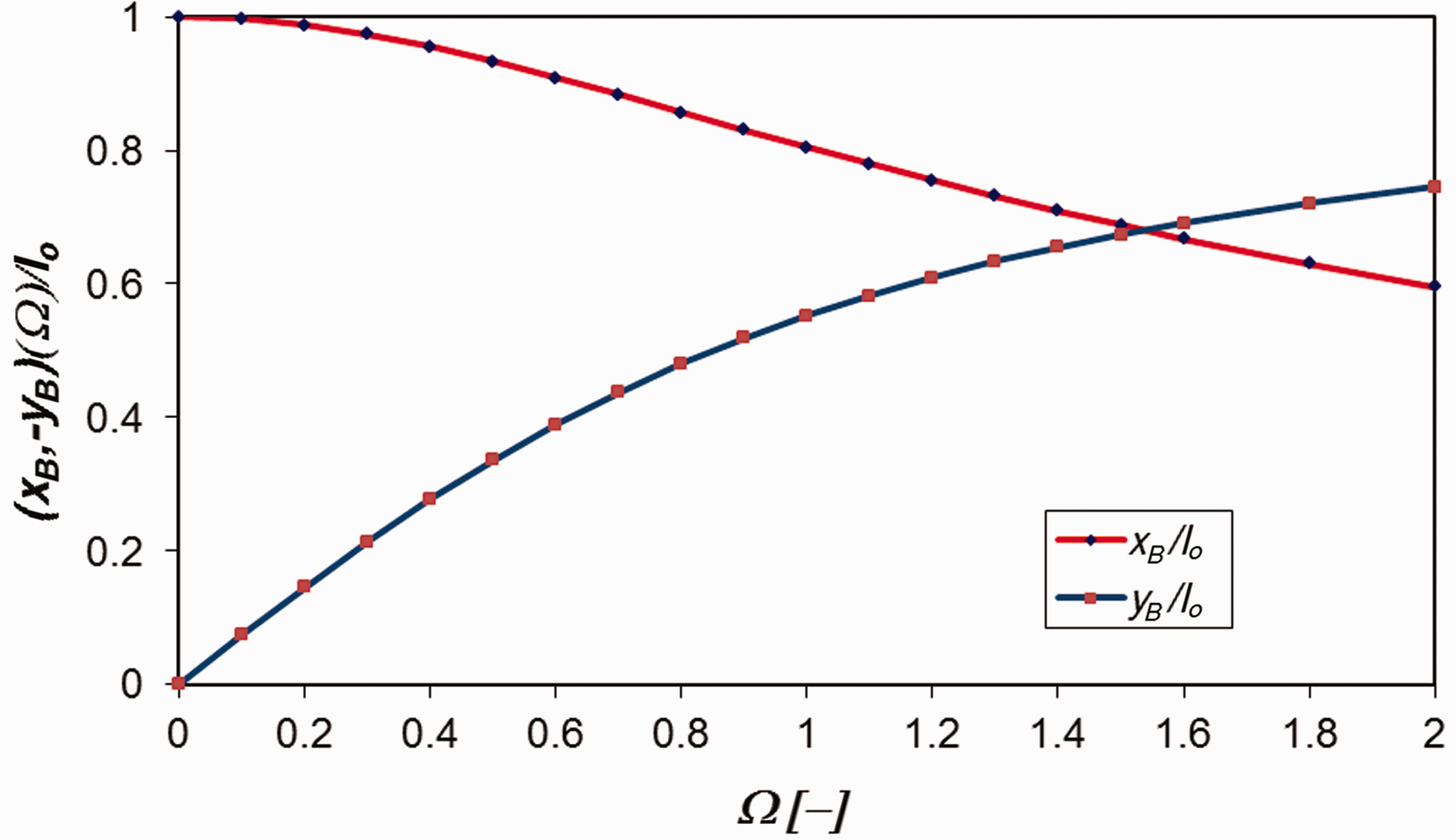
Normalized coordinates of the fiber end as a function of parameter Ω.

Equation (10) indicates that the essence of the upper boundary estimation is that x₀ = s is also considered when calculating the moments. Moments higher than the actual ones are used, therefore, which results in over-estimated absolute curvature values. In the case of cosϕ = 1 the expression of the elementary lever-arm in equation (2) changes from cosϕds into ds, and this simplification results in a kind of uniformly distributed force system, where the forces acting on the arc elements point to the direction of the centre of curvature instead of being vertical.

Equation (10) can be integrated, considering ϕ(0) = 0, to obtain the tangent angle of the estimated fiber shape. The arranged form of equation (11) shows that the angle of the tangent is always negative along the fiber (0 ≤ s ≤ l₀), which agrees with Figure 2

ϕ (s) = - Ω (1 - (1 - \frac{s}{l_{0}}) 3), Ω = \frac{{wl}_{0}^{3}}{6 EI}

(11)

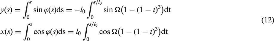
The fiber length dependent Ω constant is one sixth of Holden’s k constant. The parametric equations of the fiber shape with 0 ≤ t = s/l₀ ≤ 1 can be calculated using ϕ(s), as given in equation (12).

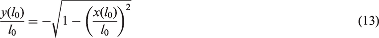
y (s) = \int_{0}^{s} \sin ϕ (s) ds = - l_{0} \int_{0}^{s / l_{0}} \sin Ω (1 - (1 - t) 3) dt x (s) = \int_{0}^{s} \cos ϕ (s) ds = l_{0} \int_{0}^{s / l_{0}} \cos Ω (1 - (1 - t) 3) dt

(12)

The lower boundary curve of the fiber deflection can be generated, if the curvature of the fiber is assumed to be zero all along its length—that is, the fiber remains straight and the fiber is rotated around the fixed end, which is transformed into a hinge. Consequently, the curve of fiber end-point is a circular arc, described by equation (13)

\frac{y (l_{0})}{l_{0}} = - \sqrt{1 - (\frac{x (l_{0})}{l_{0}}) 2}

(13)

where the end-point coordinates are x_B = x(l₀) and y_B = y(l₀), as indicated in Figures 1 and 2.

All the experimental data points of the solid fibers fall between the boundary curves, but four of those of the hollow fibers (including two overlapping ones) falls outside the boundary for maximum curvature, probably due to measuring artifacts (see Figure 4). These are excluded, with the aid of the boundary curves, to increase the accuracy of the remaining data points. A significant scatter is identified in the test data, therefore an accurate solution between the boundary curves is yet to be found for the correct determination of the average elastic modulus of the fibers.

Exact solution using the fourth-order Runge–Kutta method

The so-called fourth-order Runge–Kutta method²⁴ is an effective numerical tool for solving ordinary differential equations. It provides explicit solutions applying recursive formulae for calculating the next value of the ordinate from the weighted sum of four former ones and a finite abscissa increase. It is primarily used for first order differential equations and initial value problems, but it can be applied successfully to solve boundary value problems of higher order equations by using the so-called shooting method, based on iterations.²⁴ As the fourth-order Runge–Kutta method provides fourth-order accuracy (fifth-order error) the same fifth-order error definition was applied in calculations performed with Microsoft Excel. The normalized arc length interval of [0,1] was divided into 100 equal sections, and the calculations were executed with a step size of Δt = 0.01. Figure 3 shows the calculated coordinates of the fiber end-point as a function of parameter, Ω. These curves correspond to those calculated by Holden.²²

New evaluation method and test results

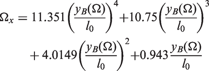
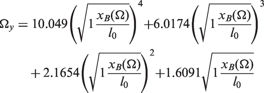
The curves of Figure 3 can be considered as parameterized inverse functions from the test evaluation point of view, since the measured values are the (Δx_B = l₀–x_B, f_B = −y_B) displacement components of the fiber end-point, and Ω is the parameter to be determined. The polynomial trends of the normally-measured y and the previously-not-exploited x normalized coordinates of the fiber end-point were used to determine the Ω parameter explicitly, with high coefficient of determination ( R ²≥ 0.9998). Equations (14) and (15) can directly be used for test evaluation, determining Ω from the measured coordinates of the fiber end (y_B < 0, f_B = −y_B in Figures 1 and 2)

Ω_{x} = 11.351 (\frac{y_{B} (Ω)}{l_{0}}) 4 + 10.75 (\frac{y_{B} (Ω)}{l_{0}}) 3 + 4.0149 (\frac{y_{B} (Ω)}{l_{0}}) 2 + 0.943 \frac{y_{B} (Ω)}{l_{0}}

(14)

Ω_{y} = 10.049 (\sqrt{1 \frac{x_{B} (Ω)}{l_{0}}}) 4 + 6.0174 (\sqrt{1 \frac{x_{B} (Ω)}{l_{0}}}) 3 + 2.1654 (\sqrt{1 \frac{x_{B} (Ω)}{l_{0}}}) 2 + 1.6091 \sqrt{1 \frac{x_{B} (Ω)}{l_{0}}}

(15)

In the case of a Flexometer, the l₀ fiber length belonging to a given β angle of the fiber chord (Figure 1) is measured, and the parameter, Ω, containing l₀, according to equation (11), can be estimated with a second order polynomial as a function of tanβ = −y_B/x_B with a good agreement (R²≈ 1), as follows.

Ω_{y / x} = 0.2446 (\tan β) 2 + 1.2919 \tan β

(16)

Figure 4 shows the measured coordinates of the fiber end-point and the boundary curves according to equations (12) and (13), as well as the fiber-end curve, determined with the fourth-order Runge–Kutta method, which runs in the middle of the area between the boundary curves.

Figure 4.

Measured coordinates of fiber end-points, boundary curves, and the fiber-end curve determined with the Runge–Kutta method.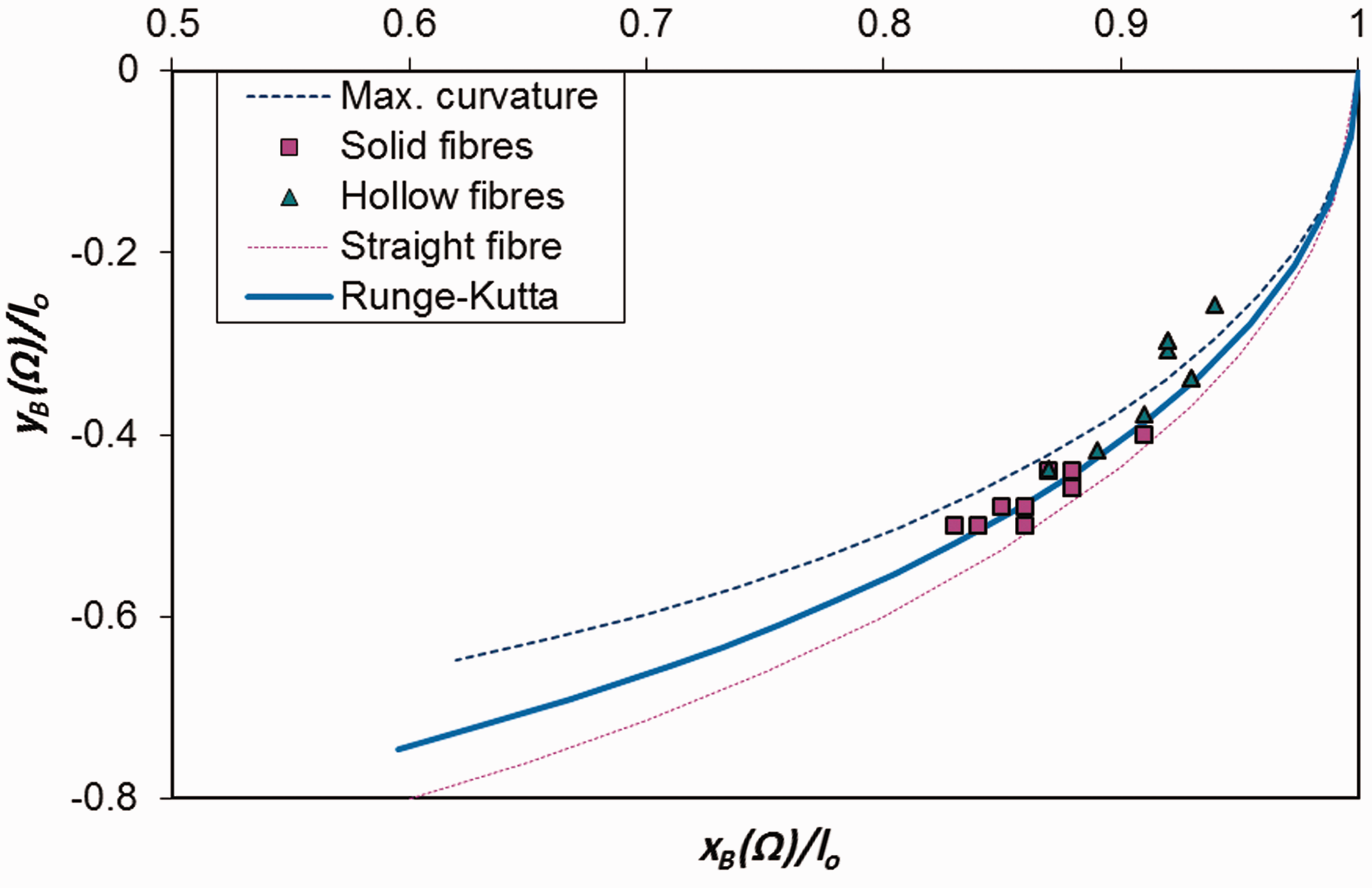

The end-point curve generated by using the Runge–Kutta method, can be described with a simple second order polynomial with excellent fit (R²= 0.9999), where the independent variable is a square root type expression given by

\frac{- y_{B} (Ω)}{l_{0}} = - 0.3369 (\sqrt{1 - \frac{x_{B} (Ω)}{l_{0}}}) 2 + 1.3939 \sqrt{1 - \frac{x_{B} (Ω)}{l_{0}}}

(17)

Figure 5 shows this simple description graphically, where the measured positions of the fiber end-points are also marked.

Figure 5.

Fiber end-point curve after transforming the independent variable.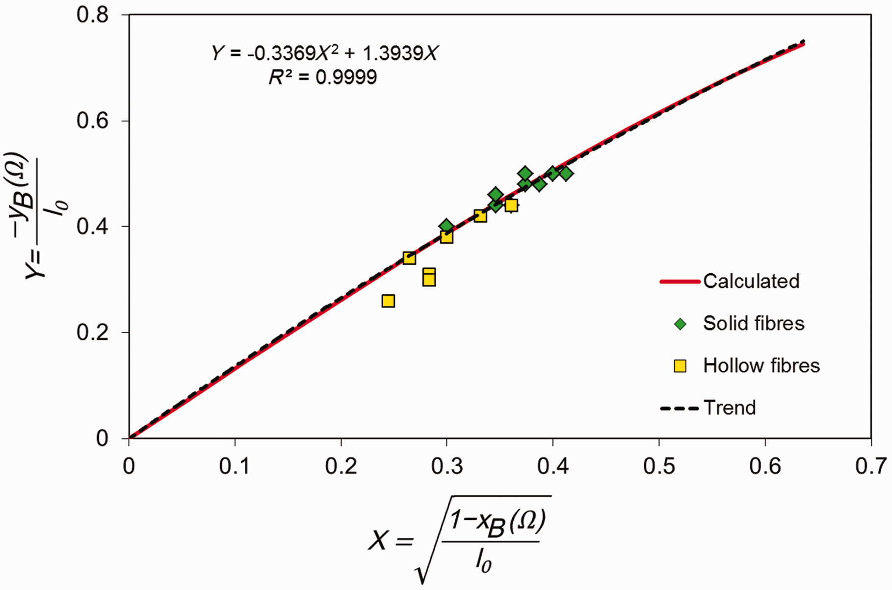

As is usual in the literature, by measuring a single value, such as coordinate y or x, or angle β, the parameter Ω can be calculated with equations (14), (15), or (16), respectively, while measuring, for example, the end-point coordinates y_B and x_B simultaneously provides two estimations for Ω by using equations (14) and (15). These latter two differ because of errors in the measurements (in the fiber length, end-point position, fiber diameter, and roundness) and possible material inhomogeneities (e.g. in elastic modulus or density). Hence, due to measuring errors and inhomogeneities, the measured points scatter around the theoretical end-point curve (points marked with ‘*’ in Figure 6) or, moreover, they may gather around deviated curves above or below the right curve (points marked by “x” or “o” in Figure 6). The possible positions of the measured end-point sets are depicted in Figure 6. This is also true for the average points of these possible end-point sets (marked by red and blue “O” in Figure 6) that are determined by the mean values of the measured end-point coordinates. (For the sake of simpler illustration, in Figure 6 the intersection points of the coordinate lines of the red and blue average points are equal to those created by these coordinate lines and the theoretical end-point curve)

Figure 6.

Three possible positions of the measured end-point sets (x, *, o) and their average points (red, cyan, and blue O) and intersection points (black O) of the theoretical end-point curve and the coordinate lines of average points red and blue.

The estimated values of the Ω parameter from both coordinates are consistent with each other only if the measured points scatter along the correct curve. If the end-points evaluated from x and y coordinates aggregate around separate points away from the correct curve, they yield different Ω for x and y coordinates. Therefore, it is worth considering an averaging-based evaluation method, which exploits both coordinates of each fiber end-point (unlike conventional approaches using only one coordinate). Two suitable methods can be proposed: the method of average points and the method of individual coordinates.

Average point method

If the average point determined by the measured coordinates x and y does not fall onto the correct curve, the best estimation can be obtained by normal projection of the experimental average point onto the correct curve, calculated by the Runge–Kutta method. Such a point can be obtained as follows. Intersecting the correct curve with the coordinate lines running through the average point separately gives two intersection points on the correct curve, as shown on Figure 6 (black “O”s). The midpoint of the chord between the intersection points, which can be obtained as an average, provides a good estimation for the right projected point on the correct curve (cyan “O”). The corresponding parameter Ω can be determined by calculating the Ω values directly from the intersection points separately for the coordinates y and x (Ω_y and Ω_x) using equations (14) and (15), and their average is then computed with equation (18)

\bar{Ω} : = \frac{1}{2} ({\bar{Ω}}_{x} + {\bar{Ω}}_{y}) = \frac{1}{2 n} (\sum_{i = 1}^{n} Ω_{x, i} + \sum_{i = 1}^{n} Ω_{y, i})

(18)

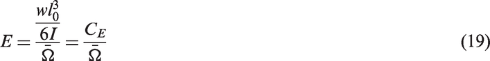
The tensile elastic modulus (E) of the fiber can be obtained from equation (19)

E = \frac{\frac{{wl}_{0}^{3}}{6 I}}{\bar{Ω}} = \frac{C_{E}}{\bar{Ω}}

(19)

where the constant, C_E, is defined by equation (19) and determined by the fiber geometry and material. For a hollow fiber with outer and inner diameters d_o and d_i, and the cross-sectional areas calculated with them, A_o =

d_{o}^{2}

π/4 and A_i =

d_{i}^{2}

π/4, respectively, the terms including cross-sectional geometric parameters can be formulated as in equation (20)

\frac{1}{2} < φ_{d} = \frac{1}{1 + \frac{d_{i}^{2}}{d_{o}^{2}}} = \frac{1}{1 + K 2} \leq 1

(20b)

where A = A_o − A_i is the cross-sectional area of the hollow fiber, while d_i = 0 and

φ_{d}

= 1 are true for solid fibers.

The average point method can be applied effectively to determine the average modulus of the fibers if the fiber geometry is consistent or its parameters are of small standard deviations, so that C_E can be assumed constant. Otherwise, assessing the error of the modulus is problematic due to non-linearity in the formulations.

Individual coordinates method

In this case the coordinates of each measured end-point (P_i) are handled separately. Ω _x,i and Ω _y, _I , determined for the x_i and y_i coordinates of each P_i, are not averaged, but the individual E_x,i and E_y,I values are calculated with the corresponding C_Ei and averaged according to equation (21)

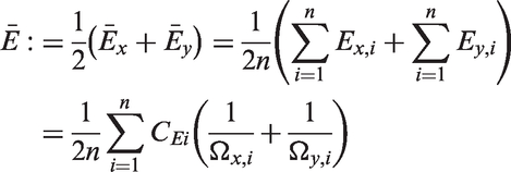
\bar{E} : = \frac{1}{2} ({\bar{E}}_{x} + {\bar{E}}_{y}) = \frac{1}{2 n} (\sum_{i = 1}^{n} E_{x, i} + \sum_{i = 1}^{n} E_{y, i}) = \frac{1}{2 n} \sum_{i = 1}^{n} C_{Ei} (\frac{1}{Ω_{x, i}} + \frac{1}{Ω_{y, i}})

(21)

Alternatively to the average point method, the reciprocals of the Ω parameters calculated from the individual coordinates of the end-points are averaged here. The error of $\bar{E}$ average values can be estimated with the experimental standard deviation, S_E, of the individual values. It is assumed that the error of the individually measured x and y end-point coordinates are independent, thus the 95% confidence intervals and the δ _E relative errors can be written as in equation (22)

E \approx \bar{E} \pm t_{n, 95 %} \frac{S_{E}}{\sqrt{n}} = \bar{E} (1 \pm t_{n, 95 %} \frac{S_{E} / \bar{E}}{\sqrt{n}}) = \bar{E} (1 \pm δ_{E})

(22)

where S_E is the standard deviation of the individual E values and t_n,95% is the relevant critical value of the Student distribution.²⁵

Demonstration of applicability

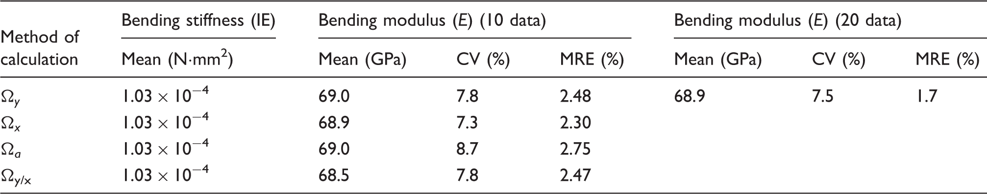
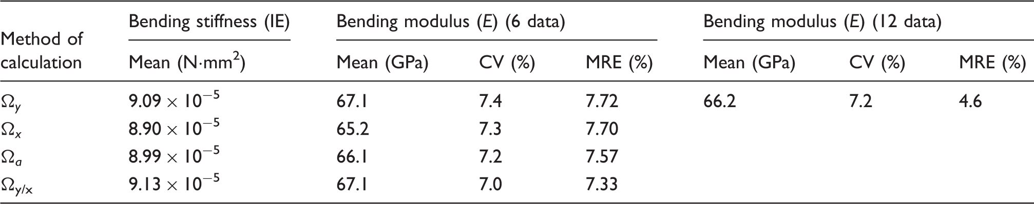
Tables 2 and 3 present the bending modulus values (E) calculated with different approaches from Ω _x , Ω _y , Ω _A and Ω_Y/X based on the results of 10 deflection measurements carried out on solid and hollow glass fibers. The tables contain the average (Mean) bending modulus (E) calculated with equation (21), the coefficient of variation (CV) and the relative error of the mean value (MRE; 10 data: t_n,_95% = 2.262). The Ω _A parameter of a fiber was calculated as the average of the individual values Ω _x and Ω _y using equations (15) and (14), while Ω_y/x was determined using equation (16).

Table 2.

Calculated parameters for solid fibers

Method of calculation	Bending stiffness (IE)	Bending modulus (E) (10 data)			Bending modulus (E) (20 data)
Method of calculation	Mean (N·mm²)	Mean (GPa)	CV (%)	MRE (%)	Mean (GPa)	CV (%)	MRE (%)
Ω _y	1.03 × 10⁻⁴	69.0	7.8	2.48	68.9	7.5	1.7
Ω _x	1.03 × 10⁻⁴	68.9	7.3	2.30	68.9	7.5	1.7
Ω _a	1.03 × 10⁻⁴	69.0	8.7	2.75
Ω_y/x	1.03 × 10⁻⁴	68.5	7.8	2.47

Table 3.

Calculated parameters for hollow fibers before discarding the outlier data points

Method of calculation	Bending stiffness (IE)	Bending modulus (E) (10 data)			Bending modulus (E) (20 data)
Method of calculation	Mean (N·mm²)	Mean (GPa)	CV (%)	MRE (%)	Mean (GPa)	CV (%)	MRE (%)
Ω _y	1.10 × 10⁻⁴	69.5	8.4	2.64	71.6	9.7	2.2
Ω _x	1.17 × 10⁻⁴	73.6	11.1	3.51	71.6	9.7	2.2
Ω _a	1.04 × 10⁻⁴	66.1	6.9	2.18
Ω_y/x	1.17 × 10⁻⁴	73.6	11.0	3.47

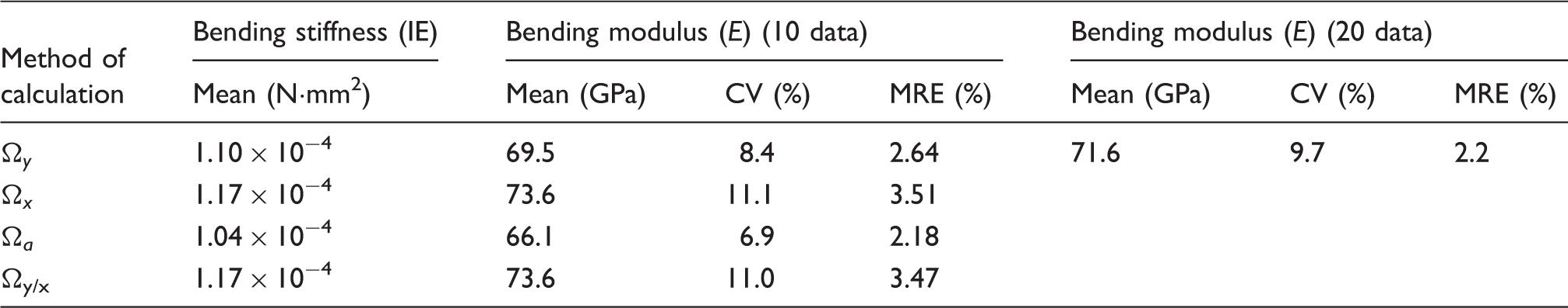
The following observations can be made from analyzing the data in the tables.

The difference between the Ω _x and Ω _y based mean E values (ten data) is minor (<0.15%) for the solid fibers, but in the case of the hollow fibers, the difference is much higher (∼6%).

The CV of the bending modulus for the hollow fibers (8.4–11.1%) is higher than that of the solid fibers (7.3–7.8%).

The individual coordinate method (20 data; t_n,95% = 2.093) is the most advantageous, which gives the lowest relative error of the mean value (MRE) for both the solid (1.7%) and the hollow (2.2%) fibers.

The high scatter is attributed mainly to the four data points lying out of the boundary curves in the case of the hollow fibers. Discarding these four outliers, the remaining points fit very well to the end-point curve (Figure 4). As a consequence, the CV decreased from 9.7% to 7.2% (20 and 12 data), while the MRE (six data: t_n,95% = 2.571; 12 data: t_n,95% = 2.201) increased from 2.2% to 4.6%, as can be seen in Table 4. The increase in MRE, despite of the reduction in CV, follows from the decrease in the number of data (20 → 16) and the mean (71.6 GPa → 66.2 GPa). The latter was due to the effect that the outliers belonged to apparently stiffer fibers with smaller vertical displacement. This error was probably caused by out-of-plane displacements of the fiber end-points (see Figure 4).

Table 4.

Calculated parameters for hollow fibers after discarding the outlier data points

Method of calculation	Bending stiffness (IE)	Bending modulus (E) (6 data)			Bending modulus (E) (12 data)
Method of calculation	Mean (N·mm²)	Mean (GPa)	CV (%)	MRE (%)	Mean (GPa)	CV (%)	MRE (%)
Ω _y	9.09 × 10⁻⁵	67.1	7.4	7.72	66.2	7.2	4.6
Ω _x	8.90 × 10⁻⁵	65.2	7.3	7.70	66.2	7.2	4.6
Ω _a	8.99 × 10⁻⁵	66.1	7.2	7.57
Ω_y/x	9.13 × 10⁻⁵	67.1	7.0	7.33

By measuring both the vertical and the horizontal coordinates of the fiber end-point, and using the individual coordinate method for evaluation, the MRE of the elastic modulus was reduced to 69% or 83% of the original values for the solid and hollow fibers, respectively. In addition, discarding the outliers, by using the determined boundary curves, reduced the number of valuable data points for hollow fibers, but decreased the CV as well. In the case of much more test data, filtering could also be advantageous for the MRE.

Conclusion

The elastic modulus of solid and hollow fibers was determined from fiber deflection tests. Our previous work highlighted that taking only the vertical displacement of the fiber end-point into account results in excessive error and high scatter. In order to reduce the errors, the horizontal displacement was measured as well. The theoretical curve of the fiber end-point was determined with the Runge–Kutta method, and upper and lower boundary curves were found which allowed the identification and filtering of the outliers that were obviously erroneous data points. To make the best use of the test data, two statistical evaluation methods were developed. In order to demonstrate the applicability of the methods developed, some fiber deflection tests were performed on solid and hollow glass fibers. Evaluation using the individual coordinate method resulted in 17–31% reduction in the relative error of the determined mean elastic modulus of the solid and hollow fibers. Discarding four outlier data-points by using the boundary curves provided a 26% reduction in CV for the hollow fibers.

Consequently, the new method can improve the accuracy of modulus evaluation without increasing the number of tested fibers, and it therefore provides more accurate input for analysis of the stiffness of composite structures than the conventional method using only the vertical displacement of the fiber end-point. A future task could be the extensive validation of the new evaluation method on various fiber types.

Footnotes

Declaration of conflicting interests

The authors declared no potential conflicts of interest with respect to the research, authorship, and/or publication of this article.

Funding

The authors disclosed receipt of the following financial support for the research, authorship, and/or publication of this article: This work was connected to the scientific program of the “Development of quality-oriented and harmonized R + D + I strategy and functional model at BME” project, and performed within the framework of the “Talent care and cultivation in the scientific workshops of BME” project. This project was supported by the New Széchenyi Plan (Project ID: TÁMOP-4.2.1/B-09/1/KMR-2010-0002) and by grant number TÁMOP - 4.2.2.B-10/1–2010-0009. This work was supported by the Hungarian National Research, Development and Innovation Office – NKFIH (grant number OTKA K 116070). TC acknowledges the Charles Simonyi scholarship. SK would like to give thanks to the Pro Progressio Foundation for the subsidy provided for the research. GC acknowledges the Hungarian Academy of Sciences for funding through the Post-Doctoral Researcher Programme fellowship scheme and the János Bolyai scholarship.

References

McLean-Conner

. Energy efficiency: Principles and practices, Tulsa, OK: PennWell, 2009.

Song

Zhang

Meng

. Structural polymer-based carbon nanotube composite fibers: Understanding the processing–structure–performance relationship. Materials 2013; 6: 2543–2577.

Belcher

Drzal

Misra

. Physico-mechanical and morphological studies of bio-fiber reinforced bio-based epoxy resin composites for automotive exterior applications. Polym Mater Sci Eng 2002; 87: 256–257.

Mészáros

Turcsán

. Development and mechanical properties of carbon fibre reinforced EP/VE hybrid composite systems. Period Polytech Mech 2014; 58: 127–133.

Zhu

Chen

Koziol

. Effect of fibre spinning conditions on the electrical properties of cellulose and carbon nanotube composite fibres spun using ionic liquid as a benign solvent. Express Polym Lett 2014; 8: 154–163.

Molnár

Košťáková

Mészáros

. The effect of needleless electrospun nanofibrous interleaves on mechanical properties of carbon fabrics/epoxy laminates. Express Polym Lett 2014; 8: 62–72.

Kancheva

Toncheva

Manolova

. Enhancing the mechanical properties of electrospun polyester mats by heat treatment. Express Polym Lett 2015; 9: 49–65.

Rakesh

Ranjit

Karthikeyan

. A facile route for controlled alignment of carbon nanotube-reinforced, electrospun nanofibers using slotted collector plates. Express Polym Lett 2015; 9: 105–118.

Hucker

Bond

Bleay

. Experimental evaluation of unidirectional hollow glass fibre/epoxy composites under compressive loading. Compos A-Appl S 2003; 34: 927–932.

10.

Boniface

Foreman

Hitchen

. Comparative evaluation of solid and hollow S2 glass fibre–epoxy laminates. Plast Rub Compos Pro 1998; 27: 234–239.

11.

Hucker

Bond

Haq

. Influence of manufacturing parameters on the tensile strengths of hollow and solid glass fibres. J Mater Sci 2002; 37: 309–315.

12.

Rosen W, Ketler E and Hashin Z. Hollow glass fibre reinforced plastics. Report, General Electric Missile and Space Division, Philadelphia, USA, 1962.

13.

Bayat

Aghdam

. A micromechanics based analysis of hollow fiber composites using DQEM. Compos B-Eng 2012; 43: 2921–2929.

14.

Trask

Bond

. Biomimetic self-healing of advanced composite structures using hollow glass fibres. Smart Mater Struct 2006; 15: 704–710.

15.

Noh

Lee

. Microencapsulation of self-healing agents containing a fluorescent dye. Express Polym Lett 2013; 7: 88–94.

16.

DeTeresa

Allen

Farris

. Composite applications, New York: VCH, 1992.

17.

Siebel

. Handbuch der Werkstoffprüfung, Berlin: Springer, 1960.

18.

Kling

Czigany

. A comparative analysis of hollow and solid glass fibers. Text Res J 2013; 83: 1764–1772.

19.

Morton

Hearle

JWS

. Physical properties of textile fibres, Cambridge: Woodhead Publishing, 2008.

20.

Sommer

Winkler

Sieber

. Die Prüfung der Textilen, Berlin: Springer, 1960.

21.

Kling

Czigány

. Damage detection and self-repair in hollow glass fiber fabric-reinforced epoxy composites via fiber filling. Compos Sci Technol 2014; 99: 82–84.

22.

Holden

. On the finite deflections of thin beams. Int J Solids Struct 1972; 8: 1051–1055.

23.

Kling S. Polymer composites reinforced by hollow glass fibres. PhD Thesis (in Hungarian), Budapest University of Technology and Economics, Hungary, 2014.

24.

Spiteri

Ruuth

. Non-linear evolution using optimal fourth-order strong-stability-preserving Runge–Kutta methods. Math Comput Simulat 2003; 62: 125–135.

25.

Himmelblau

. Process analysis by statistical methods, New York: John Wiley, 1970.