Developing a mapping from affective words to design parameters for affective design of apparel products

Abstract

The development of an emotion-based (or affect-based) apparel design system has become an important issue nowadays due to the customer’s increased demand for apparel products not only in the aspect of function but also of aesthetics or affect/emotion. This paper presents a study on developing a mapping from affective words to design parameters. The technique employed to develop this mapping is neural networks (NNs). Both linear NNs and higher-order NNs were applied. An example was taken to illustrate and validate the developed mapping. There are two main contributions from the study. The first is that this mapping is the first in the domain of apparel design, and with it, the computer-aided affect-based design for apparel becomes possible. The second one is the provision of some empirical knowledge for the evaluation of so-called higher-order NNs.

Keywords

affective apparel design parameter neural networks validation

Designs need to be described in the form of parameters, that is, design parameters (DPs). In fact, the design description may not necessarily be represented by the parameter, but rather a drawing or image. Indeed, the design description in the form of a parameter can facilitate the computer processing and further computer-aided design (CAD) in the technology today.^1–7 For whatever description, it follows a pattern called “type-instance”,⁸ in which a description has a name that refers to a type of information or knowledge, for example, the “diameter of a cup” (with the unit being mm) and then an instance follows the name, for example, “0.5” under the name, “diameter of a cup”. Together, the type and instance formalism (i.e. diameter = 0.5) gives a clear description of the design – that is, the “diameter of a cup is 0.5”. In the apparel design domain, apparel design parameters (ADPs) have names such as “color”, “material” and “shape” (or “silhouette”).

The parameter is determined to meet the requirement of a product, apparel in this case. Generally, there are three types of requirements for apparel design, namely, function, comfort or usability and pleasure or affect.⁹ Many studies have been conducted in the apparel domain to meet the requirements related to the function and comfort of apparel,^10,11 while only a few studies have been made on design for affect or affective design – which is in essence about building the relationship between pleasure (or affect) and ADPs. For example, the relationship between the style of apparel (which falls into the category of ADP) and the mood, emotional, social or cultural factors have been discussed by Moody et al.,¹² Na,¹³ Khalid and Helander,¹⁴ Cho and Lee¹⁵ and Shishoo.¹⁶ The main difference between these studies and the study presented in this paper lies in two aspects: (1) the completeness of affective words (AWs) and ADPs – in particular, these studies in the literature have a restricted scope of AWs and/or ADPs (e.g. only the style is considered by Moody et al.,¹² Na,¹³ Khalid and Helander¹⁴ and Cho and Lee¹⁵); and (2) the effectiveness of the way to develop the mapping between the AWs and the ADPs – in particular, these studies in the literature apply the statistic and linear regression technique, which has a limited capability to capture a highly subjective process (i.e. an affective design process). Nevertheless, these studies have laid the foundation for developing the emotion-based apparel design theory and methodology such that the quantitative relationship mapping from the affect (represented by AWs) to the design (represented by ADPs) could be built.

Three challenges are presented in developing the relationship between AWs and DPs in the domain of apparel. Challenge 1 is to represent a human’s affect that can be processed by a computer system; challenge 2 is to find ADPs that can describe apparel; and challenge 3 is to find a proper tool to build the mapping from AWs to ADPs.

Challenge 1 is studied in the authors’ previous work, where a human’s affects are represented by the so-called AWs¹⁷ (also see Table 1). Challenge 2 is studied in the literature. Apparel is described by three categories of DPs: color, material and silhouette. The three categories contain the parameters as listed in Table 2. For example, the HSV (hue-saturation-value) color model is used to describe the color. Hue refers to the pureness of color; saturation represents the amount of gray; value describes the brightness of color.¹⁸ Physical properties, such as stretch, bending, damping and density, are used to describe the material.^19,20 Sizes of the shoulder, waist and hem are used to describe the silhouette. In this study, each ADP (Table 2) was considered to have three levels (high level, middle level and low level), and each level corresponds to a surrogate value in the domain of the value. For example, “bending” has the domain of the value from 15 to 180, and therefore 15 is taken as the low level, 98 is taken as the middle level and 180 is taken as the high level. In this paper, challenge 3 is addressed.

Table 1.

Affective words

Androgynous	Bohemian	Boyish	Casual	Classic
Comfortable	Conservative	Delicate	Dramatic	Cute
Edgy	Exclusive	Feminine	Glamorous	Playful
Practical	Professional	Romantic	Sexy	Slouchy
Soft	Sophisticated	Sporty	Stylish	Trendy
Unconventional	Understated	Unique	Vibrant	Youthful

Table 2.

Summary of apparel design parameters (ADPs)

Three general factors	Specified ADPs
Color	Hue, saturation and value
Material	Stretch, bending, buckling, damping and density
Silhouette	Shoulder, waist and hem

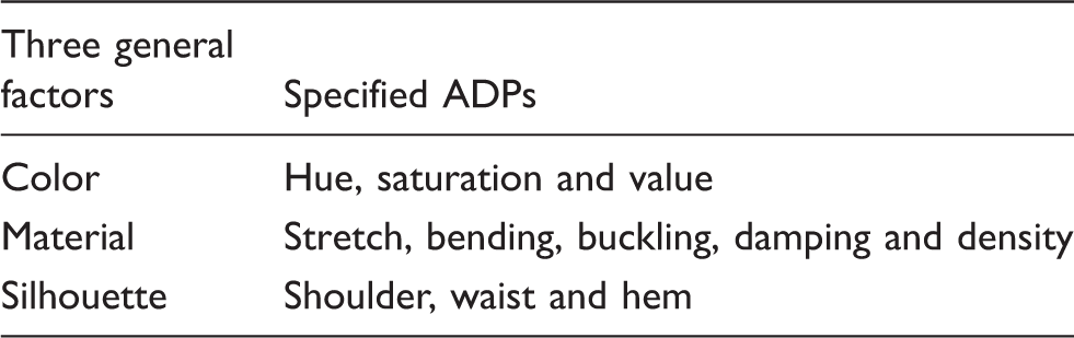
In order to address challenge 3, the selection of a proper mathematical modeling tool needs to be made. In the literature, statistical methods^12,21–25 and intelligent computing technology^26–33 have been used as a tool for this purpose. Statistical methods are used for simple and linear problems, such as regression (e.g. linear regression and logistic regression) and classification (e.g. factor analysis), while intelligent computing technology can tackle more complex and non-linear problems (e.g. artificial neural networks), and it can also deal with problems with imprecise information (e.g. fuzzy logic).³⁴ In fact, statistical methods can be viewed as a special case of the intelligent computing technology that contains more complex analysis.

In this paper, we present a work on building a model to represent the relationship from the AWs to the DPs for apparel design by applying the neural network (NN) technique. In this model, a human’s affect is the input, and DP is the output. The contributions of the work are as follows: (1) the model as developed enables affective design for apparel; and (2) a new experience of the efficacy of NNs, especially high-order NNs, is generated.

The rest of the paper is organized as follows: the second section presents the methodology for developing the mapping from AWs to ADPs. The third section is the architecture of the neural network. The fourth section is the results and discussion. The fifth section gives a validation of the developed model through an example. The sixth section is a conclusion with some further discussion.

Model development

There are two steps in applying the artificial NN model technique: (1) generation of training data and (2) determination of the weights for a particular NN architecture.

Acquisition of training data

The general methodology is to have a test-bed on which test samples with their ADPs and AWs are exposed to human subjects for them to express their opinions on the “strength” of the link between the ADPs and AWs. The test-bed includes two software systems: (1) Marvelous Designer, which is to simulate three-dimensional (3D) apparel in terms of ADPs; and (2) FluidSurvey, which is a platform for constructing a survey. The first was used in this study for constructing a test sample (apparel) described with ADPs, as shown in Table 2, and the second was used in this study to link the test sample to AWs, as shown in Table 1. The combination of these two systems results in a survey interface to the subject, as shown in Figure 1. The left part of Figure 1 shows a picture of apparel, generated by system (1), and the right part of Figure 1 shows all AWs with five-level Likert scales (1–5), generated by system (2). In the experiment, there were in total 27 test samples (which represent 27 combinations of ADPs) generated. A note is given regarding the 27 combinations. Each ADP was considered to have three levels (high, middle and low), and the orthogonal array technique³⁵ was applied to result in 27 combinations. The duration of the survey was about two months. Each survey randomly displayed six scenarios (see https://fluidsurveys.usask.ca/s/rainzhao/) to the subject, and each scenario includes an apparel picture and 30 AWs (Figure 1 as a partial interface). There were, in total, 100 subjects recruited for this survey. The criteria for selection of subjects were as follows: (1) they must be Canadian residents and (2) their age must be in the range of 18–35.

Figure 1.

A scenario from the survey.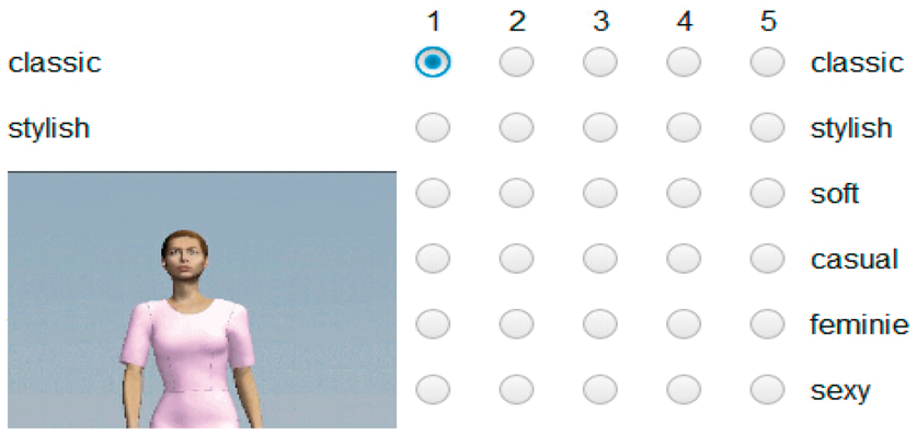

The test procedure is as follows. Step 1: a survey with a test sample (i.e. apparel picture) and AWs were shown to the subject. The survey engine thus connects ADPs and AWs. Step 2: a subject ranks the appropriate AWs he or she feels while viewing the apparel picture by use of the subjective rating scale. Step 3: a pair of “values”, namely < ADP-level, AW-scale > (e.g. ADP-level: high; AW-scale: 5), was created, and subsequently, a number of such pairs was created. In total, 600 pairs of data (i.e. training data) were created as there were 100 subjects and each subject was given six pictures.

Before performing data analysis, the data collected required some cleaning and the outliers were removed from the data. The following data were removed: (1) the same Likert item is given to all or most of the AWs (e.g. “2” is given to all AWs); (2) the difference in the Likert items to all AWs is very small (e.g. “2” or “3” is given to all AWs); (3) the data is incomplete (i.e. some items are missing).³⁶ As a result, 565 data out of 600 data were kept as the training data. The training data needs to be normalized to avoid disturbances due to different scales of data.³⁷ The data in the training data were normalized to [0, 1] with the following equation

x' = | \frac{x - x_{min}}{x_{max} - x_{min □}} |

(1)

where

x_{min □}

and

x_{max □}

are the minimum and maximum value in the value domain with respect to ADP and AW, respectively, and

x'

is the normalized value. Equation (1) is thus used for normalization for both the ADP and AW.

Neural network architecture

The NN method is a technique used to describe the multiple-input and multiple-output (MIMO) relation.^38,39 NNs consist of a set of neurons (nodes) with a set of weighted edges that connect the neurons (nodes), a set of inputs and a set of outputs (Figure 2). The layer of neurons between the input and output layers is called the hidden layer. A neuron consists of two units connected in series: (1) the unit that aggregates the weighted (denoted by w) output of neurons in the preceding layer, plus a so-called bias (denoted by b); and (2) the activated unit in which there is a mathematical function called the activated function (more discussion about the activated function will be given later in this paper). For unit (1), if the aggregated function is linear, the NN is called the linear NN; if the aggregated function is with an order more than 1 (e.g. second order), the NN is called the higher-order NN.⁴⁰

Figure 2.

The general architecture of neural networks.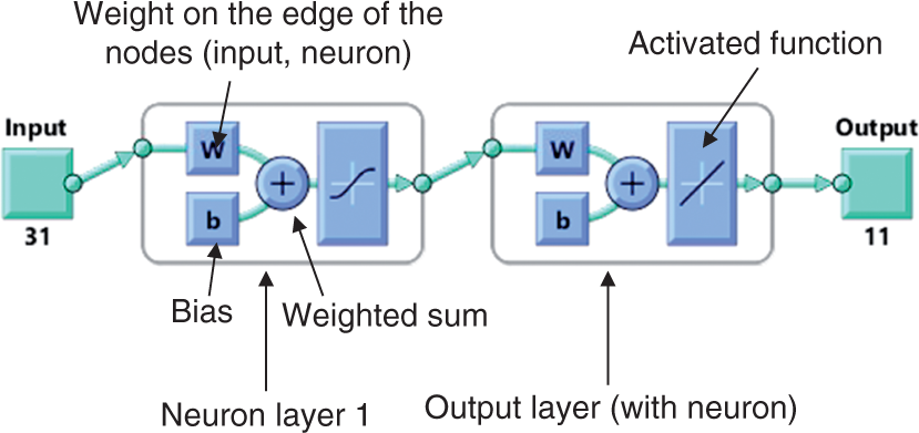

The design of a particular NN means to determine (i) the number of hidden layers, (ii) the number of neurons in each hidden layer, (iii) the activated function and (iv) the weight. Just like designing a product (e.g. apparel), the method of determining the foregoing components is empirical-based except for (iv) – determining the weight. The general principle of determining the weight is as follows: the weight is determined to make the behavior of a particular NN model under design match the known behavior of the application problem under modeling (e.g. the data pair < APA-value, AW-value>). Clearly, the known behavior of the application problem is the training data discussed previously. The process of determining the weight is called learning in the NN literature.⁴⁰ A commonly used method to determine the weight is called back-propagation (BP).⁴¹ The algorithm called Levenberg–Marquardt (LM) was used for BP in this study. The LM algorithm is available in the MATLAB NNs tool box.

There are three main types of activated functions in NNs (Figure 2), namely, the Hyperbolic Tangent Sigmoid (HTS) (or Tansig function), the Log Sigmoid (LS) (or Logsig function) and the Purlin function (or Linear function; LF).^33,42 It is noted that the rule of selecting the activated function in the output layer depends on the value range of the outputs of a particular NN architecture. If the value range of output is [0, 1], LS is chosen; if the value range is [–1, 1], HTS is chosen; and LF is suitable for both kinds of value range. In this study, we considered LS as the activated function for the output layer as the value range in the output layer in our problem is [0, 1], and considered both LS and HSL as the activated function for the hidden layers, as their value ranges are not restricted to [0, 1].

In this study, both the single hidden layer and two hidden layers of the NN architecture were attempted. Note that two hidden layer NN models are often used for solving non-linear problems.⁴³ Further, different numbers of hidden neurons were attempted, ranging from 10 to 100. In this study, 70% of the training data set (see the previous discussion) was used for training, 15% of the data was used for validation and 15% of the data was used for testing. It is noted that the purpose of validation is to minimize “over-fitting” (i.e. the sufficient number of neurons in layers). The statistic method of Mean Squared Error (MSE) was used for testing. The mathematical expression of MSE is as follows

MSE = \frac{1}{n} \sum_{i = 1}^{n} (y_{i}^{obs} - y_{i}^{pred})^{2}

(2)

where

y_{i}^{obs}

is the experimental output as observed, and

y_{i}^{pred}

is the predicted or anticipated output obtained from NNs. The smaller the MSE, the more accurate the model. R (regression coefficient) was employed to indicate the correlation between

y_{i}^{obs}

and

y_{i}^{pred}

. If R is close to 1, then

y_{i}^{pred}

is close to

y_{i}^{obs}

. In other words, the larger the R value, the better the model predicts the outcome from the data sets. Training R was obtained from the training data sets, while test R was obtained from the testing data sets. The structure of the NN models is shown in Table 3; the code for conducting the NNs can be accessed from http://homepage.usask.ca/∼yuz703/.

Table 3.

Structure for the neural network (NN) model and higher-order NN model (quadratic synaptic operation in particular)

NN parameters	NNs	High-order NNs
Numbers of layers	3 and 4	3
Numbers of hidden layer(s)	1 and 2	1
Training algorithm	Levenberg–Marquardt BP	Levenberg–Marquardt BP
Data normalization	[0, 1]	[0, 1]
Activated function (output layer)	LS	LS
Activated function (hidden layer)	LS and HTS	LS and HTS
Number of neurons	10–100	10–100
Data division	70% for training, 15% for validation and 15% for test	70% for training, 15% for validation and 15% for test
Accuracy evaluation	Test MSE of test data sets	Test MSE of test data sets
Performance evaluation	Test R	Test R

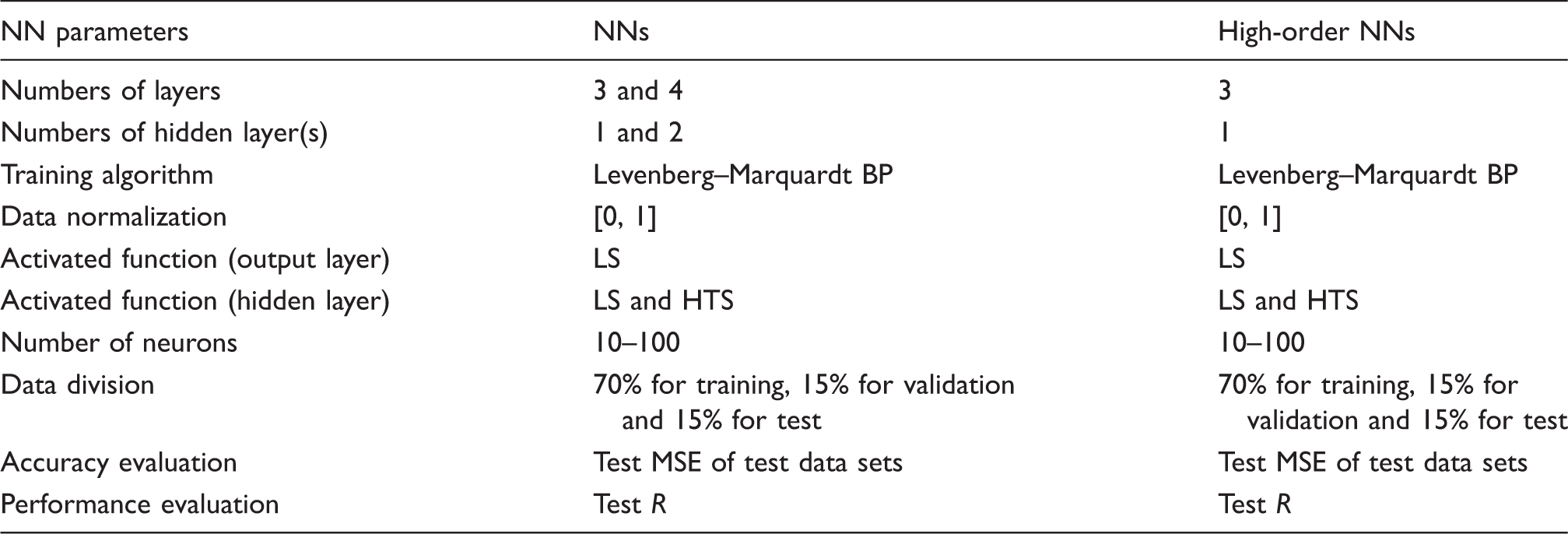
BP: back-propogation; LS: Log Sigmoid; HTS: Hyperbolic Tangent Sigmoid; MSE: Mean Squared Error.

The higher-order NN model⁴⁰ was also employed to develop the AW-to-ADP mapping in this study. In the higher-order NN model, the input to a particular neuron of a particular layer is not based on the linear weight sum but is rather the quadratic weighted function of all inputs from the preceding layer. Figure 3 shows such a NN model, which is also called Higher-order Synaptic Operation (HOSO).⁴⁰

Figure 3.

A neural unit (neuron) with the Higher-order Synaptic Operation.⁴⁰

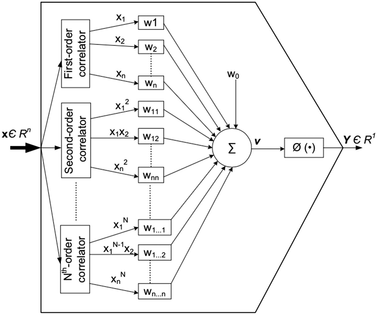
As shown in Figure 3, HOSO can be of numerous orders. The first order is the conventional linear correlation, which is the same as the conventional NNs. In this study, a second-order HOSO was considered, which is called the quadratic synaptic operation (QSO).^44–47 The Nth-order HOSO is defined as

v = w_{0} x_{0} + \sum_{i_{1} = 1}^{n} w_{i_{1}} x_{i_{1}} + \sum_{i_{1} = 1}^{n} \sum_{i_{2} = i_{1}}^{n} w_{i_{2}} x_{i_{1}} x_{i_{2}} + \dots + \sum_{i_{1} = 1}^{n} \sum_{i_{2} = i_{1}}^{n} □ \dots \sum_{i_{N} = i_{N - 1}}^{n} w_{i_{2} - i_{N}} x_{l_{1}} x_{l_{z}} \dots x_{l_{N}}

(3)

where w is the weight, x is the input and v is sum of the weighted inputs up to the second order.

In this study, the structure of the QSO was quite similar to that of the conventional NNs (Table 3). The only difference between the structure of the LSO (linear synaptic operation) and the QSO is that the LSO considered one and two hidden layers, while only a single hidden layer was considered in the QSO. It is noted that, in theory, a single-layer QSO is able to deal with non-linear problems. The code for conducting the QSO can be accessed from http://homepage.usask.ca/∼yuz703/.

Results and discussion

Forty models were built through the LSO, and twenty models were built through the QSO. Figure 4 presents a comparison for all these models in terms of MSE, in which QSO-HTS refers to the QSO with HTS as the activated function in the hidden layer, QSO-LS refers to the QSO with LS as the activated function in the hidden layer, LSO-HTS-1 refers to the LSO with a single hidden layer and with HTS as the activated function in the hidden layer, LSO-LS-1 refers to the LSO with a single hidden layer and with LS as the activated function in the hidden layer, LSO-HTS-2 refers to the LSO with two hidden layers and with HTS as the activated function in the hidden layers, and LSO-LS-2 refers to LSO with two hidden layers and with LS as the activated function in the hidden layers.

Figure 4.

Comparison of the neural network models in terms of Mean Squared Error (MSE).

It can be found from Figure 4 that the MSE of QSO-HTS and QSO-LS are more sensitive to varying numbers of neurons in the hidden layer(s) than any other LSO model. For example, the MSE of QSO-HTS dramatically changes from 10 neurons to 100 neurons. QSO-HTS hits the highest MSE (0.05664) at 20 neurons (in the hidden layer), while it hits the lowest MSE (0.03569) at 40 neurons (in the hidden layer). In general, the linear NN with two hidden layers has a better performance than the quadratic NN with one hidden layer. The smallest MSE is 0.03074 obtained from a linear NN (i.e. LSO-HTS-2 with 60 hidden neurons in the hidden layers (30 in each hidden layer, respectively)).

Figure 5 shows a comparison of the six NNs models in terms of test R. It can be found from Figure 5 that for the QSO (including both QSO-HTS and QSO-LS), the number of neurons is more sensitive than that for the LSO. For example, the test R of QSO-HTS dramatically changes from 10 neurons to 100 neurons. QSO-HTS hits the lowest test R (0.58339) at 30 neurons (in the hidden layer), while it hits the highest test R (0.71342) at 40 neurons. However, for the LSO, the number of neurons is less sensitive than that for the QSO in terms of test R. Among all the NN models, LSO-HTS-2 with 60 neurons in the hidden layers (30 neurons in each hidden layer, respectively) has the highest test R (with 0.74659) (i.e. the best prediction performance).

Figure 5.

Comparison of the neural network models in terms of test R.

From Figures 4 and 5, it can be seen that the results based on the MSE and test R are consistent. The number of neurons in the hidden layer is more sensitive with test R than that with the MSE. This is reasonable, as according to the constructs of the MSE and test R, the MSE seems to be more robust than test R. It can also be found that the quadratic NN models are more sensitive to the number of neurons than the linear NN model. This is perhaps because the quadratic NN model is less robust due to its construction.

From both Figure 4 (in terms of the MSE) and Figure 5 (in terms of test R), the mapping of the linear NNs with two hidden layers (60 neurons in total) shows a better prediction performance than that of the quadratic NN with one hidden layer (40 neurons in total). There are two reasons for this outcome. Firstly, the suitability of a particular NN model inherently depends on the characteristic of an application problem – the linear NN model with two hidden layers of neurons and quadratic NN model with one hidden layer of neurons in particular. Secondly, the fitting or approximating power of the former is higher than that of the latter, as in the former, three layers (two hidden layers and the output layer) have an activated function that is non-linear and thus contributes to the fitting or approximating power significantly. Indeed, the result herein is significant in that it provides a counter-argument to the view that a higher-order NN model is promising in terms of fewer neurons in the model for achieving the same accuracy with its counterpart (i.e. the linear NN model).⁴⁰ It is noted that the number of neurons in total in the latter (40 neurons) is indeed less than that in the former (60 neurons), but the loss of accuracy with the latter seems to be significant (MSE = 0.03 for the former, MSE = 0.04 for the latter).

Model validation

In this section, an experiment was described to validate the developed model (i.e. the AW-to-ADP mapping). The general approach to do this validation was to develop a test-bed in which the customers will comment on a particular apparel. The customers will first specify their desired affects with the AWs (shown in Table 1) and then the AW-to-ADP mapping is applied to generate an apparel for the customers (respectively). Finally, the customers will comment on whether the designed apparel meets their desired affects.

In particular, in this test-bed, four nurses were invited to participate in the experiment. The criteria for recruiting the nurses are as follows: (1) the participating nurses must be working in a Canadian hospital; and (2) the age of the participating nurses is from 20 to 40. Each of them was asked to fill out a questionnaire regarding the nurse scrub (Figure 6). The questionnaire contained 30 AWs with the five-level Likert scale. The four nurses were asked to describe their desired affects of the nurse scrub under design. In total, there were four sets of data for AWs. Table 4 shows one set of AWs, and all four sets of AWs can be found from the following web site: http://homepage.usask.ca/∼yuz703/. The next step was to use each set of AWs as the input for the AW-to-ADP mapping to obtain the ADPs, respectively. At this point, the NN model of LSO-HST-2 with 60 neurons (30 neurons in each hidden layer) was used, as it the best model (see the previous discussion). Four sets of ADPs were generated from the LSO-HST-2 model, and four nursing scrubs based on the ADPs were created with the Marvelous Designer software. Figure 7 shows one of the four scrubs, and all four scrubs can be found on the web site: http://homepage.usask.ca/∼yuz703/. The four scrubs were then shown to the participating nurses for their feedback on whether the scrubs meet their affective requirements. The feedback on the scrubs includes the degree of satisfaction regarding color, material, shoulder design, waist design, hem design and overall design of scrubs.

Figure 6.

Existing nursing scrubs in Canada.⁴⁷

Table 4.

A set of affective words (AWs) and their rank by a nurse

AW	Rank	AW	Rank	AW	Rank
Androgynous	3	Bohemian	2	Boyish	2
Casual	4	Classic	3	Comfortable	5
Conservative	4	Delicate	2	Dramatic	1
Cute	3	Edgy	2	Exclusive	3
Feminine	4	Glamorous	3	Playful	2
Practical	5	Professional	5	Romantic	1
Sexy	1	Slouchy	1	Soft	5
Sophisticated	4	Sporty	4	Stylish	4
Trendy	4	Unconventional		Understated	3
Unique	5	Vibrant	5	Youthful	5

Figure 7.

An example of a nursing scrub created by Marvelous Designer.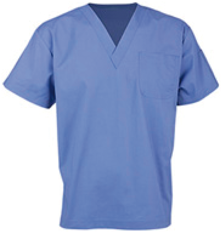

As a result of the experiment, all the nurses were satisfied with the color of the scrubs, 75% were satisfied with the material, 75% were satisfied with the shoulder design, 75% were satisfied with the waist design, 75% were satisfied with the hem design and all the nurses were satisfied with the overall design of the scrubs for their own desired affects.

Conclusions

In this paper, the development of the AW-to-ADP mapping, especially the mapping from AWs to ADPs, was presented. The mapping allows for affective design, namely given a set of desired AWs, one can find ADPs by use of the mapping. The technique used to develop the mapping was NNs. Both conventional NNs and higher-order NNs (in particular, linear NNs with one and two hidden layers and quadratic NNs with one hidden layer) were used to develop the mapping. A sufficient number of training data were acquired and the NNs were trained. The accuracy of the NN models was evaluated by the MSE and test R. The number of neurons for the hidden layers was determined with the tool available in the NN toolbox of MATLAB. A case study to show the validity of the mapping was also conducted. The following conclusions can be drawn from the results: (1) the mapping based on the architecture of the linear NN with two hidden layers is better than the mapping based on the architecture of the quadratic NN with one hidden layer in terms of both the MSE and test R; (2) the mapping makes sense for affective design for apparel products.

It is noted that in the literature, work closely relevant to the study presented in this paper may refer to the Kawabata evaluation system (KES).¹⁶ However, there are two major differences between the KES and our work. Firstly, the KES only considered the comfort feeling of the customer given a fabric material property, while our work considered a list of 30 AWs, which is obtained through a comprehensive data mining technique.¹⁷ Secondly, the KES can only be used for analysis (i.e. from ADPs to AWs), while our work targets design (i.e. from AWs to ADPs).

There are several limitations with the development described in this paper. The first limitation is that the number of training data is still restricted (about 600 in this case); ideally, 1000 training data may be better to test the number of neurons from 10 to 100. The second limitation is that the number of hidden layers for the quadratic NN model is only one; in the future, the quadratic NN with two hidden layers may be considered. Such a study will help us to understand further the characteristics of higher-order NNs in comparison with linear NNs to applications.

Footnotes

Declaration of conflicting interests

The authors declared no potential conflicts of interest with respect to the research, authorship, and/or publication of this article.

Funding

The authors received no financial support for the research, authorship, and/or publication of this article.

References

Wang

et al.

Object-oriented templates for automated assembly planning of complex products. IEEE Trans Autom Sci Eng 2014; 11: 492–503.

. Engineering informatics: state of the art and future trends. Front Eng Manag 2014; 1: 277–288.

Wang

et al.

AutoAssem: an automated assembly planning system for complex products. IEEE Trans Ind Inform 2012; 8: 669–678.

Wang

. Parameter mapping and data transformation for engineering application integration. Inform Syst Front 2008; 10: 589–600.

et al.

A decision support system for product design in concurrent engineering. Decis Support Syst 2007; 42: 2029–2042.

et al.

A polychromatic sets approach to the conceptual design of machine tools. Int J Prod Res 2005; 43: 2397–2421.

Chen

. An object-oriented intelligent CAD system for ceramic kiln. Knowl Base Syst 2001; 14: 263–270.

Zhang WJ and Werff K van der. A critique of conceptual data modeling, notions relative to the machine design domain. In: Proceedings of the 1994 ASME engineering database symposium' 94, Minneapolis, USA, 11–14 September 1994, pp.59–66. New York, NY, USA: American Society of Mechanical Engineers.

Lin

Zhang

. Integrated design of function, usability, and aesthetics for automobile interiors: state of the art, challenges, and solutions. Proc Inst Mech Eng I J Syst Contr Eng 2006; 220: 697–708.

10.

McCann J, Hurford R and Martin A. A design process for the development of innovative smart clothing that addresses end-user needs from technical, functional, aesthetic and cultural view points. In: Proceedings of the ninth IEEE international symposium on wearable computers, Osaka, Japan, 18 October 2005. Los Alamitos: IEEE Computer Soc.

11.

Gupta

. Design and engineering of functional clothing. Ind J Fibre Text Res 2001; 36: 327–327.

12.

Moody

Kinderman

Sinha

. An exploratory study: relationships between trying on clothing, mood, emotion, personality and clothing preference. J Fashion Market Manag 2010; 14: 161–179.

13.

. Fashion design styles recommended by consumers' sensibility and emotion. Hum Fact Ergon Manuf Serv Ind 2009; 19: 158–167.

14.

Khalid

Helander

. Customer emotional needs in product design. Concurr Eng 2006; 14: 197–206.

15.

Cho

Lee

. Development of a macroscopic model on recent fashion trends on the basis of consumer emotion. Int J Consum Stud 2005; 29: 17–33.

16.

Shishoo

. Importance of mechanical and physical properties of fabrics in the clothing manufacturing process. Int J Clothing Sci Technol 1995; 7: 35–42.

17.

Zhao Y, Montazeri A, Wang C, et al. On development of methods for expressing customer affective response for apparel products. In: Proceedings of. CAD’15, London, UK, 2010, pp.315–320. UK: Taylor & Francis.

18.

Schwarz

Cowan

Beatty

. An experimental comparison of RGB, YIQ, LAB, HSV, and opponent color models. ACM Trans Graph (TOG) 1987; 6: 123–158.

19.

Mahar

Ajiki

Dhingra

et al.

Fabric mechanical and physical properties relevant to clothing manufacture: -part 3: shape formation in tailoring. Int J Clothing Sci Technol 1989; 1: 6–13.

20.

Charfi

Gagalowicz

Brun

. Measurement of viscosity damping parameters of fabric related to a non-linear textile model. Text Res J 2006; 76: 787–798.

21.

Chae

Black

Heitmeyer

. Pre-purchase and post-purchase satisfaction and fashion involvement of female tennis wear consumers. Int J Consum Stud 2006; 30: 25–33.

22.

North

De Vos

Kotze

. The importance of apparel product attributes for female buyers. J Fam Ecol Consum Sci 2003; 31: 41–51.

23.

Ayada

Miki

Niwa

. Discriminating the silhouette of ladies’ garments based on fabric mechnical properties. Int J Clothing Sci Technol 1991; 3: 18–27.

24.

Lowe

Dunsing

. Clothing satisfaction determinants. Home Econ Res J 1981; 9: 363–373.

25.

Niwa

Nakanishi

Ayada

et al.

Optimum silhouette design for ladies' garments based on the mechanical properties of a fabric. Text Res J 1998; 68: 578–588.

26.

Kim SJ, Kim EY, Jeong K, et al. Emotion-based textile indexing using colors, texture and patterns. In: International symposium on visual computing. Berlin Heidelberg: Springer, 6 November 2006, pp.9–18.

27.

Wong

Yeung

et al.

Neural network predictions of human psychological perceptions of clothing sensory comfort. Text Res J 2003; 73: 31–37.

28.

Gong

Chen

. Predicting the performance of fabrics in garment manufacturing with artificial neural networks. Text Res J 1991; 69: 477–482.

29.

Fan

Newton

et al.

Predicting garment drape with a fuzzy-neural network. Text Res J 2001; 71: 605–608.

30.

Liang

Gao

. An integrated approach for agricultural ecosystem management. IEEE Trans Syst Man Cybern C Appl Rev 2008; 38: 590–599.

31.

Duan

. Business intelligence for enterprise systems: a survey. IEEE Trans Ind Inform 2012; 8: 679–687.

32.

Shi

Huang

et al.

MSMiner—a developing platform for OLAP. Decis Support Syst 2007; 42: 2016–2028.

33.

Feng

. An intelligent decision support system for fuzzy comprehensive evaluation of urban development. Exp Syst Appl 1999; 16: 21–32.

34.

Cai

Lin

Han

et al.

On a simple and efficient approach to probability distribution function aggregation. IEEE Trans Syst Man Cybern Syst 2016; 99: 1–100.

35.

IBM. SPSS conjoint 22, http://library.uvm.edu/services/statistics/SPSS22Manuals/IBM%20SPSS%20Conjoint.pdf (2015, accessed 27 July 2015).

36.

Li Q, Ma ZM and Zhang WJ. Modeling of incomplete information and uncertain information in database for engineering design and production management. In: ASME 12th engineering information management symposium, Atlanta, GA, USA, 13–16 September 1998, Paper number: DETC98/EIM-5686, New York, NY, USA: American Society of Mechanical Engineers.

37.

Sola

Sevilla

. Importance of input data normalization for the application of neural networks to complex industrial problems. IEEE Trans Nuclear Sci 1997; 44: 1464–1468.

38.

Zhou

. A variational approach to intensity approximation for remote sensing images using dynamic neural networks. Exp Syst 2003; 20: 163–170.

39.

Zhou

. A new type of recurrent fuzzy neural network for modeling dynamic systems. Knowl Base Syst 2001; 14: 243–251.

40.

Gupta

Jin

Homma

. Static and dynamic neural networks: From fundamentals to advanced theory, 1st ed. Hoboken, NJ: Wiley–IEEE Press, 2003.

41.

Heaton

. Introduction to neural networks for C#, Washington DC: Heaton Research, Inc., IBM SPSS, 2008.

42.

Alavala

. Fuzzy logic and neural networks, New Delhi, India: New Age International, 2008.

43.

Lapedes

Farber

. Nonlinear signal processing using neural networks: Prediction and system modelling, USA: IEEE, 1987.

44.

Gupta

Rao

. Neuro-control systems-theory and applications, USA: IEEE Neural Networks Council, 1993.

45.

Gupta MM. Correlative type higher-order neural units with applications. In: Proceedings of the IEEE international conference on automation and logistics (ICAL), Qingdao, China, 8–10 December 2008, pp.715–718. USA: IEEE.

46.

Gupta

Homma

Hou

et al.

Higher order neural networks: fundamentals theory and applications. In: Zhang

(ed). Artificial higher-order neural networks for computer science and engineering: Trends for emerging applications, Hoboken, NJ: Information Science Reference, 2010, pp. 397–422.

47.

Medical Scrubs. Wishing Well Medical, https://wishingwellmedicalsupply.com/medical-scrubs-los-angeles/ (2015, accessed 8 July 2015).