Toward three-dimensional modeling of the interaction between the air flow and a clamped–free yarn inside the main nozzle of an air jet loom

Abstract

In air jet looms, the weft yarn is transported from the prewinder to the reed by means of an air flow. In this work, the motion of a yarn inside a main nozzle during the first stage of an insertion process is modeled and analyzed. In this stage, the weft yarn is clamped at one side and free at the other side. Therefore, the deformation waves of a clamped–free yarn are modeled. A three-dimensional, two-way, fluid–structure interaction simulation has been performed in which the yarn is represented as a flexible cylinder and the arbitrary Lagrangian–Eulerian technique is employed. The results of the simulation have been compared quantitatively and qualitatively with experiments. It was, however, not possible to match the initial position and stress state of the yarn in the simulations to that in the experiments. This causes large differences between the simulated and measured yarn positions and wave characteristics, especially at the beginning. The agreement between experimental and simulated wave characteristics notably improves as time progresses, but substantial differences remain. Analyzing the overall motion of the yarn inside the main nozzle shows that the mixing region, where the shocks are located, can be considered as an excitation point. In this point, the aerodynamic normal forces are high if the yarn is not located on the axis of the main nozzle. All deformation waves start from the mixing region and propagate along the yarn.

Keywords

weft yarn insertion main nozzle fluid–structure interaction clamped–free dynamic mesh deformation waves

The air jet loom is widespread in the textile industry due to its high productivity. In air jet looms, the weft yarn is transported from the prewinder to the reed by means of an air flow. In the first stage of the insertion, the weft yarn is fixed or clamped by a magnetic pin and an air flow is built up in the main nozzle. The second stage starts by releasing the weft yarn, which then accelerates by means of aerodynamic forces. In the reed, the weft yarn speed is kept constant by relay nozzles. When the weft yarn reaches the end of the reed, it is brought to a halt and cut off. Subsequently, the reed is moved so as to push the weft against the cloth.

The main nozzle is mainly designed to generate axial forces on the weft yarn. However, due to the effect of gravity, the weft yarn deviates from the axis of the nozzle, giving rise to normal forces due to shocks and turbulence. The normal forces deform the weft yarn and these deformations propagate inside the main nozzle, affecting both the yarn and the air flow.

Although modeling the motion of yarns in air flows has attracted many researchers’ interest, most of the published works ignored the interactions between air flows and yarns. For example, in Uno,¹ Uno et al.,² Adanur and Mohamed,^3,4 Turel et al.,⁵ Adanur and Turel,⁶ Celik et al.⁷ and Nosraty et al.,⁸ no air flow simulations were carried out. The air flow quantities were obtained based on simplified equations or experiments. These works were aimed at calculating the yarn speed or the yarn tension or to study the effects of yarn motion on the performance of air jet looms. Other research focused on developing numerical models to model yarn motion, for example, the one-dimensional model suggested by Vangheluwe et al.,⁹ De Meulemeester et al.¹⁰ and Yamamoto and Matsuoka,¹¹ or the three-dimensional (3D) model developed by De Meulemeester et al.¹² However, the air flow–yarn interactions were also not taken into account. Nevertheless, the works^1–12 helped one to understand the dynamic behavior of yarns, led to improved performance of air jet looms and provided numerical models to predict the motion of yarns.

The development of computational fluid dynamics (CFD) and computational structure dynamics provided powerful tools to carry out air flow–yarn interaction simulations. For example, Cai and Oxenham¹³ performed one-way fluid–structure interaction (FSI) simulations of air flow–fiber in the fiber transfer channel of a rotor spinning machine. They calculated the air flow with a CFD software package and transferred the resultant velocity and pressure to a fiber movement model. They showed the effectiveness of using numerical tools to study the dynamics of fibers in textile processes. Zeng et al.¹⁴ performed two-way and two-dimensional FSI simulations of a fiber in high-speed air flow. They represented the fiber as beads connected by massless rods; the air flow was laminar and incompressible. The effect of the fiber motion on the air flow was taken into account by a source term. They applied their models to simulate fiber motion in the nozzle of an air jet spinning machine. However, they mentioned that the proposed procedure was computationally very expensive. Tang and Advani¹⁵ and Kondora and Asendrych¹⁶ modeled the motion of fibers by representing the fiber as a chain of spheres connected by ball and socket joints. Zeng et al.¹⁷ and Sun et al.¹⁸ modeled fiber whipping motion (bending deformations) during the process of melt blowing by performing two-way FSI simulations. They derived a structure equation for a flexible fiber, represented as connected beads, and coupled it with a flow solver. Pei and Yu^19,20 modeled the motion of a fabric in the vortex spinning nozzle. They performed two-way FSI simulations using an arbitrary Lagrangian–Eulerian (ALE) technique in which the mesh is dynamic. The air flow was incompressible and turbulent and the domains of the simulations were two-dimensional and planar. They studied the effects of some geometrical parameters of the nozzle, the inlet pressure and the yarn delivery speed on the dynamic behavior of a cotton fabric and found good agreement between their results and experiments. Zhu and Chin²¹ modeled the motion of flexible elastic filaments in a viscous pulsatile flow using the immersed boundary method. Battocchio et al.²² suggested a two-dimensional multi-body dynamics model to simulate the dynamics of a long polymeric fiber in a high-speed turbulent flow. They used the Articulated-Body algorithm to model the fiber motion, which consisted of a chain of rigid rods. Pei et al.²³ modeled the dynamics of a ramie yarn hair by performing two-way FSI simulations. They used the same procedure as presented by Pei and Yu,^19,20 but considered the air flow to be compressible. Wu et al.²⁴ carried out two-dimensional, two-way FSI simulations to analyze deformations of a weft yarn during the start-up stage in an air jet loom. They employed the ALE technique and took into account the pressure effects, but ignored the viscous forces. They compared the results of the simulations with photos taken by a high-speed camera during experiments.

This paper continues the work done by Osman et al.²⁵ on modeling and analyzing the dynamic behavior of yarns during the insertion process of an air jet loom. In that work, the motion of a weft yarn during one complete insertion was modeled by means of FSI simulations of air flow–yarn. The fluid model was two-dimensional axisymmetric, the structure model was 3D and the ALE technique was not used. The fluid mesh was static and the effect of the yarn motion on the air flow was modeled by adding a source term. The idea of this work is to study the motion of a weft yarn during the insertion process by means of completely 3D two-way FSI simulations with the ALE technique. In our previous work, some simplifications were made to carry out the FSI simulations. However, performing the two-way FSI simulations in a 3D configuration, as presented in this paper, increases the cost and duration of the simulations. In this research, only the motion of a yarn during the first stage of the insertion is modeled and analyzed, with the yarn clamped at one end and free at the other end. This avoids complications related to the axial motion of the yarn. As the forces on the yarn are strongly dependent on its position, being able to simulate the yarn motion during the clamped part of the insertion is an important first step into simulating the entire insertion process. Furthermore, this research aims at providing insight into the problems and possibilities of using 3D FSI simulations for weft yarn insertion. The results of the simulations are compared quantitatively and qualitatively to experiments. Some of the works mentioned above, for example Pei and Yu,^19,20 also performed two-way FSI simulations with the ALE technique. However, the domains of the simulations were two-dimensional in those works to avoid the complexity of 3D two-way FSI simulations with moving grids. Consequently, the presented work is a significant improvement compared to the state of the art. It should be noted that a smooth mono-filament yarn is used for the current work as this reduces uncertainty on the surface and structural properties of the yarn. The proposed simulation methodology could be applied to any type of yarn, provided that a good structural model is available for the yarn and that one can model the influence of the yarn’s surface structure.

Experimental details

The numerical simulations are set up according to a case that has been investigated experimentally. In the experiment, the deformations of a clamped–free yarn were recorded by a high-speed camera in a main nozzle made of glass. The camera type is Kodak Ekta Pro EM. The image capture rate was adjusted to 10,000 frames per second to capture clearly the motion of the yarn. The yarn is a nylon 6.6 mono-filament and its properties, according to measurements, are as follows: the diameter is 0.72 mm, the yarn linear density is 464 tex and the Young’s modulus (E) is 2.5 GPa. The yarn is clamped at the yarn inlet of the main nozzle and is free at the exit of the tube.

At the beginning of the experiment, the main nozzle is supplied with a pressure of 0.14 bar (all pressures are relative to the atmospheric pressure), creating a holding flow that keeps the yarn more or less on the axis of the main nozzle. Afterwards, the supply pressure is increased to 5 bar. There is a tube between the compressed air tank and the main nozzle, but the pressure at the inlet of the main nozzle is measured during the experiment. The pressure was sampled at a frequency of 10 kHz using a piezo-resistive pressure transducer with a least count of 0.046 bar (Meggitt model 8530B, 200 psia range). Figure 1 shows the measured pressure profile at the inlet of the main nozzle. The initial pressure corresponds to the pressure of the holding flow, equal to 0.14 bar. After 5.4 ms, a valve is opened and the pressure increases sharply to 5.35 bar. This value is higher than the inlet pressure, which is equal to 5 bar. This higher value is due to pressure waves traveling between the tank and the inlet of the main nozzle. From 18 to 57 ms, the pressure varies between 4 and 5 bar. Afterwards, the pressure reduces back to 0.14 bar.

Figure 1.

Measured pressure profile at the inlet of the main nozzle during the experiment. The values are relative to the atmospheric pressure.

A schematic diagram of the experimental setup is provided in Figure 2. The camera records the motion of the yarn in a vertical plane. The motion is recorded, separately, in two parts of the nozzle tube as the high-speed camera cannot capture the entire tube at once with sufficient resolution. The holding flow is already present at the beginning of the video recordings. This can be observed in Figure 1 in which the measured pressure at zero time (the beginning of the recordings) corresponds to the holding flow pressure.

Figure 2.

Experimental setup.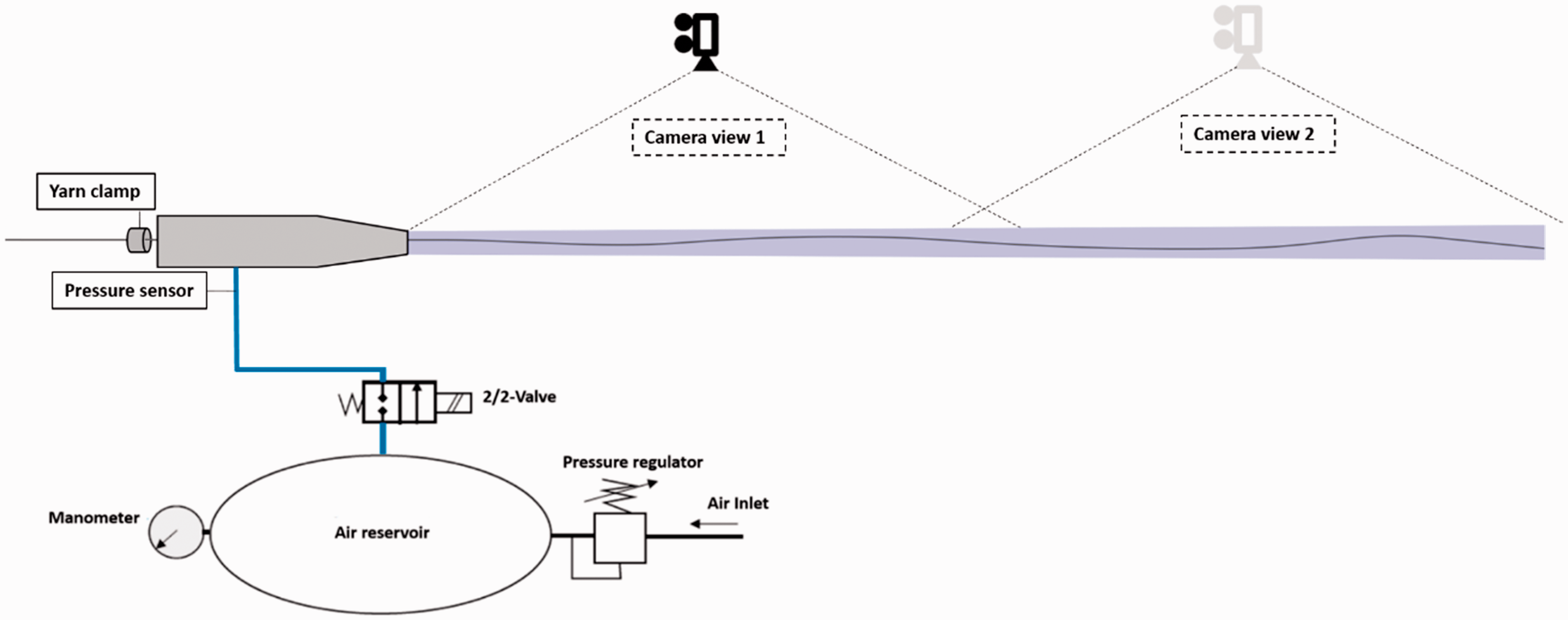

A meridional section of the geometry of the main nozzle, used in the experiment, is depicted in Figure 3 with the main dimensions indicated.

Figure 3.

Meridional view of the geometry of the main nozzle. The red, black and blue lines represent the nozzle body, the needle and the tube, respectively. (Color online only.)

Simulation setup

Flow solver

The computational fluid domain, which is 3D, consists of the main nozzle geometry and two additional outer zones, as shown in Figure 4(a). The yarn is represented as a cylinder with diameter equal to the yarn diameter of 0.72 mm. The cylinder extends from the yarn inlet to the end of the main nozzle tube. The yarn is clamped at the yarn inlet, as shown in Figure 4(a). At the exit of the tube, the yarn is free. The mesh is structured, as can be seen in Figure 4(b), and contains about 367,000 cells. The mesh is gradually refined toward the mixing region to more accurately capture the shocks. A somewhat higher mesh density has also been incorporated at the tube outlet. The coordinate system is shown in Figure 4(a); the origin is located at the yarn inlet.

Figure 4.

(a) Meridional view of the computational fluid domain with the boundary conditions. (b) Details of the mesh.

Figure 5 displays the static pressure as calculated on the yarn if it is fixed on the axis with an inlet pressure of 5 bar. Two different meshes are used with 367,000 cells and 735,000 cells, respectively.

Figure 5.

Static pressure on yarn, obtained from simulation with yarn fixed on the axis. Mesh 2 contains approximately double the number of cells of mesh 1.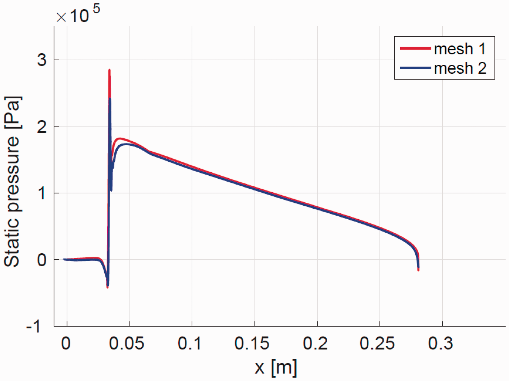

From Figure 5 it can be seen that the mixing region is most sensitive to mesh refinement. However, performing calculations on the finer mesh would drastically increase the computational time. Since the deviation remains quite limited, it is not expected to affect the general conclusions.

As the mesh is dynamic, the ALE formulation of the flow equations is solved (Donea et al.²⁶ and Sanches and Coda²⁷). The air flow is compressible and turbulent; the shear stress transport k–ω model (k–ω SST) (Menter²⁸) is used as the turbulence model.

The 3D transient simulations of the air flow have been performed using Ansys Fluent 17.0, in which the coupled scheme is used as the solution method for pressure and velocity. The second-order upwind scheme is used for the convective terms in the density, momentum and energy equations. The least-squares cell-based method is used for the gradients. The second-order implicit scheme is used for the time discretization.

Several methods can be used to handle the dynamic mesh. The smoothing method is applicable to a structured and an unstructured mesh and is employed in this work. The principle of the smoothing method is to distribute the displacements of the fluid–structure interface over the cells from the surrounding fluid domain. The Laplacian (diffusion) technique is used in this work for the extension of the grid displacements. This technique is based on the Laplace equation to calculate the new positions of the grid nodes.

The boundary conditions are set as follows: the inlet pressure is set equal to the measured pressure profile shown in Figure 1. The outlet pressure is set to atmospheric pressure. The wall of the needle, tube and yarn are set to no-slip walls.

As mentioned above, at the beginning of the experiment the holding flow is already present. Therefore, at the beginning of the FSI simulation the initial values of the air flow quantities correspond to the values obtained with 0.14 bar inlet pressure. The yarn’s initial position is on the axis of the main nozzle. The convergence tolerances are set to 10⁻⁶ for all flow quantities. The time step used for the flow simulations equals 5 × 10⁻⁶s and 3400 time steps are carried out.

Structure solver

The structural computational domain is shown in Figure 6. It consists of the yarn as a cylinder and the tube of the nozzle (which is called the fictive tube, as will be explained in the next paragraph). The cylinder’s length is 0.28 m. The structured mesh of the cylinder contains 4800 elements of type C3D20R. C stands for continuum elements, which are used for solid analysis, 3D means 3D, 20 is the number of nodes and R stands for reduced-integration, which reduces the number of integration points required to calculate the element matrices. The properties of the cylinder are set to those of the yarn, which are linear density 464 tex, Young’s modulus E = 2.5 GPa and Poisson's ratio $υ = 0.39$ . Neither displacements nor rotations are allowed at the fixed end of the yarn.

Figure 6.

Computational structural domain.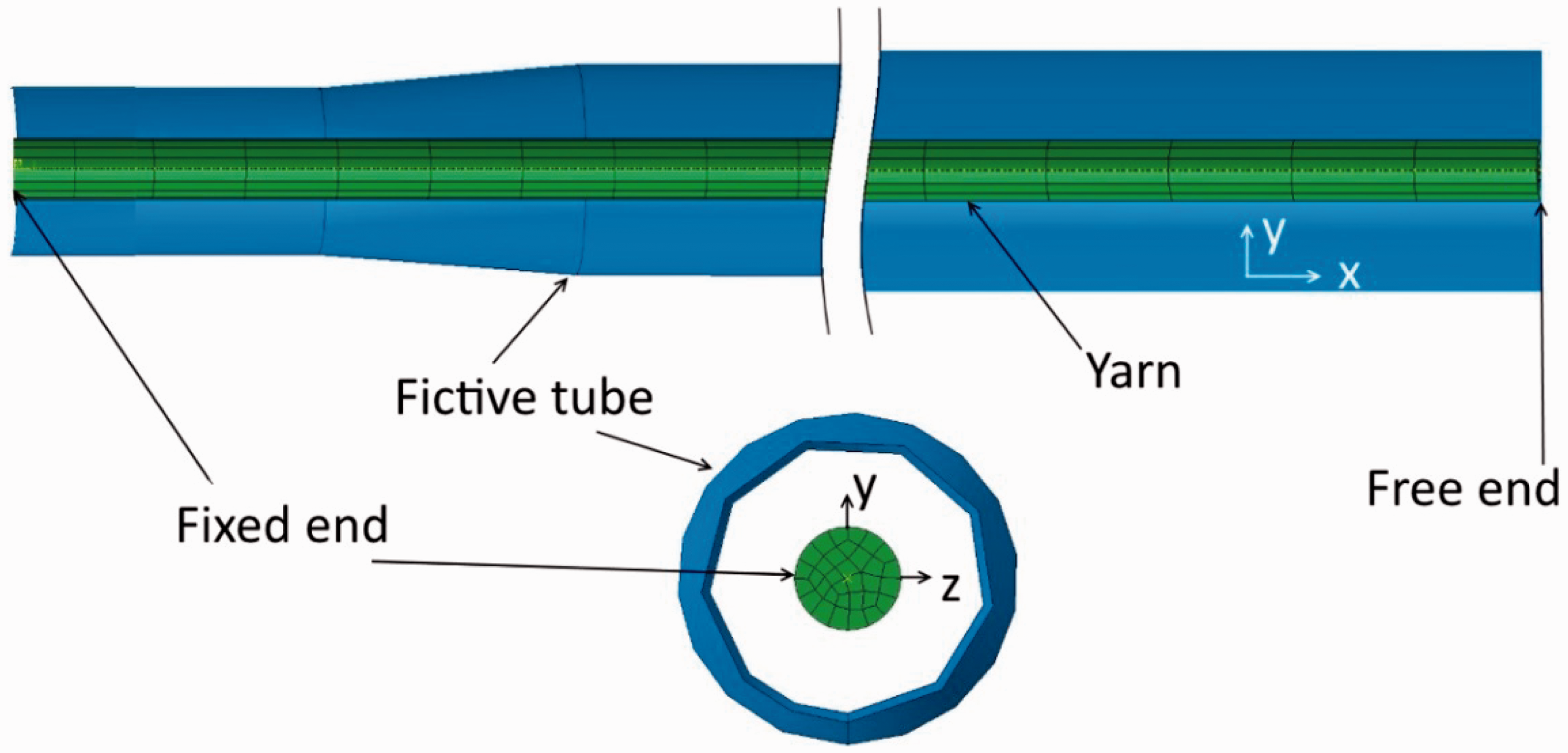

The fictive tube, shown in Figure 6, is not a meshed body, but an analytical rigid body. The idea of this body is to prevent the yarn from moving out of the main nozzle. Moreover, the radial dimensions of this fictive tube are 15% smaller than the corresponding ones from the tube in the fluid domain for dynamic mesh considerations. If the yarn came into contact with the actual tube, the fluid mesh between the yarn and the tube would be completely compressed and the simulation would crash. Therefore, the yarn motion is constrained to the fictive tube with smaller diameters, which prevents failure of the fluid dynamic mesh motion. Frictionless contact is set between the yarn and the fictive tube in the tangential direction and hard contact in the normal direction.

The equation governing the motion of a structure (the weft yarn in this case) is

ρ_{s} \frac{\partial^{2} \vec{u}}{\partial t^{2}} - \nabla \cdot {\bar{σ}}_{s} = {\bar{f}}_{s}

(1)

where

ρ_{s}

is the density of the weft yarn,

\vec{u}

is the deformation of the weft yarn,

{\bar{f}}_{s}

is the body force per unit volume and

{\bar{σ}}_{s}

is the stress tensor. Equation (1) is discretized with the finite element method. The Hilber–Hughes–Taylor implicit time integration method is used. The geometrical nonlinearity is taken into account. In addition to the fluid loads, which are pressure and viscous traction, gravity is also included in the structure calculations. The 3D structural implicit dynamics have been calculated using Abaqus 6.14 (Simulia Inc., Providence, RI, USA). The time step that is used in the structural simulation is the same as the one used in the flow simulation (

Δ t = 5 \times 10^{- 6} s

Coupling algorithm

The FSI simulation has been performed with two separate codes. The air flow calculations are strongly or implicitly coupled with the structural calculations and the interface Quasi-Newton technique with an approximation of the inverse of the Jacobian from a least-squares model (IQN-ILS) has been used (Degroote et al.²⁹). With an implicit coupling algorithm, the coupling equilibrium conditions on the fluid–structure interface are satisfied in each time step. These equilibrium conditions are the kinematic equilibrium $\vec{v} = \frac{d \vec{u}}{dt}$ and the dynamic equilibrium ${\bar{σ}}_{f} \cdot {\vec{n}}_{f} = - {\bar{σ}}_{s} \cdot {\vec{n}}_{s}$ , where $\vec{v}$ is the air flow velocity, $\vec{n}$ is the unit normal pointing outwards and the subscripts f and s refer to the fluid and the structure, respectively.

The relative convergence tolerance is set to 10⁻⁶ with a maximum number of 20 coupling iterations allowed. However, after a few time steps, three coupling iterations were sufficient to reach the imposed convergence tolerance.

Results and discussion

Comparison with the experiment

To validate the results of the simulations, they are compared to the experiments. It should be mentioned that the initial position of the yarn is not the same in the simulations as it is in the experiments. Although it is possible to impose an initial deformation in the simulations, obtaining the initial yarn position from the video recordings is not feasible since only part of the yarn could be recorded at once. Furthermore, extracting the position of the yarn in three dimensions would require synchronized footage from a second camera angle. In addition, inaccuracies in the extracted yarn position, small deviations in the nozzle geometry or small variations in local yarn properties can result in a notably different yarn position after some time. Moreover, the stress components along the yarn cannot be obtained from the video footage, prohibiting a complete description of the yarn’s initial state.

Figure 7 shows the positions of the yarn in three frames for both the simulation and the experiment. In the simulations, the initial position of the yarn is on the axis of the main nozzle. From Figure 7(a) it can be seen that the yarn in the first frame of the simulation is still positioned almost perfectly on the axis of the main nozzle. The video recordings show that from 0 to 5 ms the yarn position remains basically unaltered. This implies that from 0 to 5 ms, the air flow simply holds the yarn in the same position. Therefore, it can be stated that the response of the yarn to the air flow is the same in the experiment and in the simulation during the first 5 ms. The difference is just in the initial position of the yarn.

Figure 7.

Frames of the yarn during experiments and the corresponding frames of the simulations at time: (a) 5 ms; (b) 12 ms; (c) 15 ms. The domain shown starts from the needle tip to 130 mm downstream. Images are vertically enlarged by a factor 2. The tube border is highlighted in blue and the yarn (edge) is highlighted in green. (Color online only.)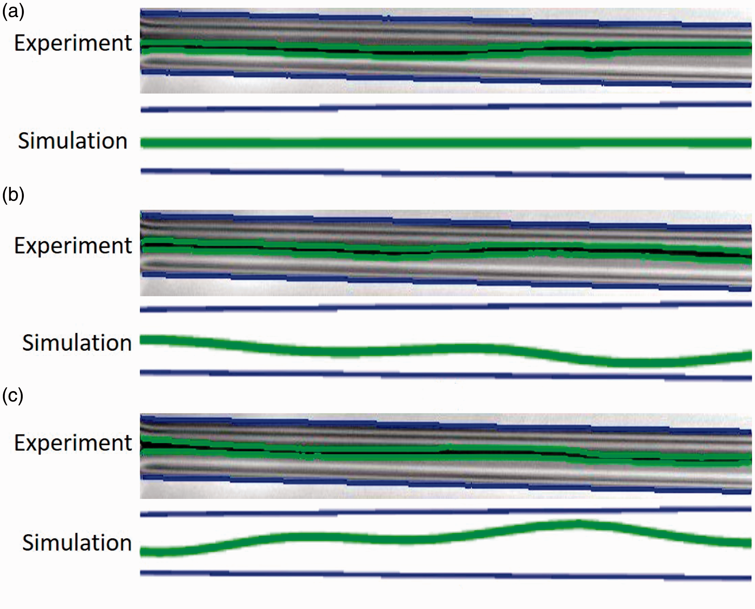

The different initial position of the yarn in the simulation with regard to the experiment affects the subsequent positions. Figure 7(b) and (c) display the deformations observed during the experiment and the simulation at a later time. These deformations run along the yarn. Comparing exactly the position of the yarn in Figure 7(b) and (c) is not meaningful because of several reasons. First, the initial position is not the same in the simulations and the experiments. Second, local variations in the real yarn properties cannot be taken into account in the simulations but can influence the yarn position.

Figure 8 shows three frames of the yarn position in the second half of the tube. Figure 8(a) shows the position of the yarn at 5 ms. Also in this part of the tube, the position of the yarn has not changed from the beginning of the video recordings up to 5 ms. Increasing the inlet pressure of the nozzle forces the yarn to move back to the axis of the main nozzle, as shown in Figure 8(b). Then, the deformation waves move along the yarn, as can be seen in Figure 8(c).

Figure 8.

Frames of the yarn during experiments and the corresponding frames of the simulations at time: (a) 5 ms; (b) 12 ms; (c) 15 ms. The length of the shown domain equals 125 mm; the right-hand side of the domain shown is at the tube exit. Images are vertically enlarged by a factor 2. The tube border is highlighted in blue and the yarn (edge) is highlighted in green. (Color online only.)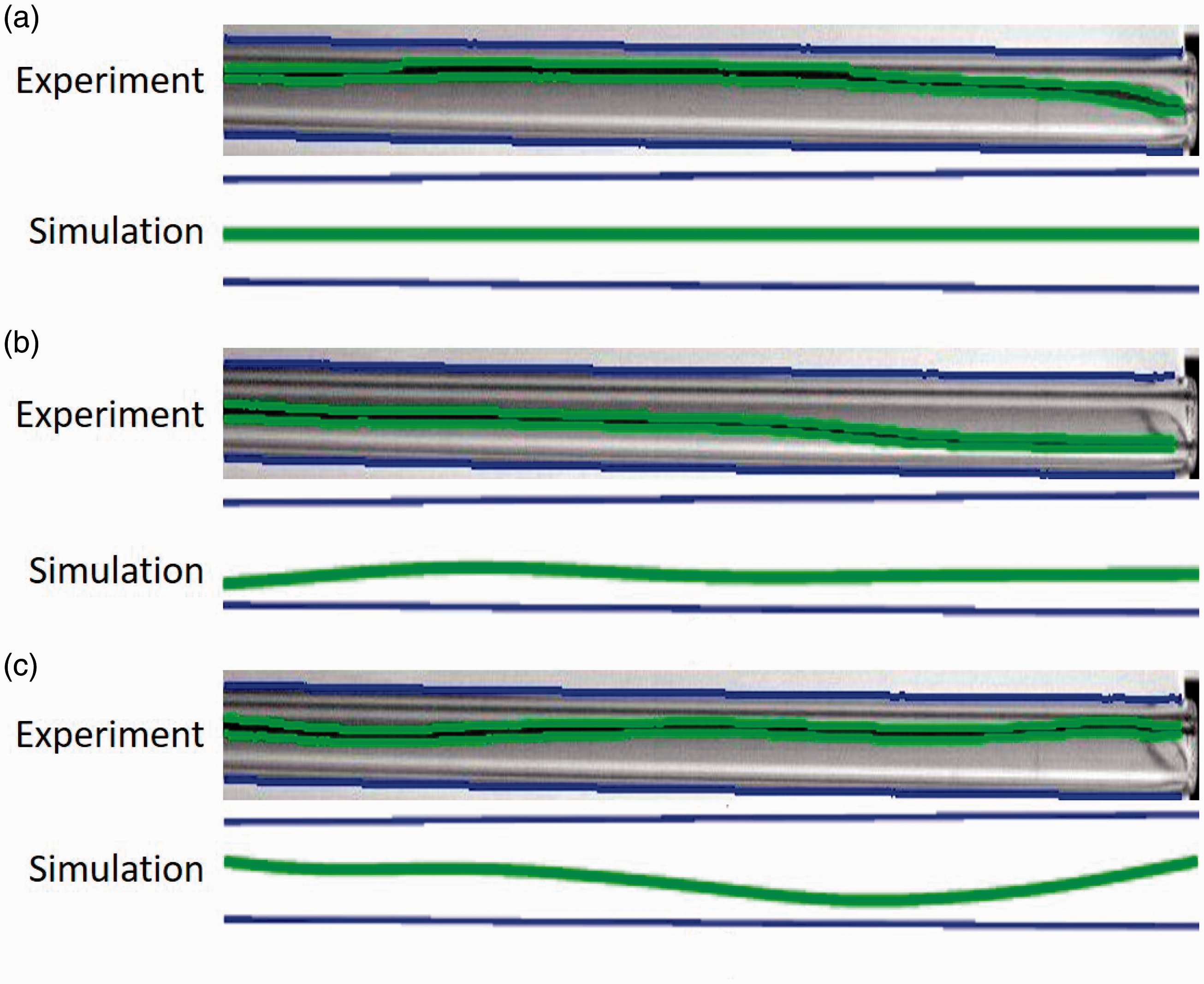

Comparing the mode shapes of the deformation waves in Figures 7 and 8 has not given a clear conclusion about the results of the simulations. Therefore, the wave length and speed are considered.

The characteristics of the waves are measured and calculated, as shown in Figure 9. A point from a wave is chosen to be followed; that point has to be either a crest or a trough. For example, in Figure 9 point A from the chosen wave is followed and the wave speed is calculated according to $c = Δ x_{A} / Δ t$ with $Δ x_{A} {= x}_{A_{, frame 2}} - x_{A_{, frame 1}}$ and $Δ {t = t}_{frame 2} - t_{frame 1}$ . The wave length (λ) is taken directly from the frame, as shown in Figure 9. In the same way, three waves are measured from the video recordings and the results are listed in Table 1.

Figure 9.

Wave characteristics and measurement. Point A from the shown wave is followed to calculate the wave speed.

Table 1.

Measured waves from the experiment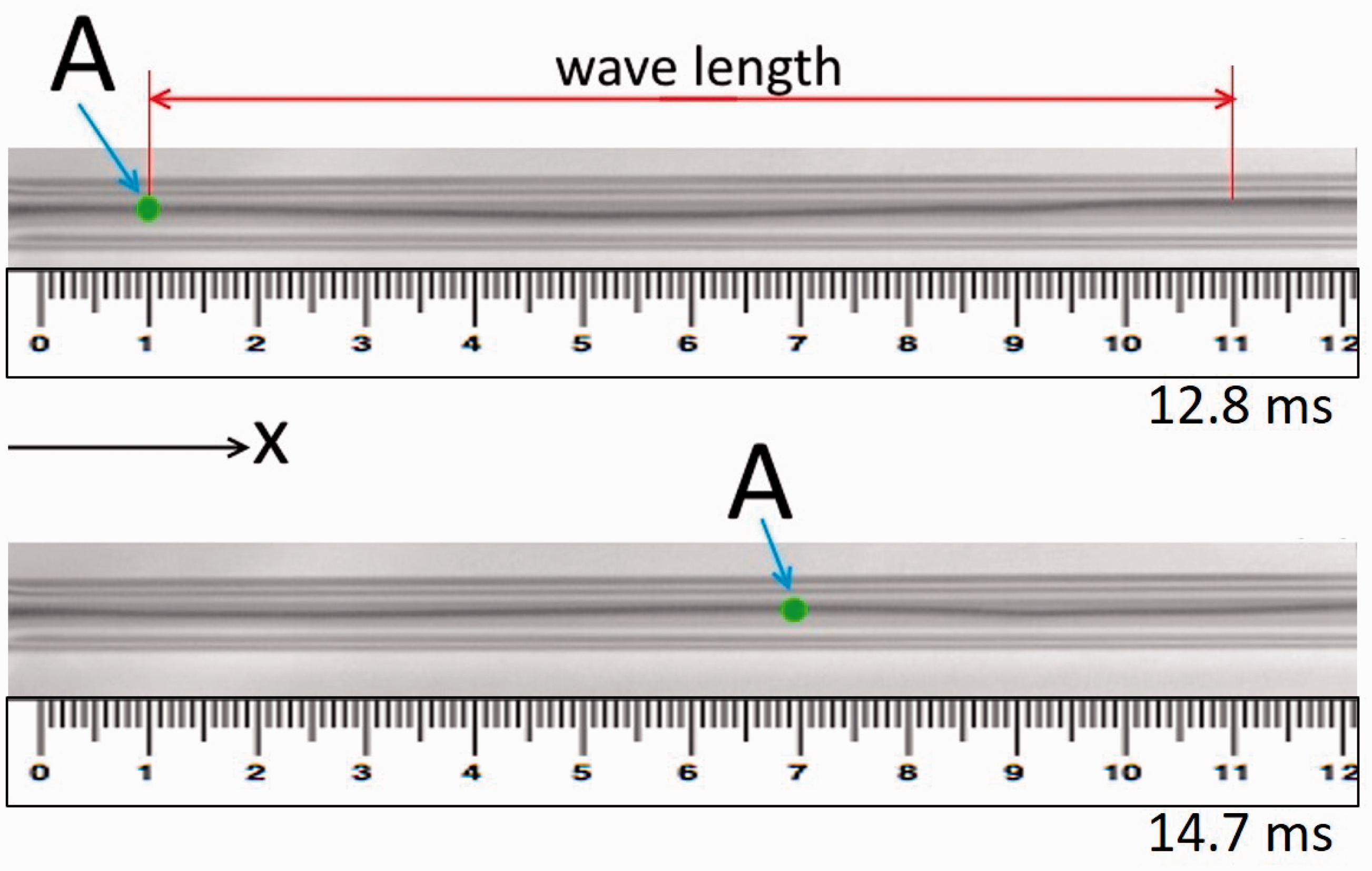

Wave	Frame time [ms]	c [m/s]	_λ [mm]
1	7.8–10.4	15.3	70.0
2	12.8–14.7	31.5	100.0
3	15.4–16.6	33.3	80.0

Table 2 lists the obtained values of the wave characteristics from the simulations and the differences compared to those from the experiment. For the first wave the difference is 61% for the wave speed, but for the second and the third wave the differences decrease to 6% for the wave speed. It should be mentioned that the experimental values are only a crude estimate, as measuring and calculating the waves from the video recordings is quite challenging.

Table 2.

Calculated waves from the simulation. The percentage values are the deviations from the corresponding experimental values

Wave	Frame time [ms]	c [m/s]	_λ [mm]
1	8.5–9.9	39.5 (+61.2%)	48.0 (−48.8%)
2	10.6–11.8	38.3 (+17.7%)	91.0 (−9.9%)
3	14.6–16.2	35.6 (+6.4%)	60.0 (−33.3%)

The difference in mode shapes between the simulation and the experiment, which are seen in Figures 7 and 8, are due to the differences in the wave lengths and speeds. As the differences decrease with time, it can be postulated that the different initial position of the yarn in the simulation and the experiment causes these differences. In fact, at the beginning of the simulation, the yarn is positioned on the axis of the main nozzle, while the initial position of the yarn in the experiment cannot be imposed or controlled and is only approximately positioned on the axis by the holding flow. Based on the discussion above it can be stated that the different initial position causes large differences in wave characteristics for the first deformation wave. For subsequent deformation waves, the obtained wave speeds are within acceptable accuracy (between 6.4% and 17.7% difference) of the experimental values.

Yarn motion

The overall motion of the yarn is analyzed based only on the results of the simulation. Although the correspondence between experiment and simulation when comparing the yarn position is rather poor, the simulations can still provide valuable clues about the mechanisms behind the yarn deformation.

Three points from the yarn centerline are chosen. By plotting the coordinates of the three points, it can be observed how the deformations propagate along the yarn. The selected points are located in the mixing zone (see Figure 4), in the middle of the tube and at the yarn’s free end. Initially, the points are positioned on the axis at respectively 35.3, 158.4 and 283.0 mm from the yarn inlet. Figure 10 shows the y- and z-coordinates of the three points during the simulations.

Figure 10.

Coordinates of three points from the yarn centerline during the simulations: (a) y-coordinates; (b) z-coordinates. (Color online only.)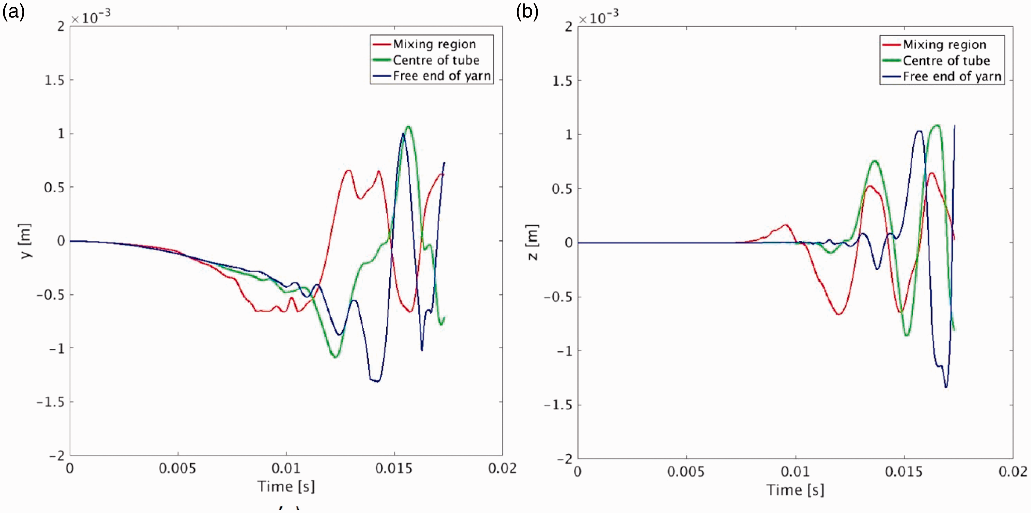

Figure 10(a) shows that, in the first 7 ms of the simulation, the yarn falls toward the tube bottom due to gravity. Moreover, Figure 10 indicates that, for example, at 5 ms, the y-coordinates of the three points are almost the same and the same holds for the z-coordinates. Figure 11 displays frames of the yarn centerline in the xy- and xz-planes. Note that the scale in Figure 11(b) is smaller than the scale in Figure 11(a). In Figure 11(a) it can be seen that the yarn falls due to gravity, but deformation waves with low amplitudes are also present. As the yarn falls, it does not experience a symmetrical flow anymore and, thus, normal forces are generated due to pressure differences. All deformations start in the mixing zone and propagate downstream.

Figure 11.

Frames of the yarn centerline: (a) y-coordinates; (b) z-coordinates.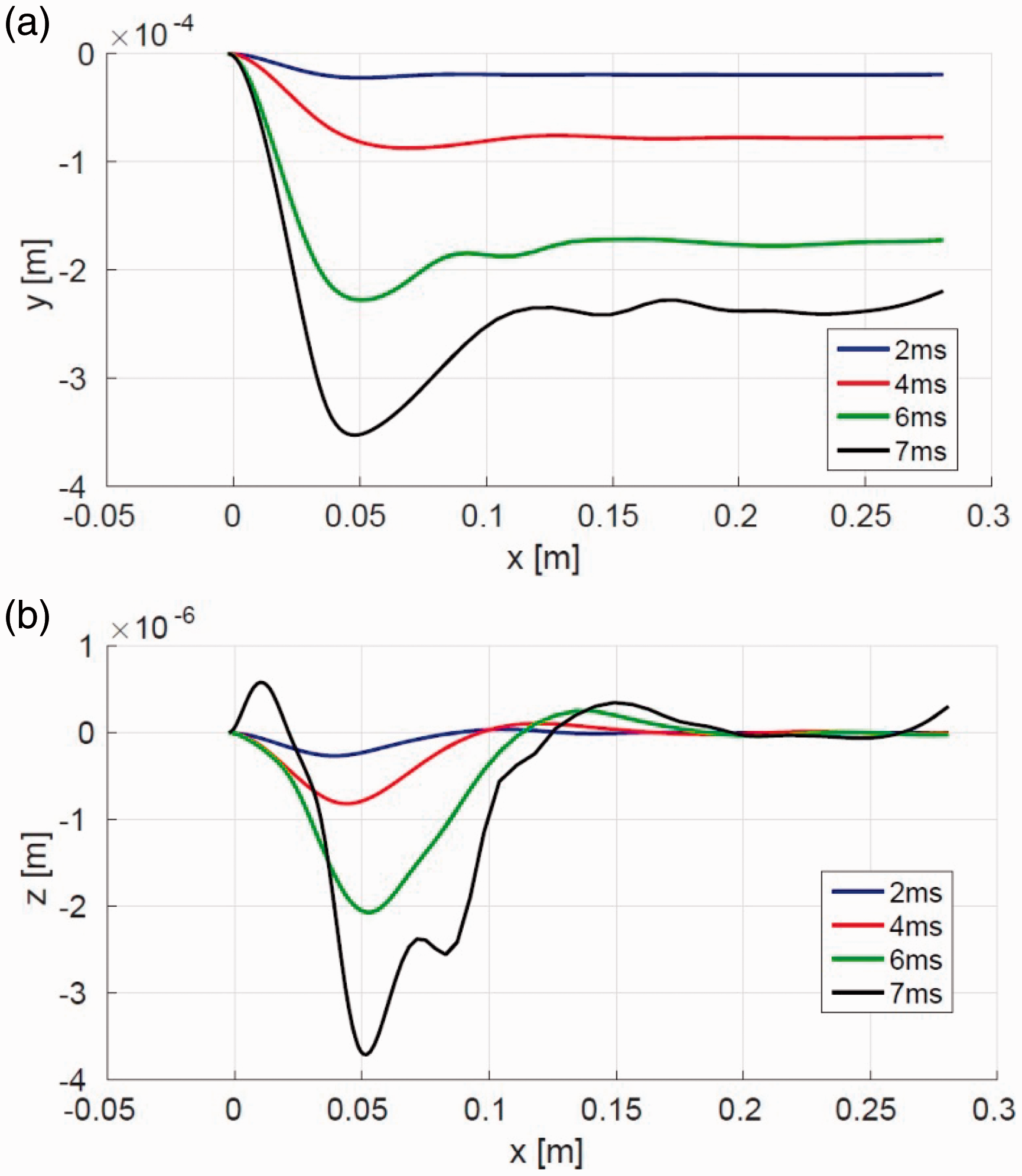

After 10 ms of simulation time, the amplitudes of the waves increase along z and y directions, as seen in Figure 10. The wave amplitudes increase due to an increase of the inlet pressure (see Figure 1), which increases the aerodynamic forces on the yarn wall. Figure 12 shows contours of static pressure in the yz-plane at an axial coordinate equal to the coordinate of the point in the mixing region (red color line in Figure 10). The static pressure around the yarn in Figure 12 can be divided into two regions: a region with high values of static pressure and another with low values. The yarn is pushed toward the region of low pressure.

Figure 12.

Contours of static pressure in the yz-plane at an axial coordinate located in the mixing zone, at time: (a) 11.5 ms; (b) 12 ms.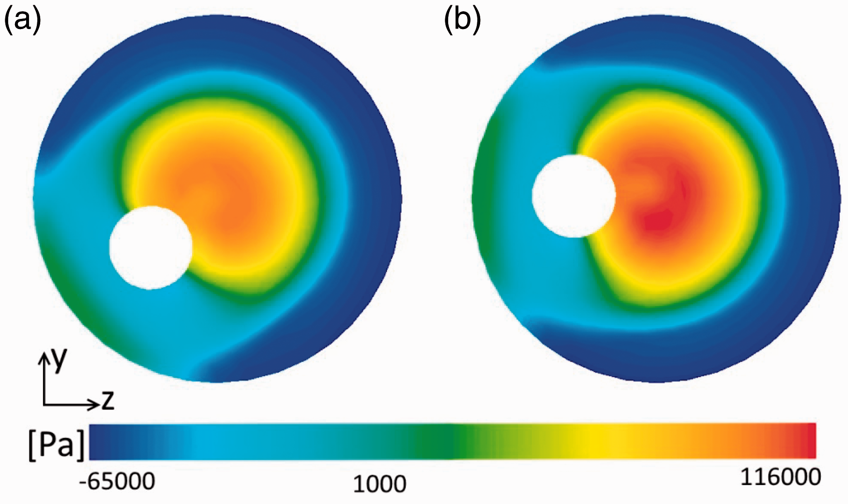

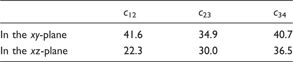
Figure 13 shows four other frames of the yarn centerline at a later time than the frames in Figure 11. It can be seen that the amplitudes of these waves are higher than the ones in Figure 11. The numbers that are highlighted in Figure 13 show the same crest of a wave. This wave or crest propagates inside the tube. Therefore, the speed of the wave can be calculated based on this crest. The calculated wave speeds are listed in Table 3.

Figure 13.

Frames of the yarn centerline in the xy- and xz-planes. The highlighted numbers show the location of the same crest of a wave in the four frames.

Table 3.

Speed of the waves shown in Figure 13 [m/s]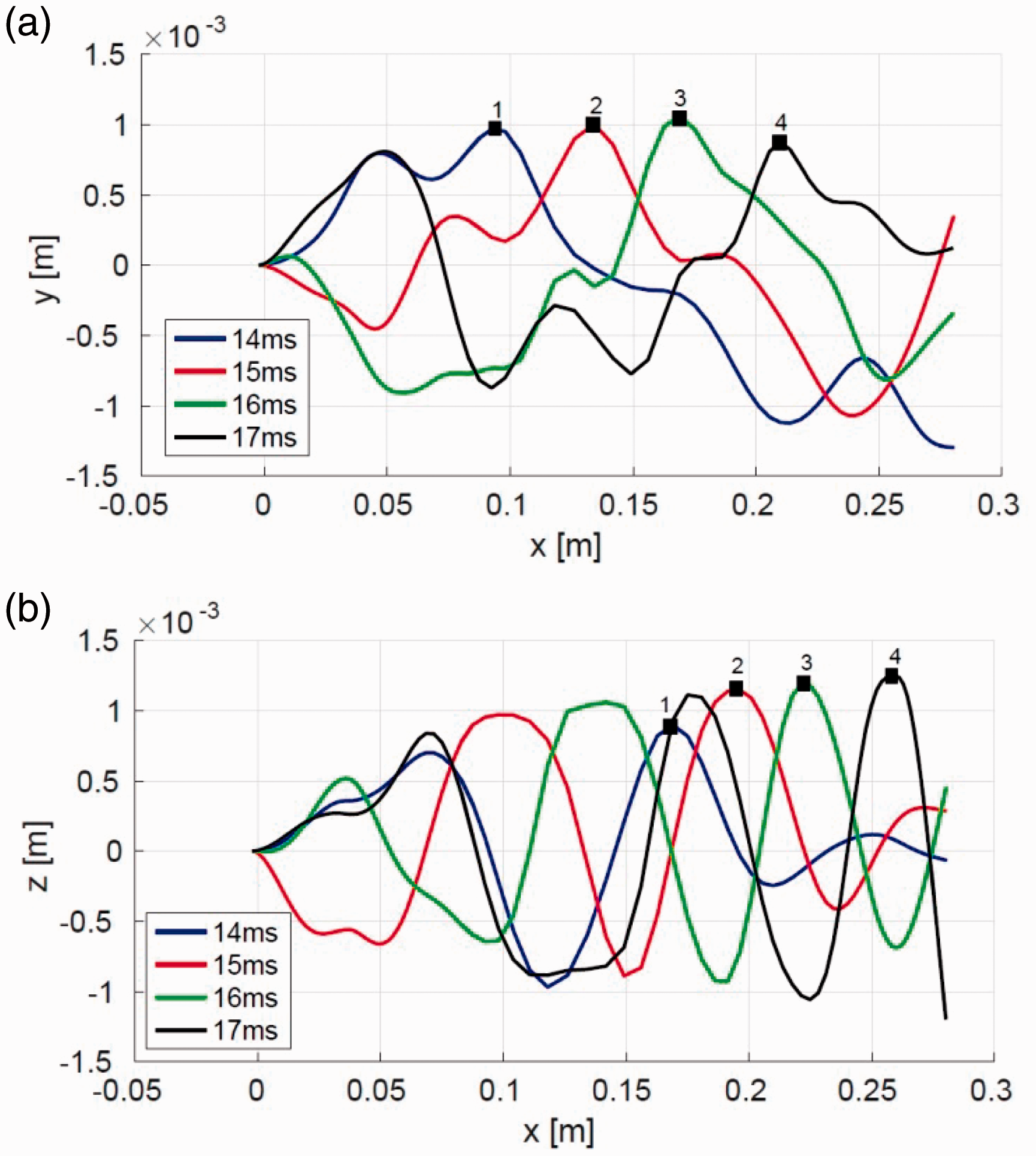

	c ₁₂	c ₂₃	c ₃₄
In the xy-plane	41.6	34.9	40.7
In the xz-plane	22.3	30.0	36.5

The results of the FSI simulation, shown in Figures 11 and 13, indicate that the deformation waves start from the mixing region where the shocks are located. There, the yarn is subjected to strong normal pressure forces if, locally, it is not perfectly aligned with the axis.

Figure 14 shows two frames of the yarn position and the associated y-components of the viscous and pressure force. Figure 14(b) shows that the contributions of the viscous force in the vertical direction are small. The y-component of the force depends mainly on the pressure, as shown in Figure 14(c). It can be seen that there are large contributions in the mixing region where the shocks are located.

Figure 14.

(a) Yarn centerline position in the xy-plane. (b) Y-component of viscous force along the yarn centerline. (c) Y-component of pressure force along the yarn centerline.

Figure 15 shows the contours of the Mach number. It can be seen how the Mach number changes around the mixing region due to the effects of shocks, expansion and compression waves. This is not the case in another part of the tube, for example in Figure 15(b).

Figure 15.

Contours of Mach number in the xy-plane at 13 ms: (a) around the mixing region; (b) between x = 175 and 190 mm.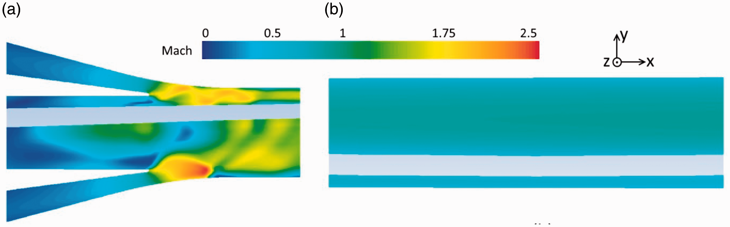

It can be concluded that if the yarn is not on the axis of the main nozzle, it is subjected to normal forces generated by the effects of the shocks. The normal forces deform the yarn and the deformation waves run along the yarn. Therefore, the location of the shock can be considered as an excitation point. The deformation waves can be linked to the pressure force in this excitation point. Stronger shocks result in higher pressure forces, which result in larger deformations.

Conclusion

In this paper, the FSI simulation of air flow–yarn inside a main nozzle has been presented. The domains of the simulation are 3D and the ALE technique has been employed. The first stage of an insertion process has been modeled. In this stage, the yarn is clamped on one side and it is free on the other side. The weft yarn is represented as a cylinder in the simulations. The deformation waves that run along the yarn have been obtained and analyzed.

The results of the simulation have been compared with video recordings of the yarn motion during the experiments. The initial state of the yarn is not the same in the simulation and the experiment. Therefore, large differences between the simulation and the experiment have been observed. However, as time progresses and the influence of the initial state diminishes, acceptable wave speeds (between 6.4% and 17.7% difference with experiments) are retrieved.

By analyzing the global motion of the yarn it could be concluded that the deformation waves start from the mixing region and propagate along the yarn. These deformations result from the presence of the shocks, which cause a force away from the centerline if the yarn is not perfectly aligned with it. The contribution of the viscous forces to the radial motion is negligible compared to the effect of the pressure forces.

Footnotes

Declaration of conflicting interests

The authors declared no potential conflicts of interest with respect to the research, authorship, and/or publication of this article.

Funding

The authors disclosed receipt of the following financial support for the research, authorship, and/or publication of this article: This work was financially sponsored by Aleppo University of Syria, by a Starting Grant from the Special Research Fund of Ghent University and by the Flemish government agency for Innovation by Science and Technology (IWT), project number 120519.

References

Uno

. A study on an air-jet loom with sub-streams added, part 1: deriving the equation of motion for weft. J Text Mach Soc Jpn 1972; 18: 37–44.

Uno

Shiomi

Kise

. A study on an air-jet loom with sub-streams added, part 2: analysis of various weaving factors by the equation of motion of weft. J Text Mach Soc Jpn 1972; 18: 86–92.

Adanur

Mohamed

. Analysis of yarn motion in single-nozzle air-jet filling insertion, part I: theoretical models for yarn motion. J Text Inst 1992; 83: 45–55.

Adanur

Mohamed

. Analysis of yarn tension in air-jet filling insertion. Text Res J 1991; 61: 259–266.

Turel

Bakhtiyarov

Adanur

. Effects of air and yarn characteristics in air-jet filling insertion, part I: air velocity and air pressure measurements. Text Res J 2004; 74: 592–597.

Adanur

Turel

. Effects of air and yarn characteristics in air-jet filling insertion, part II: yarn velocity measurements with a profiled reed. Text Res J 2004; 74: 657–661.

Celik

Babaarslan

Bandara

MPU

. A mathematical model for numerical simulation of weft insertion on an air-jet weaving machine. Text Res J 2004; 74: 236–240.

Nosraty

Jeddi

AAA

Mousalloo

. Simulation analysis of weft yarn motion in single nozzle air-jet loom to study the effective parameters. Indian J Fibre Text Res 2008; 33: 45–51.

Vangheluwe

Sleeckx

Kiekens

. Numerical simulation model for optimisation of weft insertion on projectile and rapier looms. Mechatronics 1995; 5: 183–195.

10.

De Meulemeester

Githaiga

Van Langenhove

et al.

Simulation of the dynamic yarn behavior on airjet looms. Text Res J 2005; 75: 724–730.

11.

Yamamoto

Matsuoka

. A method for dynamic simulation of rigid and flexible fibers in a flow field. J Chem Phys 1993; 98: 644–650.

12.

De Meulemeester

Puissant

Van Langenhove

. Three-dimensional simulation of the dynamic yarn behaviour on air-jet looms. Text Res J 2009; 79: 1706–1714.

13.

Cai

Oxenham

. Computer modeling of fiber movements in high-speed airflow. RJTA 2005; 9: 77–85.

14.

Zeng

Yang

. Mixed Euler-Lagrange approach to modeling fiber motion in high speed air flow. Appl Math Model 2005; 29: 253–261.

15.

Tang

Advani

. Dynamic simulation of long flexible fibers in shear flow. CMES 2005; 8: 165–176.

16.

Kondora

Asendrych

. Modelling the dynamics of flexibles and rigid fibres. Chem Process Eng Inz 2013; 34: 87–100.

17.

Zeng

Sun

Wang

. Numerical approach to modeling fiber motion during melt blowing. J Appl Polym Sci 2011; 119: 2112–2123.

18.

Sun

Zeng

Wang

. Three-dimensional model of whipping motion in the processing of microfibers. Ind Eng Chem Res 2011; 50: 1099–1109.

19.

Pei

. Numerical study on the effect of nozzle pressure and yarn delivery speed on the fiber motion in the nozzle of Murata vortex spinning. J Fluids Struct 2011; 27: 121–133.

20.

Pei

. Investigation on the dynamic behavior of the fiber in the vortex spinning nozzle and effects of some nozzle structure parameters. J Eng Fibers Fabr 2011; 6: 16–29.

21.

Zhu

Chin

RCY

. Simulation of elastic filaments interacting with a viscous pulsatile flow. Comput Meth Appl Mech Eng 2008; 197: 2265–2274.

22.

Battocchio F, Sutcliffe MPF and Teschner F. Dynamic simulation of long polymeric fibres immersed in a turbulent air flow. In: Eberhard P and Ziegler P (eds) proceedings of the IMSD2012 - the 2nd joint international conference on multibody system dynamics, Stuttgart, Germany, 29 May–1 June 2012, http://www2.eng.cam.ac.uk/~mpfs/papers/BST2012FibreTurbulentIMSD.pdf.

23.

Pei

Chen

Mao

et al.

Dynamics of the ramie yarn hair in the nozzle of the jetwind process and effects of some nozzle parameters. J Nat Fibers 2015; 12: 430–443.

24.

Chen

Liu

et al.

Air-flow characteristics and yarn whipping during start-up stage of air-jet weft insertion. Text Res J 2016; 86: 1988–1999.

25.

Osman A, Malengier B, De Meulemeester S, et al. Simulation of air flow-yarn interaction inside the main nozzle of an air jet loom. Text Res J. 2018; 88: 1173–1183.

26.

Donea

Giuliani

Halleux

. An arbitrary Lagrangian-Eulerian finite element method for transient dynamic fluid-structure interactions. Comput Meth Appl Mech Eng 1982; 33: 689–723.

27.

Sanches

RAK

Coda

. On fluid-shell coupling using an arbitrary Lagrangian-Eulerian fluid solver coupled to a positional Lagrangian shell solver. Appl Math Model 2014; 38: 3401–3418.

28.

Menter

. 2-equation eddy-viscosity turbulence models for engineering applications. AIAA 1994; 32: 1598–1605.

29.

Degroote

Bathe

K-J

Vierendeels

. Performance of a new partitioned procedure versus a monolithic procedure in fluid–structure interaction. Comput Struct 2009; 87: 793–801.