Models for basic warp knitted fabrics Part II: single guide bar fabrics (closed-lap and open-lap)

Abstract

Warp knitted fabrics are mainly used as household goods, technical textiles, medical textiles, etc. Modeling of these fabrics is necessary for predicting the desired technical or medical functions beforehand. In this context, the present series of papers is devoted to the modeling of basic warp knitted fabrics. In this, Part II of this series, models for single guide bar fabrics are created. There are mainly two types of single bar fabrics, namely closed-lap and open-lap single bar fabrics. Structures are also changed by having different lapping movements up to the five needle spaces. In this work, 1 and 1, 2 and 1, 3 and 1, 4 and 1 closed-lap and 1 and 1, 2 and 1, 3 and 1 open-lap single bar warp knitted fabrics are considered.

During modeling, the loop leanings in the course-wise direction are considered, curvature equalities at the loop parts are attained as much as possible, two connected parabolas are taken as the fabric plane model of the loop connection part, loop heads are taken as parametric ellipses in two dimensions and the remaining loop parts are modeled by wrapping parabolic or cubic curves on imaginary cylindrical or conical objects. The models created are versatile and they can be changed and used for special cases.

The models created are drawn to scale by using the 3DS-MAX computer graphical program. At first glance, it is seen that the shapes obtained by the models are similar to the ones that can be observed in real samples.

Keywords

geometrical model warp knitted fabric closed-lap open-lap single bar

Single bar warp knitted fabrics are produced on a single needle bar warp knitting machine by using a single guide bar. There are mainly two types of single bar fabric structures, namely closed-lap and open-lap structures. While loop legs are crossing with each other for closed-lap structures, the legs of the loops do not cross with each other for open-lap structures. Example sketch diagrams of both the closed-lap and open-lap structures are given in Figure 1.

Figure 1.

Example sketch diagrams of single bar warp knitted fabrics: (a) 2 and 1 closed-lap single bar fabric; (b) 1 and 1 open-lap single bar fabric (Paling¹).

Loop formation is not given here as it can be found in any textbook, such as in Ray’s,² but the motions of the guide bar are important to be given here. The guide bar has two motions: (a) swinging motion through the needles forward and backward; (b) lateral motion or lapping motion, which is parallel to the needle bar. There are two lapping motions of the guide bar for one course of knitting: (i) overlap and (ii) underlap. Overlapping movement takes place when the guide bar swings to the back of the machine (or in front of the needle hooks) and mainly one needle space to the right or to the left of the machine. Underlapping movement takes place when the guide bar swings to the front of the machine. The underlap motion of the guide bar can be more than one needle space up to five needle spaces to the left or to the right-hand side of the machine. Single bar fabric structures change again according to the number of underlapping movements in front of the machine. For this reason, single bar fabrics are called the 3 and 1, the 5 and 1 single bar fabric, etc. The meaning of the 3 and 1, for example, is three needle spaces underlap and one needle space overlap, etc. Examples of lapping movements are also shown in Figures 1(a) and (b), that is, Figure 1(a) shows a sketch diagram of the 2 and 1 closed-lap single bar warp knitted fabric while Figure 1(b) shows a 1 and 1 open-lap single bar warp knitted fabric.

In single bar warp knitted fabrics, underlapping yarns are seen at the back of the fabrics.

Knitting instructions of single bar warp knitted fabrics can be given by their threading orders and their lapping movements (or chain notations) for a repeating unit, as given in Figure 2 for the closed-lap and in Figure 3 for the open-lap structures.

Figure 2.

Knit notations of closed-lap single bar warp knitted fabrics: (a) closed-chain stitch; (b) 1 and 1 closed-lap; (c) 2 and 1 closed-lap; (d) 3 and 1 closed-lap; (e) 4 and 1 closed-lap.

Figure 3.

Knitting instructions of open-lap single bar warp knitted fabrics: (a) open chain stitch; (b) 1 and 1 open-lap; (c) 2 and 1 open-lap; (d) 3 and 1 open-lap; (e) 4 and 1 open-lap.

In textile composite applications, three-dimensional and also multiaxis composite fabric reinforcements are developed. These composite reinforcement fabrics can be based on woven, weft knitted, braiding or warp knitted fabric structures (see Bilişik et al.³ and Bilişik⁴). For multiaxis composite reinforcement fabrics, high-performance yarns or rovings are inserted in a textile structure in different directions starting from the fabric length direction: 0, 90, ±45 degree angles. The inserted yarns carry the applied loads in their extending directions. Inserted yarns should be as straight as possible in the structure. The best results are obtained by inserting the high-performance yarns in the single bar warp knitted fabric structures. Therefore, multiaxis composite reinforcements are developed in the base of single bar warp knitted fabrics (see Ray² and Bilişik et al.³). Figure 4 shows multiaxis composite reinforcement fabrics stitched with 1 and 1 single bar warp knitted fabrics.

Figure 4.

Sketch diagrams of multiaxis composite reinforcement fabrics (Bilişik et al.³): (a) multiaxis fabric stitched with 1 and 1 open-lap single bar fabric and cross-section; (b) multiaxis fabric stitched with 1 and 1 closed-lap single bar fabric.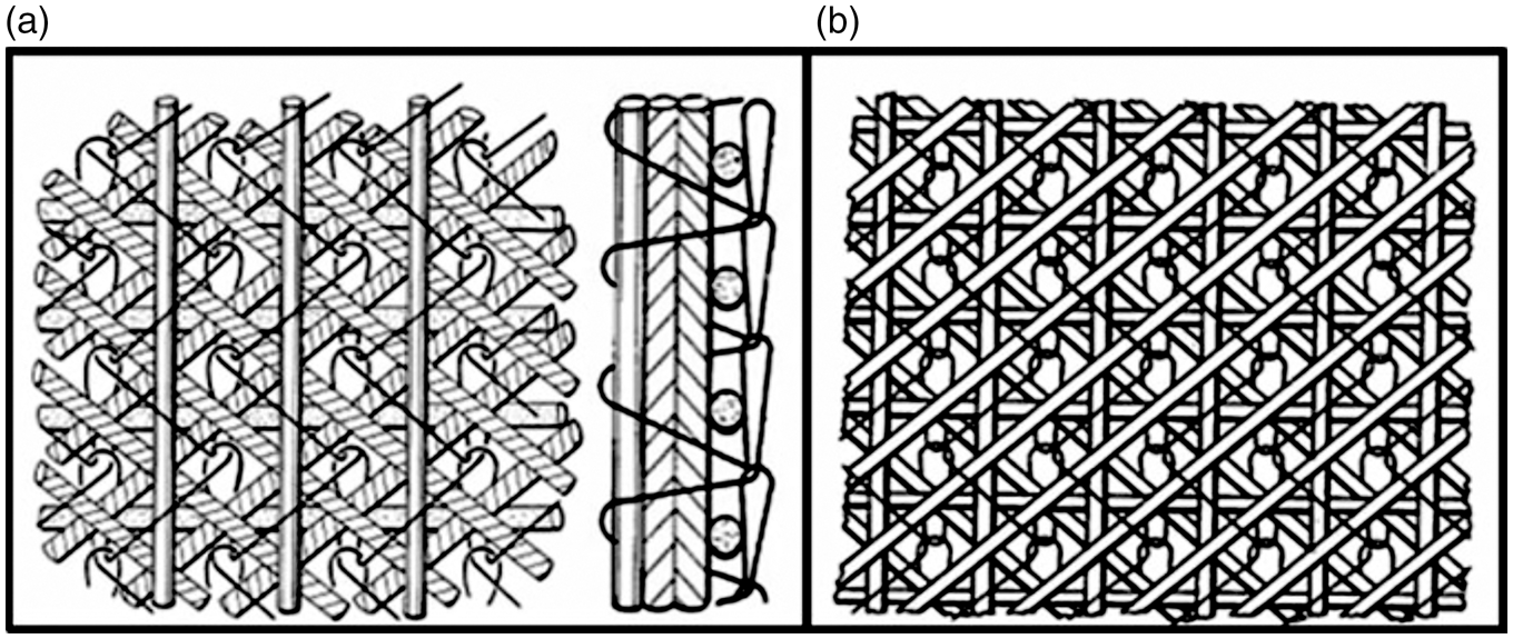

In spite of most loads being carried out by the inserted high-performance yarns in textile composite reinforcements, there are some effects of base structures and their materials on the breaking strengths of the final composites. For these effects two examples of research results can be given here as below.

Araujo et al.⁵ made two types of glass composites using fleecy weft knitted fabrics; in one of which the basic fabrics were polyester and the fleecy yarns were glass, while in the other type both the basic fabrics and the fleecy yarns were glass. Polyester/glass composites gave higher course-wise breaking strengths than glass/glass composites.

Stolyarov et al.⁶ worked on the bi-axial concrete composites by inserting glass and carbon rovings in wale-wise and glass rovings in course-wise directions of three polyester single bar warp knitted fabrics. The basic warp knitted structures were such that the first one was closed-chain stitches connected by the weft inserted glass rovings, while the second one was 1 and 1 closed-lap single bar fabric (the single Tricot) and the third one was 2 and 1 closed-lap single bar fabric (the cord). It was concluded that the Tricot fabric concrete composites gave higher wale-wise tensile strengths than the others.

The creation of geometric models of single bar warp knitted fabrics would be a basic work for obtaining the geometric models of two guide bar warp knitted fabrics as well as for obtaining geometrical models of multiaxis textile composite reinforcements. Therefore, it was decided to create proper geometrical models for the single bar warp knitted fabrics here in this work as Part II.

As explained in the general introduction in Part I,⁷ the early geometrical models^8–13 had discontinuities in their loop parts and later created models^14–16 used NURBS (Non Uniform Basis Spline) curves so that they needed some control points to obtain the models. In the present models, however, known curves will be used so that only measurable loop parameters will be used and continuities in loop parts will be attained as much as possible.

During the creation of the models, the out of fabric plane spiralities of the heads of the loops are assumed not to occur for simplicity reasons.

The creation of closed-lap single bar warp knitted fabric models will be given in the first section and then the creation of open-lap single bar warp knitted fabric models will be given in the second section.

Constructions of the closed-lap single bar warp knitted fabric models

The 1 and 1 closed-lap single bar warp knitted fabric is modeled first, and then this model is applied to the other closed-lap single bar fabrics.

Model of the 1 and 1 closed-lap single bar fabrics

Schematic drawings of the 1 and 1 closed-lap single bar warp knitted fabric are given in Figure 5.

Figure 5.

Schematic drawing of 1 and 1 closed-lap single bar warp knitted fabric loop according to the present model.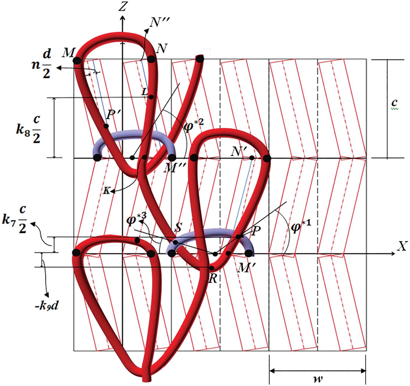

When the loop part P, R, S, K, L, N, M, $P'$ in Figure 5 is modeled, the whole structure can be obtained because of the symmetry in the structure. Modeling is done part by part as follows. Assumptions about the curves and the structure will be given during modeling of the related part.

Loop head (N, M in Figure 5)

The distance between M and N can be assumed from the situations of the loop arms given in Figures 5 and 6 as

\bar{MN} = 2 A_{uu} = \sqrt{(Z_{N} - Z_{M})^{2} + (X_{N} - X_{M})^{2}}

(1)

where

\begin{matrix} X_{N} = \frac{w}{4} - \frac{c}{2} tan γ + \frac{d}{2} cos γ \\ X_{M} = - \frac{w}{4} - \frac{c}{2} tan γ - \frac{d}{2} cos γ \\ Z_{N} = \frac{d}{2} sin γ \end{matrix}

\begin{matrix} Z_{M} = - \frac{d}{2} sin γ \\ X_{N} - X_{M} = \frac{w}{2} + d cos γ \\ Z_{N} - Z_{M} = d sin γ \end{matrix}

where c is the course-spacing, w is the wale-spacing, γ is the loop leaning angle and d is the effective yarn diameter.

Figure 6.

The loop head base line MN.

Therefore, the following equation is obtained for half of the distance, $\frac{\bar{MN}}{2} = A_{uu}$

A_{uu =} \frac{1}{2} \sqrt{(\frac{w}{2} + d cos γ)^{2} + d^{2} {sin}^{2} γ}

(2)

On the other hand, the leaning angle $η_{u}$ of the loop head can be calculated as

η_{u} = {tan}^{- 1} [\frac{A_{uu}}{(d / 2) sin γ}]

(3)

Since the loop arms in Figures 5 and 6 are making an angle γ with the fabric in the wale-wise direction, the loop head curve should have tangents at points N and M that make angles $(γ - η_{u})$ with the z direction in the x z coordinate system in Figures 6 and 7.

Figure 7.

Loop head curve.

This situation can be obtained by having a parametric ellipse with the equations

\begin{matrix} x = a_{u} (1 - k_{u} ϕ) cos ϕ \\ z = b_{u} sin ϕ \end{matrix}

(4)

The derivative $\frac{dz}{dx}$ of Equation (4) can be given by

\frac{dz}{dx} = \frac{b_{u} cos ϕ}{a_{u} [- a_{u} (1 - k_{u} ϕ) sin ϕ - k_{u} cos ϕ]}

(5)

When we put $ϕ = 0$ in Equation (5)

\frac{dz}{dx} |_{ϕ = 0} = - \frac{e_{u}}{k_{u}} = - tan [\frac{π}{2} - (γ - η_{u})]

and thus

k_{u} = e_{u} tan (γ - η_{u})

(6)

is obtained, where

e_{u} = b_{u} / a_{u}

is the eccentricity of the loop head.

The MN distance can be written using the parametric ellipse as

2 A_{uu} = \bar{MN} = a_{u} (2 - k_{u} π)

(7)

From Equations (2) and (7), the major radius of parametric ellipse a_u is obtained as

a_{u} = \frac{2 A_{uu}}{(2 - k_{u} π)}

(8)

It is assumed that e_u, the eccentricity of the loop head, is equal to one

e_{u} = 1

(9)

The minor radius of the parametric ellipse can be written as

b_{u} = e_{u} a_{u} = a_{u}

(10)

The radii of curvatures of the loop head curve at points N and M can be shown to be

ρ_{N} = \frac{a_{u} [k_{u}^{2} + e_{u}^{2}]^{3 / 2}}{e_{u}}

(11)

ρ_{M} = \frac{a_{u} [k_{u}^{2} + e_{u}^{2}]^{3 / 2}}{e_{u} (1 - k_{u} π)}

(12)

In this work, the following route is taken to equalize the radii of curvatures at points M and N between the loop head curve and the arm curves.

First of all, the loop head leaning angle $α_{1}$ into the third direction (in the fabric thickness direction) is calculated by having the angle γ equal to zero

\frac{d}{2 {cos}^{2} α_{1}} = \frac{b_{uo}^{2}}{α_{u_{0}}}

and thus

α_{1} = {tan}^{- 1} [\sqrt{\frac{2 b_{uo}^{2}}{a_{u_{o}} d} - 1}]

(13)

is obtained where

\begin{matrix} a_{u_{0}} = w / 4 + d / 2 \\ b_{u_{0}} = a_{u_{0}} \end{matrix}

This $α_{1}$ value is kept constant throughout the work.

It should be noted here that the $α_{1}$ angle is measured between the horizontal y-axis direction (through the fabric direction) and the loop head plane.

The loop arm imaginary cylinders are altered from a circular cross-section (with the radius d/2) to an elliptical one, as given in Figure 8.

Figure 8.

The imaginary cylinders to wrap the loop arms.

A parameter n is taken and the following are defined

\begin{matrix} t_{12}' = (1 + n) d \\ e_{12}' = (1 - n) d \end{matrix}

(14)

\begin{matrix} t_{11}' = (1 - n) d \\ e_{11}' = (1 + n) d \end{matrix}

(15)

The equality of radii of curvatures at points N and M are given by

ρ_{N} = \frac{a_{u} [k_{u}^{2} + e_{u}^{2}]^{3 / 2}}{e_{u}} = \frac{(t_{11}')^{2}}{2 e_{11}' {cos}^{2} α_{1}}

(16)

ρ_{M} = \frac{a_{u} [k_{u}^{2} + e_{u}^{2}]}{e_{u} (1 - k_{u} π)} = \frac{(t_{12}')^{2}}{2 e_{12}' {cos}^{2} α_{1}}

(17)

When Equations (14) and (15) are put into Equations (16) and (17), parameter n is obtained as

n = \frac{1 - \sqrt[3]{1 - k_{u} π}}{1 + \sqrt[3]{1 - k_{u} π}}

(18)

Now by changing arm cylinders from circular to elliptical cross-sectioned ones, the curvatures at points M and N could be equalized without changing the loop head curve. The final equations of the loop head curve according to the XYZ coordinate system in Figure 5 can be written as

\begin{matrix} X = a_{u} [[(1 - k_{u} ϕ) cos ϕ - k_{u} \frac{π}{2}] cos η_{u} \\ - e_{u} sin α_{1} sin ϕ sin η_{u}] - \frac{c}{2} tan γ \end{matrix}

(19)

Y = a_{u} e_{u} cos α_{1} sin ϕ

(20)

\begin{matrix} Z = a_{u} [[(1 - k_{u} ϕ) cos ϕ - k_{u} \frac{π}{2}] sin η_{u} \\ + e_{u} sin α_{1} sin ϕ cos η_{u}] + 2 c \end{matrix}

(21)

where variable angle ϕ is shown in Figure 7 and it changes from zero to π.

We will continue to model loop arms but the loop connection part is modeled first as follows.

Loop connection part (P, R, S, K and L in Figure 5)

Fabric plane model of the loop connection part

Calculations can be started with finding the X and Z coordinates of the points P, R, S, K and L in Figure 5.

The coordinates of R and K can easily be obtained from Figure 5 as

X_{R} = w - k_{17} \frac{c}{2} tan γ

(22)

Z_{R} = - k_{9} d

(23)

X_{K} = \frac{w}{4} + \frac{c}{2} tan γ - \frac{d}{2 cos γ}

(24)

Z_{K} = c

(25)

For obtaining the coordinates of point P, the intersection point of the related loop head curve and $N' M'$ straight line in Figure 5 is found first, as follows.

The coordinates of $N'$ and $M'$ are

\begin{matrix} X_{N'} = \frac{w}{4} + w + \frac{c}{2} tan γ + \frac{nd}{2 cos γ} \\ Z_{N'} = c \\ X_{M'} = w + \frac{w}{4} - \frac{c}{2} tan γ + \frac{nd}{2 cos γ} \\ Z_{M}' = 0 \end{matrix}

The equation of the straight line $N' M'$ can be written as

\frac{Z - Z_{N'}}{Z_{N'} - Z_{M'}} = \frac{X - X_{N'}}{X_{N'} - X_{M'}}

and thus as the equation

Z tan γ = X - (w + \frac{w}{4} - \frac{c}{2} tan γ + \frac{nd}{2 tan γ})

(26)

is obtained.

On the other hand, equations of loop head curve that hold the loop part PRS in Figure 5 can be given by using Equations (19) and (21)

\begin{matrix} X = a_{u} [[(1 - k_{u} ϕ) cos ϕ - \frac{k_{u} π}{2}] cos η_{u} \\ - e_{u} sin α_{1} sin ϕ sin η_{u}] - \frac{c}{2} tan γ + w \end{matrix}

(27)

\begin{matrix} Z = a_{u} [[(1 - k_{u} ϕ) cos ϕ - \frac{k_{u} π}{2}] sin η_{u} \\ + e_{u} sin α_{1} sin ϕ cos η_{u}] \end{matrix}

(28)

When Equations (27) and (28) are put into Equation (26) and defining intersection angle $ϕ^{* 1}$ , the following equation is obtained to solve for $ϕ^{* 1}$

\begin{matrix} f ϕ^{* 1} = a_{u} [[(1 - k_{u} ϕ^{* 1}) cos ϕ^{* 1} - \frac{k_{u} π}{2}] (cos η_{u} \\ - sin η_{u} tan γ) - e_{u} sin α_{1} sin ϕ^{* 1} (sin η_{u} \\ + cos η_{u} tan γ)] - (\frac{w}{4} + \frac{nd}{2 tan γ}) = 0 \end{matrix}

(29)

The intersection angle $ϕ^{* 1}$ is solved using the Newton–Raphson method and thus the following coordinates are obtained

\begin{matrix} X_{P'} = a_{u} [[(1 - k_{u} ϕ^{* 1}) cos ϕ^{* 1} - \frac{k_{u} π}{2}] cos η_{u} \\ - e_{u} sin α_{1} sin ϕ^{* 1} sin η_{u}] - \frac{c}{2} tan γ + w \end{matrix}

(30)

\begin{matrix} Z_{P'} = a_{u} [[(1 - k_{u} ϕ^{* 1}) cos ϕ^{* 1} - \frac{k_{u} π}{2}] sin η_{u} \\ + e_{u} sin α_{1} sin ϕ^{* 1} cos η_{u}] \end{matrix}

(31)

The place of L can be obtained in a similar manner with the point P as follows.

Intersection point of the $M ″ N ″$ straight line and the related loop head curve are found first as follows.

The coordinates of points $M ″$ and $N ″$ are given as

\begin{matrix} X_{N ″} = \frac{w}{4} - \frac{c}{2} tan γ - \frac{nd}{2 cos γ} \\ Z_{N ″} = 2 c \\ X_{M ″} = \frac{w}{4} + \frac{c}{2} tan γ - \frac{nd}{2 cos γ} \\ Z_{M ″} = c \end{matrix}

When the equation of the straight line is written as

\frac{Z - Z_{N ″}}{Z_{N ″} - Z_{M ″}} = \frac{X - X_{N ″}}{X_{N ″} - X_{M ″}}

and thus

Z tan γ = - X + (\frac{w}{4} + \frac{3 c}{2} tan γ - \frac{nd}{2 cos γ})

(32)

is obtained.

Again, the equations of the related loop head curve are

\begin{matrix} X = a_{u} [[(1 - k_{u} ϕ) cos ϕ - \frac{k_{u} π}{2}] cos η_{u} \\ - e_{u} sin α_{1} sin ϕ sin η_{u}] + \frac{c}{2} tan γ \end{matrix}

(33)

\begin{matrix} Z = a_{u} [[(1 - k_{u} ϕ) cos ϕ - \frac{k_{u} π}{2}] sin η_{u} \\ + e_{u} sin ϕ sin α_{1} cos η_{u}] + c \end{matrix}

(34)

The intersection point is found by putting Equations (33) and (34) into Equation (32) and thus the following equation is obtained

\begin{matrix} f ϕ^{* 2} = a_{u} [[(1 - k_{u} ϕ^{* 2}) cos ϕ^{* 2} - \frac{k_{u} π}{2}] \\ \times (cos η_{u} - sin η_{u} tan γ) - e_{u} sin α_{1} sin ϕ^{* 2} \\ \times (sin η_{u} + cos η_{u} tan γ)] + \frac{w}{4} - \frac{nd}{2 cos γ} = 0 \end{matrix}

(35)

where

ϕ^{* 2}

is the intersection angle at the loop head.

Equation (35) is solved by using the Newton–Raphson method and $ϕ^{* 2}$ is obtained. After finding $ϕ^{* 2}$ , the coordinates of point $L'$ can be written as

\begin{matrix} X_{L'} = - a_{u} [[(1 - k_{u} ϕ^{* 2}) cos ϕ^{* 2} - \frac{k_{u} π}{2}] cos η_{u} \\ - e_{u} sin α_{1} sin ϕ^{* 2} sin η_{u}] + \frac{c}{2} tan γ \end{matrix}

(36)

\begin{matrix} Z_{L'} = a_{u} [[(1 - k_{u} ϕ^{* 2}) cos ϕ^{* 2} - \frac{k_{u} π}{2}] sin η_{u} \\ + e_{u} sin α_{1} sin ϕ^{* 2} cos η_{u}] + c \end{matrix}

(37)

Estimation of the place of point, S, is not as easy as the other points, and thus this will be explained in three stages as follows.

The intersection point of the related loop head curve and the straight line (passing through) connecting points K and R is the first approximation of point S.

The coordinates of points K and R are

X_{K} = \frac{w}{4} + \frac{c}{2} tan γ - \frac{d}{2 cos γ}

(38)

Z_{K} = c

(39)

X_{R} = w - \frac{c}{2} tan γ

(40)

Z_{R} = - k_{9} d

(41)

The equation of the straight line passing through points K and R can be given by

\frac{Z - Z_{K}}{Z_{K} - Z_{R}} = \frac{X - X_{K}}{X_{K} - X_{R}}

(42)

When the values of points K and R in Equations (38)–(41) are put into Equation (42), an equation is obtained as

\begin{matrix} f ϕ^{* 3} = (Z_{S}' - c) (\frac{3 w}{4} - c tan γ + \frac{d}{2 cos γ}) \\ + (c + k_{9} d) [X_{S}' - (\frac{w}{4} + \frac{c}{2} tan γ - \frac{d}{2 cos γ})] = 0 \end{matrix}

(43)

where for obtaining the intersection point, the related loop head equations given below should be put into Equation (43)

\begin{matrix} X_{S}' = a_{u} [[(1 - k_{u} (π - ϕ^{* 3}) cos (π - ϕ^{* 3}) - k_{u} π / π 22] cos η_{u} \\ - e_{u} sin α_{1} sin (π - ϕ^{* 3}) sin η_{u}] - \frac{c}{2} tan γ + w \end{matrix}

(44)

\begin{matrix} Z_{s}' = a_{u} [[(1 - k_{u} (π - ϕ^{* 3})) cos (π - ϕ^{* 3}) - k_{u} π / π 22] sin η_{u} \\ + e_{u} sin α_{1} sin (π - ϕ^{* 3}) cos η_{u}] \end{matrix}

(45)

Equation (43) is solved for $ϕ^{* 3}$ using the Newton–Raphson method and the coordinates given in Equations (44) and (45) are obtained.

A parameter $k_{11}$ , which is smaller than 1, is defined and

ϕ_{S} = k_{11} ϕ^{* 3}

(46)

is used as the second approximation. The new coordinates of point S become

\begin{matrix} X_{S} = a_{u} [[(1 - k_{u} (π - ϕ_{S})) cos (π - ϕ_{S}) - k_{u} π / π 22] cos η_{u} \\ - e_{u} sin α_{1} sin (π - ϕ_{S}) sin η_{u}] - \frac{c}{2} tan γ + w \end{matrix}

(47)

\begin{matrix} Z_{S} = a_{u} [[1 - k_{u} (π - ϕ_{S})) cos (π - ϕ_{S}) - k_{u} π / π 22] sin η_{u} \\ + e_{u} sin α_{1} sin (π - ϕ_{S}) cos η_{u}] \end{matrix}

(48)

During modeling of the loop connection part, $k_{11}$ is controlled if Equations (47) and (48) satisfy the real loop connection part model; if not, $k_{11}$ is changed and the computer program is run again until the real loop connection part model is satisfied.

The following parameters are also defined before applying the fabric plane curve of the loop connection part

x_{L} = X_{L} - X_{K}

(49)

y_{L} = Z_{L} - Z_{K}

(50)

x_{P} = X_{P} - X_{R}

(51)

y_{P} = Z_{P} - Z_{R}

(52)

p = X_{R} - X_{K}

(53)

q = Z_{K} - Z_{R}

(54)

Using Equations (49)–(54), two connected parabolas are defined as given in Figure 9. The defined two parabolas in Figure 9 are assumed to construct the model of the loop connection part in the fabric plane.

Figure 9.

The defined two parabolas to obtain the fabric plane curve of the loop connection part.

For a given k value, parameters a₂, ϑ, a₃ and η of the parabolas in Figure 9 can be calculated. Calculations of these parameters are too lengthy to give here, and therefore they are given in Appendix A.

Equations to draw the fabric plane curve of the loop connection part in the XZ coordinate system in Figure 5 are as follows.

For part PR in Figure 5 and 9

\begin{matrix} (0 \leq u \leq u_{p}) \\ X = p + u cos ϑ - a_{2} u^{2} sin ϑ + X_{K} \end{matrix}

(55)

Z = u sin ϑ + a_{2} u^{2} cos ϑ + Z_{R}

(56)

For part RI (0 $\leq u \leq u_{I})$

X = p - u cos ϑ - a_{2} u^{2} sin ϑ + X_{K}

(57)

Z = - u cos ϑ + a_{2} u^{2} cos ϑ + Z_{R}

(58)

$Forpart IK (0 \leq \sqrt{x'} \leq \sqrt{x_{I}'}$ )

X = x' cos η + \frac{\sqrt{x'}}{\sqrt{a_{3}}} sin η + X_{K}

(59)

Z = q + x' sin η - \frac{\sqrt{x'}}{\sqrt{a_{3}}} cos η + Z_{R}

(60)

For part KL (0 $\leq \sqrt{x'} \leq \sqrt{x_{L}'})$

X = x' cos η - \frac{\sqrt{x'}}{\sqrt{a_{3}}} sin η + X_{K}

(61)

Z = q + x' sin η + \frac{\sqrt{x'}}{\sqrt{a_{3}}} cos η + Z_{R}

(62)

where the equations of the parabolas

v = a_{2} u^{2}

(63)

x' = a_{3} (y')^{2}

(64)

are used during the derivations of Equations (55)–(62).

At this point, the $k_{11}$ value of the place of point S in Figure 5 can be controlled by a control equation

\begin{matrix} f_{TU 1} = a_{2} [(Z_{S} - Z_{R}) sin ϑ + (X_{S} - p - X_{K}) cos ϑ]^{2} \\ + (X_{S} - p - X_{K}) sin ϑ - (Z_{S} - Z_{R}) cos ϑ = 0 \end{matrix}

(65)

Equalizing the tangents at points P and L, which are the points between parts of the loop, is necessary. Therefore, the $α_{P}$ and $α_{L}$ angles in Figure 9 are calculated as follows.

At point P if the differentiation $\frac{d X}{d Z} | P$ is taken as

\frac{d X}{d Z} | P = \frac{cos ϑ - 2 a_{2} u_{P} sin ϑ}{sin ϑ + 2 a_{2} u_{P} cos ϑ} = tan α_{P}

(66)

then

tan α_{P} = \frac{1 - 2 a_{2} u_{P} tan ϑ}{tan ϑ + 2 a_{2} u_{P}}

(67)

is obtained.

When the equation

2 a_{2} u_{P} = tan χ_{P}

(68)

is defined and put into Equation (66)

tan α_{P} = tan [\frac{π}{2} - (χ_{P} + ϑ)]

(69)

can be derived. Therefore

α_{P} = \frac{π}{2} - (χ_{P} + ϑ)

(70)

is found, where

χ_{P}

is as

χ_{P} = {tan}^{- 1} [2 a_{2} u_{P}]

(71)

The parameter u_P in Equation (71), in turn, can be found from Equations (55)–(62) as

u_{P} = | \frac{cos ϑ - \sqrt{{cos}^{2} ϑ - 4 a_{2} sin ϑ (X_{P} - X_{K} - p)}}{2 a_{2} sin ϑ} |

(72)

At point L, again if the differentiation $\frac{d X}{d Z} | L$ is taken as

\frac{d X}{d Z} | L = \frac{cos η - \frac{1}{2 \sqrt{x_{L}'} \sqrt{a_{3}}} sin η}{sin η + \frac{1}{2 \sqrt{x_{L}'} \sqrt{a_{3}}} cos η} = tan α_{L}

the tangent equation at L is obtained as

tan α_{L} = \frac{2 \sqrt{x_{L}'} \sqrt{a_{3}} - tan η}{1 + 2 \sqrt{x_{L}'} \sqrt{a_{3}} tan η}

(73)

When the equation below is defined

2 \sqrt{x_{L}'} \sqrt{a_{3}} = tan χ_{L}

(74)

and put into Equation (73), an equation is reached as

tan α_{L} = tan (χ_{L} - η)

(75)

From Equation (75), parameter $α_{L}$ can be found as

α_{L} = χ_{L} - η

(76)

where

χ_{L}

χ_{L} = {tan}^{- 1} [2 \sqrt{x_{L}'} \sqrt{a_{3}}]

(77)

where

\sqrt{x_{L}'}

, in turn, is obtained from Equations (55)–(62) as

\sqrt{x_{L}'} = | \frac{sin η - \sqrt{{sin}^{2} η + 4 a_{3} cos η (X_{L} - X_{K})}}{2 \sqrt{a_{3}} cos η} |

(78)

Through fabric model of the loop connection part

The loop connection part through the fabric model is given in Figure 10.

Figure 10.

The through fabric model of the loop connection part.

The Z coordinates in Figure 10 are known from Equations (55)–(62). The Y coordinates of the reference points can be given as below

Y_{P} = - k_{5} d / 2

(79)

Y_{S} = e_{a} a_{α} cos α_{1} cos ϕ_{S} + d

(80)

Y_{L} = - k_{10} d / 2

(81)

Similar curves as in the present model were given in part I⁷; therefore, they are not given here again. The only difference is that while the three-dimensional XYZ curve, between P and S, in Figure 10 was drawn by having a cylindrical object in which its axis was in the horizontal X direction in Part I,⁷ as shown in Figure 11(a), in the present work the axis of the cylindrical object is drawn in the u direction as given in Figure 11(b).

Figure 11.

Imaginary cylinders to wrap the yarn axis of the loop connection parts: (a) imaginary cylinder used for the chain stitches; (b) imaginary cylinder used in the present work.

For replacing the PRS part in Figure 11(b) from Figure 11(a), u_P and u_s are obtained as

u_{P} = | \frac{cos ϑ - \sqrt{{cos}^{2} ϑ - 4 a_{2} sin ϑ (X_{P} - X_{K} - p)}}{2 a_{2} sin ϑ} |

(82)

u_{S} = | \frac{- cos ϑ + \sqrt{{cos}^{2} ϑ + 4 a_{2} sin ϑ (p + X_{K} - X_{S})}}{2 a_{2} sin ϑ} |

(83)

For parameters v_P and v_S, the parabolic equations can be written as

v_{P} = a_{2} u_{P}^{2}

(84)

v_{s} = a_{2} u_{S}^{2}

(85)

Then u_P, v_P, u_s and v_s can be put in place of X_P, Z_P, X_S and Z_S, respectively, in the region PRS of Part I.

The same equations for the radii of curvatures in the v–Y plane at points P and S are used, which were given in Part I⁷ as Equations (35) and (36). The equations were

ρ_{P} = \frac{A_{a} e_{a}^{2}}{{cos}^{3} η (1 + k_{a} \frac{π}{2})}

(86)

ρ_{S} = \frac{A_{a} e_{a}^{2}}{{cos}^{3} η (1 - k_{a} \frac{π}{2})}

(87)

When the radii of curvatures of the cross-section of the cylindrical objects $ρ_{P}$ and $ρ_{S}$ are considered together with the helically wrapped yarn axes on these cylindrical objects, the total radii of curvatures of the yarn axes can be obtained as

ϱ_{pyarn} = \frac{ϱ_{P}}{{cos}^{2} (α_{P} + ϑ)}

(88)

ϱ_{syarn} = \frac{ϱ_{s}}{{cos}^{2} (α_{S} + ϑ)}

(89)

where

χ_{S} = {tan}^{- 1} [2 a_{2} u_{S}]

(90)

α_{S} = | \frac{π}{2} - (χ_{S} - ϑ) |

(91)

can be found using similar calculations for the ones for

α_{P}

It should be noted here that the $ρ_{pyarn}$ and $ρ_{syarn}$ radii of curvatures are the radii of curvatures of three-dimensional cylindrical object in the v–Y plane, as was the case in Part I.⁷ This situation will be considered during modeling of the loop arm curves.

Loop arms

Together with the modeling of the loop head, in the loop arm yarn axes were wrapped, the circular cross-sectioned ones were replaced by the elliptical cross-sectioned ones, as explained in Equations (14)-(18). Those changes were made to attain curvature equalities at points N and M. The curvatures at N and M were, in turn, are different from each other because of loop leaning angle γ, which occurred in the course-wise direction. The final major and minor diameters of the elliptical cross-sections were $e_{11}'$ and $t_{11}'$ for the right arm and $e_{12}'$ and $t_{12}'$ for the left arm.

However, the loop arms continue to be modeled from the state at which they are already wrapped on the elliptical cross-sectioned cylinders.

Replacing of the yarn wrapping elliptical cylinders is necessary again to obtain curvature equalities at points $P'$ and L and also without changing the curvature of the yarn arms at points M and N. The elliptical cylinders, however, can be replaced by the conical ones with satisfying the above conditions and, at the same time, obtaining variable curvatures at points $P'$ and L, as explained below.

Right arm (NL in Figure 5)

The elliptical cross-sectioned cylinder is replaced by a conical one, as given in Figure 12.

Figure 12.

Replacing elliptical cylinder with the conical one for wrapping the right arm of the loop, NL.

The Parameters of the conical object in Figure 12 can be given as

e_{11} = k_{10}^{2} e_{11}'

(92)

t_{11} = k_{10} t_{11}'

(93)

t_{2 L} = t_{11}

(94)

h_{1}' = \frac{2 c - z_{L}}{cos γ}

(95)

{AA}_{1} = \frac{2 h_{1}'}{e_{11}'}

(96)

ϑ_{K 1} = {tan}^{- 1} [\frac{- {AA}_{1} + k_{10}^{2} \sqrt{{AA}_{1}^{2} - k_{10}^{4} + 1}}{{AA}_{1}^{2} - k_{10}^{4}}]

(97)

e_{2 L} = \frac{e_{11}'}{cos ϑ_{K_{1}}}

(98)

h_{1} = (h_{1}' - \frac{e_{11}'}{2} tan ϑ_{K_{1}}) cos ϑ_{K_{1}}

(99)

The equality of the radii of curvatures at point L can be given by an equation as

\frac{ρ_{L}}{{cos}^{2} α_{L}} = \frac{e_{2 L}^{2}}{2 t_{2 L} {cos}^{2} (α_{2 L})}

(100)

where

α_{L}

was given in Equation (65) and

ρ_{L}

was calculated during obtaining the through fabric model of loop connection part, as given in Part I.⁷

The angle $α_{2 L}$ can be calculated from Figure 13

\begin{matrix} α_{2 L} + α_{L} + (γ + ϑ_{K_{1}}) = π / 2 \\ α_{2 L} = \frac{π}{2} - (α_{L} + γ + ϑ_{K_{1}}) \end{matrix}

(101)

Figure 13.

The angular analysis of the right arm of the loop at point L.

From Equation (100), the length k₁ of the cosine curve is calculated as

k_{1} = π N_{1} \sqrt{ρ_{L} A_{coseg}}

(102)

The parameters used in Equation (102) were explained in Part I⁷ during obtaining of the through fabric model of the loop connection part, and therefore they are not repeated here again.

The yarn wrapping angle on the right arm is

δ = \frac{π}{2}

(103)

Now, the yarn arm curve can be applied on the defined conical object. The cubic equation given below is suggested as the yarn arm curve

z' = a_{1}' S_{1}^{3} + b_{1}' S_{1}^{2} + c_{1}' S_{1} + d_{1}'

(104)

where

z'

is the length on the conical object, S₁ is the peripheral arc length of the conical object and

a_{1}', b_{1}', c_{1}' and d_{1}' aretheconstants .

The parameter S₁ can be found as follows.

The cross-section of the conical object is defined as

x = [\frac{e_{11}}{2} - \frac{1}{2} (e_{11} - e_{2 L}) \frac{2 ϕ}{π}] cos ϕ

(105)

y = - \frac{t_{11}}{2} sin ϕ

(106)

The derivative of Equations (105) and (106) gives

\begin{matrix} \frac{dx'}{d ϕ} = - [\frac{e_{11}}{2} - \frac{1}{2} (e_{11} - e_{2 L}) \frac{2 ϕ}{π}] sin ϕ \\ - \frac{1}{2} (e_{11} - e_{2 L}) \frac{2}{π} cos ϕ \end{matrix}

(107)

\frac{dy'}{d ϕ} = - \frac{t_{11}}{2} cos ϕ

(108)

Thus, the parameter S₁ is written as

S_{1} = \int_{ϕ = 0}^{ϕ} \sqrt{(\frac{dx'}{d ϕ})^{2} + (\frac{dy'}{d ϕ})^{2}} d ϕ

(109)

When Equation (104) is differentiated with respect to S₁, the tangent of the helix angle, α, can be obtained as

\frac{dz'}{d S_{1}} = tan α

(110)

where

\frac{dz'}{d S_{1}} = 3 a_{1}' S_{1}^{2} + 2 b_{1}' S_{1} + c_{1}'

(111)

The term tan α is also called u as follows

u = tan α

(112)

When the values of points N ( $ϕ = 0, Z' = 0, S_{1} = 0, tan α_{11} = u_{11}$ ) and L ( $ϕ = \frac{π}{2},$ $z' = h_{1}$ , $S_{1} = E_{11}$ , $tan α_{2 L} = u_{2 L}$ ) are replaced in Equations (104) and (111), the constants are obtained as given below

a_{1}' = \frac{(u_{11} + u_{2 L}) E_{11} - 2 h_{1}}{E_{11}^{3}}

(113)

b_{1}' = - \frac{(u_{2 L} + 2 u_{11}) E_{11} - 3 h_{1}}{E_{11}^{2}}

(114)

c_{1}' = u_{11}

(115)

d_{1}' = 0

(116)

$E_{11}$ in the above equations is the completion of the integral given in Equation (109)

E_{11} = \int_{ϕ = 0}^{\frac{π}{2}} \sqrt{(\frac{dx'}{d ϕ})^{2} + (\frac{dy'}{d ϕ})^{2}} d ϕ

(117)

The right arm model is completed and can be drawn now.

Left arm (M $P^{'} inFigure 5)$

The application of the conical object in place of the elliptical cross-sectioned cylindrical object for the left arm is given in Figure 14.

Figure 14.

Replacing the elliptical cylinder with the conical one for wrapping the left arm of the loop, MP′.

The parameters of the conical object can be given by

\begin{matrix} k_{5} = k_{2} < 1 \\ h_{2}' = \frac{c - Z_{P}}{cos γ} \end{matrix}

(118)

{AA}_{2} = \frac{2 h_{2}'}{e_{12}'}

(119)

ϑ_{K 2} = {tan}^{- 1} [\frac{{AA}_{2} - k_{5}^{2} \sqrt{{AA}_{2}^{2} - k_{5}^{4} + 1}}{{AA}_{2}^{2} - k_{5}^{4}}]

(120)

e_{2 P} = \frac{e_{12}'}{cos ϑ_{K 2}}

(121)

e_{12} = k_{5}^{2} e_{12}'

(122)

t_{12} = k_{5} t_{12}'

(123)

t_{2 P} = t_{12}

(124)

h_{2} = (h_{2}' + \frac{e_{12}'}{2} tan ϑ_{K 2}) cos ϑ_{K 2}

(125)

The equality of curvatures at point $P'$ is written as

\frac{ρ_{P}}{{cos}^{2} (α_{P} + ϑ)} = \frac{e_{2 P}^{2}}{2 t_{2 P} {cos}^{2} (α_{2 P})}

(126)

The angle $α_{P}$ was obtained in Equation (70). The ϑ angle is added in Equation (126), because the cylinder, on which the loop connection part is laid, is extending in the u direction instead of the X direction. $ρ_{P}$ was obtained in Part I during modeling of the through fabric model of the loop connection part. The angle $α_{2 P}$ can be written from the geometry given in Figure 15 as

α_{2 P} + α_{P} = \frac{π}{2} + (γ + ϑ_{K 2})

and thus

α_{2 P} = \frac{π}{2} + (γ + ϑ_{K 2}) - α_{P}

(127)

Figure 15.

The angular analysis of the left arm of the loop at point P′.

Equation (126) is satisfied by adjusting the parameter $k_{2} (= k_{5}); thus, k_{2} (= k_{5})$ is fixed when Equation (126) is satisfied.

The total wrapping angle, δ, of the yarn axis on the conical object is

δ = \frac{π}{2}

(128)

The yarn arm curve can now be applied on this defined conical object, suggesting a cubic polynomial

z' = a_{2}' S_{1}^{3} + b_{2}' S_{1}^{2} + c_{2}' S_{1} + d_{2}'

(129)

where

z'

is the length on the axis of the conical object.

S₁ is the peripheral arc length on the surface of the conical object, and $a_{2}'$ , $b_{2}'$ , $c_{2}'$ and $d_{2}'$ are the constants.

The parameter S₁ is defined as follows.

The cross-section of the conical object can be defined by the local coordinate system $x'$ and $y'$ as

x' = [\frac{e_{12}}{2} - \frac{1}{2} (e_{12} - e_{2 P}) \frac{2 ϕ}{π}] cos ϕ

(130)

y' = - \frac{t_{12}}{2} sin ϕ

(131)

The derivative of Equations (130) and (131) can be given by

\begin{matrix} \frac{dx'}{d ϕ} = - [\frac{e_{12}}{2} - \frac{1}{2} (e_{12} - e_{2 P}) \frac{2 ϕ}{π}] sin ϕ \\ - \frac{1}{2} (e_{12} - e_{2 P}) \frac{2}{π} cos ϕ \end{matrix}

(132)

\frac{dy'}{d ϕ} = - \frac{t_{12}}{2} cos ϕ

(133)

S₁ is then given by

S_{1} = \int_{ϕ = 0}^{ϕ} \sqrt{(\frac{dx'}{d ϕ})^{2} + (\frac{dy'}{d ϕ})} d ϕ

(134)

The derivative of $z'$ in Equation (129) with respect to S₁ gives the tangent of the helix angle α as

\frac{dz'}{d S_{1}} = tan α = 3 a_{2}' S_{1}^{2} + 2 b_{2}' S_{1} + c_{2}'

(135)

The tangent of the helix angle is also called known as u

tan α = u

(136)

When the values of points M ( $ϕ = 0, z' = 0, S_{1} = 0, tan α_{12} = u_{12}) and P' (ϕ = \frac{π}{2}, z' = h_{2}, S_{1} = E_{12}, tan α_{2 P} = u_{2 P})$ are put into Equations (129) and (135), the constants of Equation (129) are obtained as below

a_{2}' = \frac{(u_{12} + u_{2 P}) E_{12} - 2 h_{2}}{E_{12}^{3}}

(137)

b_{2}' = - \frac{(u_{2 P} + 2 u_{12}) E_{12} - 3 h_{2}}{E_{12}^{2}}

(138)

c_{2}' = u_{12}

(139)

d_{2}' = 0

(140)

The creation of the 1 and 1 closed-lap single bar warp knitted fabric model is completed now. The X, Y and Z coordinates of the drawn 1 and 1 closed-lap repeating unit of the single bar fabric model are given in Appendix B.

Models for the 2 and 1, 3 and 1, and 4 and 1 closed-lap single bar warp knitted fabrics

Similar calculations are done to obtain models of these fabrics as were carried out for the 1 and 1 closed-lap single bar warp knitted fabric. The only differences are the fabric plane models of the loop connection parts. The same calculations are also carried out for obtaining the models of the loop connection part fabric plane curves of the present fabrics, but instead of taking one wale-spacing (w) in the course direction 2w, 3w and 4w wale-spacings are taken for the 2 and 1, 3 and 1 and 4 and 1 closed-lap single bar warp knitted fabrics, respectively. The calculations given in Appendix A are used for the present fabrics.

Constructions of the open-lap single bar warp knitted fabric models

The model of the 2 and 1 open-lap single bar warp knitted fabric is created first, then the model is applied to the other open-lap single bar fabrics by changing some parts of the 2 and 1 open-lap model.

Model of the 2 and 1 open-lap single bar fabric

Schematic drawings of the 2 and 1 open-lap single bar warp knitted fabric are given in Figure 16.

Figure 16.

Schematic drawing of the repeating unit of the 2 and 1 open-lap single bar warp knitted fabric.

Because of symmetry, when the curve following points P, R, S, K, L, M, N and P’ in Figure 16 is modeled, the model of the whole the structure can be obtained. Modeling is done part by part as given in the following. It should be noted here that assumptions about the curves and the structure are given throughout the section while modeling each part.

Loop head (N, M in Figure 16)

The loop head is modeled as in the first section, and therefore it is not repeated here again.

Loop connection part (parts P, R, S, K and L in Figure 16)

Fabric plane model of the loop connection part

The fabric plane coordinates (X and Z coordinates in Figure 16) of points P, R, K, L and S in Figure 16 are defined as

X_{P} = w - \frac{w}{4} - \frac{c}{2} tan γ + k_{7} \frac{c}{2} tan γ + \frac{nd}{2 cos γ}

(141)

Z_{P} = k_{7} \frac{c}{2}

(142)

X_{R} = w - \frac{w}{4} - \frac{c}{2} tan γ + \frac{d}{2} cos γ

(143)

Z_{R} = - k_{9} d

(144)

X_{K} = - \frac{w}{4} + \frac{c}{2} tan γ + \frac{d}{2} cos γ

(145)

Z_{K} = c

(146)

X_{L} = - \frac{w}{4} + \frac{c}{2} tan γ - k_{8} \frac{c}{2} tan γ - \frac{hd}{2 cos γ}

(147)

Z_{L} = k_{8} \frac{c}{2} + c

(148)

It is not so easy to calculate the X_S and Z_S coordinates of point S, so estimation of them is given in the three steps as follows.

The first step.

A line in Figure 16 is defined as

\frac{X_{S}' - (X_{R} - \frac{d}{2} cos γ)}{(X_{R} - \frac{d}{2} cos γ) - X_{K}} = \frac{Z_{S}' - Z_{R}}{Z_{R} - Z_{K}}

and thus

f ϕ^{* 3} = Sf ϕ^{* 3} Z_{s}' + X_{s}' - (w - \frac{w}{4} - \frac{c}{2} tan γ) = 0

(149)

is obtained where

Sf ϕ^{* 3} = \frac{w - c tan γ - \frac{d}{2} cos γ}{c}

(150)

The $X_{S}'$ and $Z_{s}'$ coordinates are written in a different way by thinking of point S, at the same time, on the loop head curve. Therefore the following can be written

\begin{matrix} X_{S}' = a_{u} {[(1 - k_{u} (π - ϕ^{* 3})) cos (π - ϕ^{* 3}) - k_{u} \frac{π}{2}] cos η_{u} \\ - e_{u} sin α_{1} sin (π - ϕ^{* 3}) sin η_{u}} - \frac{c}{2} tan γ + w \end{matrix}

(151)

\begin{matrix} Z_{S}' = a_{u} {[(1 - k_{u} (π - ϕ^{* 3})) cos (π - ϕ^{* 3}) - k_{u} \frac{π}{2}] sin η_{u} \\ + e_{u} sin α_{1} sin (π - ϕ^{* 3}) cos η_{u}} \end{matrix}

(152)

When Equations (151) and (152) are used to replace $X_{S}'$ and $Z_{S}'$ of Equation (149), the parameter $ϕ^{* 3}$ can be solved by applying the Newton–Raphson method.

Parameter $k_{11}$ < 1 is defined and

ϕ_{S} = k_{11} ϕ^{* 3}

(153)

is written. New equations for point S are given as in the following

\begin{matrix} X_{S} = a_{u} {[(1 - k_{u} (π - ϕ_{s})) cos (π - ϕ_{s}) - k_{u} \frac{π}{2}] cos η_{u} \\ - e_{u} sin α_{1} sin (π - ϕ_{s}) sin η_{u}} + w - \frac{c}{2} tan γ \end{matrix}

(154)

Y_{S} = a_{u} e_{u} cos α_{1} sin (π - ϕ_{s})

(155)

\begin{matrix} Z_{S} = a_{u} {[(1 - k_{u} (π - ϕ_{s})) cos (π - ϕ_{s}) - k_{u} \frac{π}{2}] sin η_{u} \\ + e_{u} sin α_{1} sin (π - ϕ_{s}) cos η_{u}} \end{matrix}

(156)

During application of the fabric plane curve of the loop connection part, the $k_{11}$ parameter is controlled if Equations (153)–(156) also satisfy the real loop connection part fabric plane curve; if not, the $k_{11}$ parameter is changed until the real loop connection part fabric plane curve is also satisfied by Equations (153)–(156).

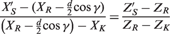
We can define the followings as well

x_{P} = X_{P} - X_{R} = - \frac{w}{4} + (1 + k_{7}) \frac{c}{2} tan γ + \frac{nd}{2 cos γ}

(157)

z_{P} = Z_{P} - Z_{R} = k_{7} \frac{c}{2} + k_{9} d

(158)

x_{L} = X_{L} - X_{K} = - k_{9} \frac{c}{2} tan γ - \frac{d}{2} cos γ - \frac{nd}{2 cos γ}

(159)

z_{L} = k_{9} \frac{c}{2}

(160)

Two more terms are also defined as given below

p = X_{R} - X_{K} = w - c tan γ

(161)

q = Z_{K} - Z_{R} = c + k_{9} d

(162)

Using the above-defined parameters, the fabric plane curve of the loop connection part is drawn in Figure 17.

Figure 17.

Modeling of the fabric plane curve of the loop connection part.

In this work it is assumed that the two parabolas given in Figure 17 construct the fabric plane model of the loop connection part.

The two parabolas intersect with each other at point I. At the same time, to be a continuous curve, the tangents of the parabolas at point I should be equalized with each other. By giving a parameter k, a₃, η, a₂ and ϑ parameters of the parabolic curves are obtained. The calculations are too lengthy to give here and therefore they are given in Appendix A.

At this point, the $k_{11}$ parameter is checked by writing

\begin{matrix} f_{TU} = a_{2} [(Z_{s} - Z_{R}) sin ϑ + (X_{s} - p - X_{K}) cos ϑ]^{2} \\ + (X_{s} - p - X_{K}) sin ϑ - (Z_{S} - Z_{R}) cos ϑ = 0 \end{matrix}

(163)

If Equation (163) is not equal to zero, $k_{11}$ is changed and the program is run again until $f_{TU}$ is equal to zero.

After obtaining a₃, η, a₂ and ϑ parameters of the parabolas, the equations of the fabric plane curve of the loop connection part are as follows.

For part PR (0 < u < u_P)

X = p + u cos ϑ - a_{2} u^{2} sin ϑ + X_{K}

(164)

Z = u sin ϑ + a_{2} u^{2} cos ϑ + Z_{R}

(165)

For part RI (0 < u < $u_{s})$

X = p - u cos ϑ - a_{2} u^{2} sin ϑ + X_{K}

(166)

Z = - u sin ϑ + a_{2} u^{2} cos ϑ + Z_{R}

(167)

For part IK (0 < $\sqrt{x'} < \sqrt{x'_{I}})$

X = x' cos η + \frac{\sqrt{x'}}{\sqrt{a_{3}}} sin η + X_{K}

(168)

Z = q + x' sin η - \frac{\sqrt{x'}}{\sqrt{a_{3}}} cos η + Z_{R}

(169)

For part KL (0 < $\sqrt{x'} < \sqrt{x'_{L}}$ )

X = x' cos η - \frac{\sqrt{x'}}{\sqrt{a_{3}}} sin η + X_{K}

(170)

Z = q + x' sin η + \frac{\sqrt{x'}}{\sqrt{a_{3}}} cos η + Z_{R}

(171)

The values of the angles $α_{P}$ and $α_{L}$ in Figure 17 are necessary for equalizing curvatures at the loop parts; therefore, their equations are given in the following.

As explained in Equations (66)–(78) in the first section, the resultant equations of angles $α_{P} and α_{L}$ can be obtained as follows

α_{P} = π / π 22 - (χ_{P} + ϑ)

(172)

where

χ_{P} = {tan}^{- 1} [2 a_{2} u_{P}]

(173)

and u_P, in turn, can be given by

u_{P} = \frac{cos ϑ - \sqrt{{cos}^{2} ϑ - 4 a_{2} sin ϑ (X_{P} - X_{K} - p)}}{2 a_{2} sin ϑ}

(174)

α_{L} = χ_{L} - η

(175)

where

χ_{L} = {tan}^{- 1} [2 \sqrt{x_{L}'} \sqrt{a_{3}}]

(176)

and

\sqrt{x_{L}'}

, in turn, can be given by

\sqrt{x_{L}'} = \frac{sin η - \sqrt{{sin}^{2} η + 4 a_{3} cos η (X_{L} - X_{K})}}{2 \sqrt{a_{3}} cos η}

(177)

It should be noted here that the $x' = a_{3} (z')^{2}$ parabolic curve did not give the curve between K and L in Figure 17; therefore, a correction equation is given as

x ″ = 0.3 + a (Z - 5)^{2}

(178)

where

a = 0.1214 (10.1481 - Z)

(179)

is calculated and (X–x′′) is taken for the curve between K and L in Figure 17.

Loop connection part through the fabric model

The Z coordinates were given in Equations (164)–(171). The Y coordinates of the reference points of the loop connection part are given as

Y_{P} = - k_{10} \frac{d}{2}

(180)

Y_{S} = e_{u} a_{u} cos α_{1} cos (π - ϕ_{s}) + d

(181)

Y_{L} = - k_{5} \frac{d}{2}

(182)

The same model for chain stitches in Part I⁷ is used here, including the extension given in the first section (see Figure 11), and therefore it is not given here again.

Loop arms

Loop arms can be modeled by wrapping the yarn axes on cylindrical objects, given in Figure 16, in which their major and the minor diameters are $e_{11}', t_{11}'$ and $e_{12}', t_{12}'$ for the right- and left-hand side arms, respectively. These cylindrical objects with elliptical cross-sections were obtained by equalizing the radii of the curvatures at points N and M in Figure 16. These objects are changed here again with the conical ones so that while the radii of the curvatures are remain the same at points N and M, changeable curvatures at points P and L in Figure 16 can be obtained. It will now be possible to equalize the radii of the curvatures at points P and L by changing the conical parameters $k_{10}$ and k₅ in Figures 18 and 19 of the conical objects, without changing the curvatures at points M and N, and thus these are explained as in the following.

Figure 18.

Application of the conical object in place of the cylindrical object for wrapping the yarn arm NP on it.

Figure 19.

For a continuous loop curve angular analysis at point P.

Right arm (NP′ in Figure 16)

In Figure 18 the major and minor diameters of the conical object are given by

e_{11} = k_{10}^{2} e_{11}'

(183)

t_{11} = k_{10} t_{11}'

(184)

e_{2 P} = \frac{e_{11}'}{cos ϑ_{K 1}}

(185)

t_{2 P} = t_{11} = k_{10} t_{11}'

(186)

where

k_{10}

is the conical parameter.

During applying of the conical object in place of the cylindrical one, the places of points N and P do not change. The curvature of the yarn axis at point N does not change with conical object application, as given in the following analysis.

The yarn radius of curvature at N was

ρ_{N} = \frac{(t_{11}')^{2}}{2 e_{11}' {cos}^{2} α_{1}}

(187)

After application of the conical object, the yarn radius of curvature at point N becomes

ρ_{N} = \frac{(k_{10} t_{11}')^{2}}{2 (k_{10}^{2} e_{11}') {cos}^{2} α_{1}} = \frac{(t_{11}')^{2}}{2 e_{11}' {cos}^{2} α_{1}}

(188)

It can be seen from Equations (187) and (188) that the yarn radius of curvature at point N does not change with the application of the conical object given in Figure 18.

On the other hand, the angle $ϑ_{K 1}$ in Equation (185) can be obtained as

h'_{1} = (c - Z_{P}) / cos γ

(189)

{AA}_{1} = \frac{2 h_{1}'}{e_{11}'}

(190)

ϑ_{K_{1}} = {tan}^{- 1} [\frac{{AA}_{1} - k_{10}^{2} \sqrt{{AA}_{1}^{2} - k_{10}^{4} + 1}}{{AA}_{1}^{2} - k_{10}^{4}}]

(191)

The length h₁ of the conical object is

h_{1} = (h_{1}' - \frac{e_{11}'}{2} tan ϑ_{K_{1}}) cos ϑ_{K 1}

(192)

The radius of curvature of the yarn axis at point P becomes

ρ_{P} = \frac{e_{2 P}^{2}}{2 t_{2 P} {cos}^{2} (α_{2 p})}

(193)

The curvature equality at point P can be satisfied by equalizing $ρ_{P_{yarn}}$ in Equation (88) and $ρ_{P}$ in Equation (193), and thus the following equation is obtained

\frac{ρ_{P}}{{cos}^{2} (α_{P} + ϑ)} = \frac{e_{2 P}^{2}}{2 t_{2 P} {cos}^{2} (α_{2 P})}

(194)

When two cylindrical objects intersect each other with helically wrapped yarn axes on them, there is a relation between the crossing angles of the cylinder axes and the total helix angles of the yarn axes at the intersection point ( $α_{P} + α_{2} + ϑ)$ to obtain continuously connected yarn axes. Let us say

α_{2 P} + (α_{P} + ϑ) = θ^{*}

(195)

The parameter $θ^{*}$ can be obtained from Figure 19 as

θ^{*} = (- α_{P} + ϑ) + α_{2 P} = \frac{π}{2} - (γ + ϑ_{K_{1}} - ϑ)

(196)

From Equations (195) and (196), $α_{2 P}$ is obtained as

α_{2 P} = \frac{π}{2} - (- α_{P} + γ + ϑ_{K_{1}})

(197)

Equation (197) can be replaced in Equation (194) and the following equation obtained

\frac{ρ_{P}}{{cos}^{2} (α_{P} + ϑ)} = \frac{e_{2 P}^{2}}{2 t_{2 P} {cos}^{2} [\frac{π}{2} - (- α_{P} + γ + ϑ_{K_{1}}]}

(198)

Equation (198) can be solved by only altering the $k_{10}$ parameter. Therefore, Equation (198) is solved by an iteration method, for example using the Newton–Raphson method, and the $k_{10}$ parameter is obtained. After finding a $k_{10}$ value to satisfy Equation (198), the other parameters can be obtained from Equations (183)–(197).

Since the conical object is fully defined by its parameters $e_{11}$ , $t_{11}$ ; $e_{2 P}$ , $t_{2 P}$ , h₁ and the yarn axis parameters on the conical object $α_{11} = α_{1}$ ; $α_{2 P}$ ; $δ = π / 2$ (total yarn wrapping angle) are known, the yarn path on the conical object can be assumed by the following cubic equations

z' = a_{1}' S_{1}^{3} + b_{1}' S_{1}^{2} + c_{1}' S_{1} + d'

(199)

where

z'

is the cylinder length, S₁ is the peripheral length on the cross-section of the cylinder and

a_{1}'

b_{1}'

c_{1}'

and

d_{1}'

are the constants.

When a variable angle ϕ is defined on the conical object starting from the $x'$ -axis in Figure 18, S₁ can be written as follows

x' = [\frac{e_{11}}{2} - \frac{1}{2} (e_{11} - e_{2 P}) \frac{2 ϕ}{π}] cos ϕ

(200)

y' = - \frac{t_{11}}{2} sin ϕ

(201)

\begin{matrix} \frac{dx'}{d ϕ} = - [\frac{e_{11}}{2} - \frac{1}{2} (e_{11} - e_{2 P}) \frac{2 ϕ}{π}] sin ϕ \\ - \frac{1}{2} (e_{11} - e_{2 P}) \frac{2}{π} cos ϕ \end{matrix}

(202)

\frac{dy'}{d ϕ} = - \frac{t_{11}}{2} cos ϕ

(203)

{dS}_{1} = \sqrt{(\frac{dx'}{d ϕ})^{2} + (\frac{dy'}{d ϕ})^{2}} d ϕ

(204)

S_{1} = \int_{ϕ = 0}^{ϕ} \sqrt{(\frac{dx'}{d ϕ})^{2} + (\frac{dy'}{d ϕ})^{2}} d ϕ

(205)

When Equation (199) is differentiated, the following equation is obtained

\frac{dz'}{d S_{1}} = 3 a_{1}' S_{1}^{2} + 2 b_{1}' S_{1} + c_{1}' = tan α

(206)

tan α

can also be defined as in the following as well

tan α = u

(207)

When the parameters of points N and P, such as N ( $ϕ = 0$ ; $S_{1} = 0$ ; $z' = 0$ , $tan α_{11} = u_{11}$ ) and P ( $ϕ = π / 2$ ; $S_{1} = E_{11}; z' = h_{1}$ ; $tan α_{2 P} = u_{2 P}$ ), are put into Equations (199) and (206), the following equations are obtained for unknown parameters

a_{1}' = \frac{(u_{11} + u_{2 P}) E_{11} - 2 h_{1}}{E_{11}^{3}}

(208)

b_{1}' = - \frac{(u_{2 P} + 2 u_{11}) E_{11} - 3 h_{1}}{E_{11}^{2}}

(209)

c_{1}' = u_{11}

(210)

d_{1}' = 0

(211)

where

E_{11} = \int_{ϕ = 0}^{π / 2} \sqrt{(\frac{dx'}{d ϕ})^{2} + (\frac{dy'}{d ϕ})^{2}} d ϕ

(212)

Finally, the equation of the loop arm curve can be given by

x' = [\frac{e_{11}}{2} - \frac{1}{2} (e_{11} - e_{2 P}) \frac{2 ϕ}{π}] cos ϕ

(213)

y' = - \frac{t_{11}}{2} sin ϕ

(214)

z' = a_{1}' S_{1}^{3} + b_{1}' S_{1}^{2} + c_{1}' S_{1} + d_{1}'

(215)

in the local coordinate system

x' y' z'

in Figure 18.

Left arm (ML in Figure 16)

The left arm is modeled as given in Figure 20.

Figure 20.

Application of the conical object in place of the cylindrical object for wrapping the yarn arm ML on it.

Similar to the right arm model, the left arm cylinder is also replaced by a conical object, but this time conical parameter k₅ is taken, which is smaller than 1 ( $k_{5} < 1)$ . Again, the places of the points M and L are not changed and the curvature at point M is not changed by applying conical object. Very similar calculations are done to the ones that were given for the right arm, and therefore only the resultant equations are outlined in the following

h_{2}' = \frac{2 c - Z_{L}}{cos γ}

(216)

{AA}_{2} = \frac{2 h_{2}'}{e_{12}'}

(217)

ϑ_{K 2} = {tan}^{- 1} [\frac{{AA}_{2} - k_{5}^{2} \sqrt{{AA}_{2}^{2} - k_{5}^{4} + 1}}{{AA}_{2}^{2} - k_{5}^{4}}]

(218)

e_{2 L} = \frac{e_{12}'}{cos ϑ_{K 2}}

(219)

t_{2 L} = k_{5} t_{12}'

(220)

t_{12} = t_{2 L}

(221)

e_{12} = k_{5}^{2} e_{12}'

(222)

\frac{ρ_{L}}{{cos}^{2} (α_{L})} = \frac{e_{2 L}^{2}}{2 t_{2 L} {cos}^{2} (α_{2 L})}

(223)

where

α_{2 L}

is obtained from Figure 21 as

α_{2 L} = \frac{π}{2} + ϑ_{K 2} + γ - α_{L}

(224)

h_{2} = (h_{2}' + \frac{e_{12}'}{2} tan ϑ_{K 2}) cos ϑ_{K 2}

(225)

Figure 21.

For a continuous loop curve, angular analysis at point L.

Equations of the curve between M and L in Figures 20 and 21 can be given in the local coordinate system x′ y′ z′ as

x' = [\frac{e_{12}}{2} - \frac{1}{2} (e_{12} - e_{2 L}) \frac{2 ϕ}{π}] cos ϕ

(226)

y' = - \frac{t_{12}}{2} sin ϕ

(227)

z' = a_{2}' S_{1}^{3} + b_{2}' S_{1}^{2} + c_{2}' S_{1} + d_{2}'

(228)

where S₁ is the peripheral length of the cross-section of the conical object,

z'

is the cylinder length and

a_{2}', b_{2}', c_{2}'

and

d_{2}'

are constants.

Parameter S₁ is found in the following

\begin{matrix} \frac{dx'}{d ϕ} = - [\frac{e_{12}}{2} - \frac{1}{2} (e_{12} - e_{2 L}) \frac{2 ϕ}{π}] sin ϕ \\ - \frac{1}{2} (e_{12} - e_{2 L}) \frac{2}{π} cos ϕ \end{matrix}

(229)

\frac{dy'}{d ϕ} = - \frac{t_{12}}{2} cos ϕ

(230)

S_{1} = \int_{ϕ = 0}^{ϕ} \sqrt{(\frac{dx'}{d ϕ})^{2} + (\frac{dy'}{d ϕ})^{2}} d ϕ

(231)

It should be noted here that if the upper limit of ϕ is equal to $π / π 22, S_{1}$ in Equation (231) is called as $E_{12}$ , that is

E_{12} = \int_{ϕ = 0}^{π / π 22} \sqrt{(\frac{dx'}{d ϕ})^{2} + (\frac{dy'}{d ϕ})^{2}} d ϕ

(232)

The constants $a_{2}', b_{2}', c_{2}'$ and $d_{2}'$ are obtained as in the following.

When the cubic equation (228) is differentiated the following equation is obtained

\frac{dz'}{d S_{1}} = 3 a_{2}' S_{1}^{2} + 2 b_{2}' S_{1} + c_{2}' = tan α

(233)

where

tan α = u

(234)

can be written.

When the values of M and L are put into Equations (228) and (233), that is, $M (ϕ = 0; S_{1} = 0; z' = 0; tan α_{12} = u_{12})$ and $L (ϕ = π / π 22; S_{1} = E_{12}; z' = h_{2}; tan α_{2 L} = u_{2 L})$ , the following equations are obtained for constants

a_{2}' = \frac{(u_{12} + u_{2 L}) E_{12} - 2 h_{2}}{E_{12}^{3}}

(235)

b_{2}' = - \frac{(u_{2 L} + 2 u_{12}) E_{12} - 3 h_{2}}{E_{12}^{2}}

(236)

c_{2}' = u_{12}

(237)

d_{2}' = 0

(238)

A computer program is written to calculate the model and obtained the X, Y and Z coordinates of it are given as in Appendix C.

Models of the 1 and 1 and 3 and 1 open-lap single bar fabrics

The models of 1 and 1 and 3 and 1 open-lap single bar fabrics are obtained, changing the fabric plane curve of the loop connection part of the 2 and 1 open-lap single bar fabric model, as explained below.

The equation

x_{i}^{″} = w {sin}^{2} (\frac{π z_{i}^{'}}{2 z_{0}^{'}})

(239)

is defined, where w is the wale-spacing, $z_{0}^{'}$ is the difference between the starting point Z₁₀ and the last point Z₄ of the loop connection part (see Appendix C)

z_{0}' = Z_{10} - Z_{4}

(240)

and

z_{i}'

is the difference between the starting point

Z_{10}

and the point Z_i

z_{i}' = Z_{10} - Z_{i}; i = 4, \dots ., 10

(241)

For obtaining the 1 and 1 open-lap single bar fabric model, the difference ( $X_{i} - x_{i} ″$ ); i = 4,…, 10 is calculated and replaced by X_i for the loop connection part. To obtain a continuous loop shape

x_{i} = - w; i = 1, . ., 4

(242)

should also be added to the X_i coordinates.

For obtaining the 3 and 1 open-lap single bar fabric model, the term ( $X_{i} + x_{i} ″$ ); i = 4,…, 10 is calculated and replaced by X_i for the loop connection part. Again to obtain a continuous loop shape

x_{i} = w; i = 1, \dots, 4

(243)

should also be added to the X_i coordinates.

The Y and Z coordinates of the 2 and 1 open-lap single bar fabric model remain the same for the 1 and 1 open-lap and 3 and 1 open-lap single bar fabric models.

In these models, the inclination angle of loop γ is kept constant and γ = 11° is assumed to occur.

Resultant drawings of the models

The models are drawn to scale by using the 3DS-MAX computer graphical program, taking $w = 4 d$ wale–spacing and $c = 5 d$ course-spacing values, where d is the yarn diameter. The models drawn are given in Figures 22 –25 for the closed-lap and in Figures 26 –28 for the open-lap single bar warp knitted fabrics.

Figure 22.

Present model of the 1 and 1 closed-lap single bar warp knitted fabric (single Tricot), drawn to scale by using the 3DS-Max computer program.

Figure 23.

The present model of the 2 and 1 closed-lap single bar warp knitted fabric, drawn to scale by using the 3DS-Max computer program.

Figure 24.

The present model of the 3 and 1 closed-lap single bar warp knitted fabric, drawn to scale by using the 3DS-Max computer program.

Figure 25.

The present model of the 4 and 1 closed-lap single bar warp knitted fabric, drawn to scale by using the 3DS-Max computer program.

Figure 26.

Present model of the 1 and 1 open-lap single bar warp knitted fabric, drawn to scale by using the 3DS-Max computer program.

When Figures 22 –25 are examined, it is seen that while the loop connection parts of the 1 and 1 and 2 and 1 closed-lap single bar warp knitted fabrics are suitable and can be observed on real fabrics, the loop connection parts of the other fabrics, namely 3 and 1 and 4 and 1 closed-lap single bar warp knitted fabrics, should be tighter than the obtained ones. This can be overcome by having the 1 and 1 closed-lap single bar fabric model and applying very similar procedures as given by Equations (239)–(243) (for the open-lap) in place of the present loop connection parts (which are constructed by having two connected parabolas) to obtain the corrected models of the 3 and 1 and 4 and 1 closed-lap single bar warp knitted fabrics.

The 1 and 1 open-lap single bar warp knitted fabric model given in Figure 27 is obtained by using Equations (239)–(243). There are some discrepancies in the loop connection parts of this model. These discrepancies can be overcome by having a value that is smaller than w in Equation (239). In this condition, the opinion is that the touching of adjacent wales does not occur for the 1 and 1 open-lap single bar fabrics.

Figure 27.

Present model of the 2 and 1 open-lap single bar warp knitted fabric, drawn to scale by using the 3DS-Max computer program.

Figure 28.

Present model of the 3 and 1 open-lap single bar warp knitted fabric, drawn to scale by using the 3DS-Max computer program.

The models given here are general loop shapes obtained by using known curves and by satisfying the curvature equalities between the loop parts as much as possible. The models are versatile and, for obtaining special cases of them, the parts of the models can be changed easily. The methods of changing the loop shapes are given throughout the work, including the appendices.

Conclusion

Warp knitted fabrics are attractive to use for technical textile applications nowadays. This series of papers is aimed at creating models of basic warp knitted fabrics. In this context, models for the 1 and 1, 2 and 1, 3 and 1, 4 and 1 closed-lap and for the 1 and 1, 2 and 1 and 3 and 1 open-lap single bar warp knitted fabrics are created in the present work as Part II.

During modeling, loop leanings toward the course direction are considered, curvature equalities at the loop parts are attained as much as possible and two connected parabolas are used as the models for the fabric plane curves of the loop connection parts. The loop heads are taken as two-dimensional parametric ellipses. The remaining curves used are parabolic or cubic equations applied on imaginary cylindrical or conical objects.

The models given here are general loop shapes obtained by using known curves. The models are versatile and, for obtaining special cases of them, the parts of the models can be changed easily. The methods of changing the loop shapes are given throughout the work, including the appendices.

The models are drawn to scale using the 3DS-MAX computer graphical program. At first glance, it is seen that the shapes obtained from the models are similar to those observed on the real fabric samples.

Footnotes

Acknowledgements

The author would like to thank Assoc. Prof. Dr Tuba Alpyıldız and BSc students Hüseyin Hakan Güzel, Serhat Doğan, Evren Sergin, Seren Sergin and Gülsüm Kelebek for their contributions during the initial drawings of the models. The author would like to thank also Architect Darioush Bashiri, PhD student Berrak Buket Avcı, PhD student Mehmet Korkmaz, MSc student Gökberg Devrim and BSc students Mehmet Aslan and Andaç Seyrek for their contributions during the preparation of this paper.

Declaration of conflicting interests

The author declared no potential conflicts of interest with respect to the research, authorship and/or publication of this article.

Funding

The author received no financial support for the research, authorship and/or publication of this article.

References

Paling

. Warp knitting technology, Nottingham, UK: Columbine Press Ltd, 1965.

Ray

. Fundamentals and advances in knitting technology, New Delhi: Woodhead Publishing, India Pvt. Ltd, 2012.

Bilisik

Karaduman

Bilisik

Fibre architectures for composite applications. In: Fangueiro

Rana

(eds). Fibrous and textile materials for composite applications, Singapore: Springer Science + Business Media, 2016, pp. 75–134.

Bilisik

Cartesian 3D braiding. In: Kyosev

(ed). Advances in braiding technology: Specialized techniques and applications, New York: Elsevier Limited-Woodhead Publishing, 2016, pp. 107–145.

Araujo

MDe

Fangueiro

Hong

. Modelling and simulation of the mechanical behaviour of weft-knitted fabrics for technical applications Part I: general considerations and experimental analyses. AUTEX Res J 2003; 3: 112–123.

Stolyarov

Quadflieg

Gries

. Effect of fabric structures on the tensile properties of warp-knitted fabrics used as concrete reinforcements. Text Res J 2015; 85: 193–1945.

Kurbak

. Models for basic warp knitted fabrics Part I: chain stitches and their applications on marquisette, and weft inserted warp knitted fabrics. Text Res J. 2019; 89: 1863–1885.

Allison

. Warp-knitting calculations made easy. Skinner’s Silk Rayon Rec 1958; 32: 281–283.

Grosberg

. The geometry of warp-knitted fabrics. J Text Inst 1960; 51: T39–T48.

10.

Grosberg

. The geometrical properties of simple warp-knit fabrics. J Text Inst 1964; 55: T18–T30.

11.

Shinn

El-Araf

. The geometry of warp-knit structures. Knit Outerw Times 1966; 35: 24–27.

12.

Raz

. Warp knitting production, Heidelberg: Verlag Melliand Textilberichte GmbH, 1987.

13.

Hart

De Jong

Postle

. Analysis of the single-bar warp knitted fabrics using energy minimization techniques Part II: results and comparison with woven and weft knitted analysis. Text Res J 1985; 55: 530–539.

14.

Göktepe

Harlock

. Three-dimensional computer modelling of warp knitted structures. Text Res J 2002; 72: 266–272.

15.

Honglian

Mingqiao

Gaoming

. Three-dimensional computer simulation of warp knitted fabric. Fibres Text East Eur 2009; 17: 74–74.

16.

Renkens

Kyosev

. Geometry modelling of warp knitted fabrics with 3D form. Text Res J 2010; 81: 437–443.

Models for basic warp knitted fabrics Part II: single guide bar fabrics (closed-lap and open-lap)

Abstract

Keywords

Constructions of the closed-lap single bar warp knitted fabric models

Model of the 1 and 1 closed-lap single bar fabrics

Loop head (N, M in Figure 5)

Loop connection part (P, R, S, K and L in Figure 5)

Fabric plane model of the loop connection part

Through fabric model of the loop connection part

Loop arms

Right arm (NL in Figure 5)

Left arm (M P ' inFigure 5 )

Models for the 2 and 1, 3 and 1, and 4 and 1 closed-lap single bar warp knitted fabrics

Constructions of the open-lap single bar warp knitted fabric models

Model of the 2 and 1 open-lap single bar fabric

Loop head (N, M in Figure 16)

Loop connection part (parts P, R, S, K and L in Figure 16)

Fabric plane model of the loop connection part

Loop connection part through the fabric model

Loop arms

Right arm (NP′ in Figure 16)

Left arm (ML in Figure 16)

Models of the 1 and 1 and 3 and 1 open-lap single bar fabrics

Resultant drawings of the models

Conclusion

Footnotes

Acknowledgements

Declaration of conflicting interests

Funding

References

Left arm (M $P^{'} inFigure 5)$