Balancing apparel assembly lines through adaptive ant colony optimization

Abstract

The goal of this study was to introduce an effective optimization method to balancing one-piece flow assembly lines by rearranging manufacturing tasks necessary for an apparel production to minimize the number of workstations and the idle time of the assembly line under certain conditions. In this paper, we firstly define an assembly-line-balancing (ALB) problem in apparel production and established an objective function for minimizing the smoothness index, a term that measures the difference between the worktime and the targeted cycle time of each workstation on an assembly line. We then illustrate an adaptive ant colony (AAC) algorithm with modifications made on the traditional ant colony algorithm for solving the ALB problem. Finally, we present the experiments using real-world data provided by an apparel manufacturer to compare the results generated from the AAC and the prior practice of the company. It was demonstrated that the AAC could help the company reduce the number of workstations on its assembly lines and cut the idle time at most of the workstations.

Keywords

ant colony optimization one-piece flow apparel assembly line

In apparel production, an assembly line normally consists of a number of workstations, each performing specific tasks in a restrictive order.^1,2 Typically, an apparel product is assembled in a batch operation, in which multi-parts are processed in one “lot” or “group” together before being moved to the next task.³ The efficiency of the assembly line can be improved by making it more suitable for “little variety and large batch” production through a proper division of the line. However, this batch production approach is likely to bring with it batch quality problems and a high rework rate.⁴ In the era of apparel mass-customization, batch production is barely able to satisfy the demand for “multi-variety, small-batch and fast-delivery” products.

Industrial engineering (IE) technology has been adopted to assemble workstations in an orderly flow and to remove backlogs for more customizable products. Incorporating IE principles into a batch production leads to a process called one-piece flow,⁵ which means processing one item at a time and moving it through continuous processing tasks with minimal delay or waiting time.^6,7 The one-piece flow production can reduce product preparation time and manufacturing failure rate, and increase flexibility and outputs.^8,9

Usually, one workstation in the one-piece flow production contains several tasks. To make the production fluent, tasks need to be analyzed carefully, workstations must be available for the assigned tasks, and operators must be given sufficient time to perform certain tasks. The synchronization of the one-piece flow production means balancing the tasks on an assembly line to allow operators to run machines in the most efficient way¹⁰; this is the most crucial work undertaken by production planning.¹¹ An assembly-line-balancing (ALB) problem belongs to a nondeterministic polynomial optimization problem in which the number of workstations for a given cycle time and the idle time of each workstation should be minimized.¹²

The methods used to solve ALB problems can be divided into two major groups. One features optimization techniques, including the branch and bound algorithm,^13–15 dynamic programming,^16,17 linear programming,¹⁸ and integer programming.¹⁹ These optimization techniques can result in an optimal solution for small-size ALB problems, but appear to be inefficient or invalid for large-scale ALB problems. The second group is characterized by meta-heuristic techniques such as Tabu search,²⁰ genetic algorithm,^21–22 simulated annealing algorithm,²³ and the ant colony (AC) algorithm,^24–25 etc. Meta-heuristic algorithms can attain feasible solutions more efficiently both for small-size and large-size ALB problems. A performance comparison among Tabu search, genetic algorithm, simulated annealing algorithm and the AC algorithm²⁶ is given in Table 1.

Table 1.

Performance comparison of four meta-heuristic algorithms

Meta-heuristic algorithms	Advantages	Disadvantages
Tabu search	Provides a large search range	Dependent on the initial solution and difficult to select the Tabu length
Genetic algorithm	Handles constraints well and has a strong global search ability	Local search ability is weak, running time is long, and is easily affected by parameters
Simulated annealing algorithm	Simple description, strong local search ability and fewer limitations of initial conditions	Global search ability is weak, so it takes a long time to achieve the optimal solution
AC algorithm	Has a positive feedback mechanism, strong robustness and ability to search for better solutions	For large-scale problems, the search time is lengthy and may converge with the local optimal solution

Alhamdy et al.²⁷ solved a problem associated with traveling salesmen using the AC algorithm in comparison with Tabu search, simulated annealing, and the genetic algorithm. The results showed that the AC algorithm was most efficient among these compared algorithms.

AC algorithms became a popular option for solving combinatorial optimization problems. The idea of an AC algorithm comes from the foraging behavior of a real ant colony. While ants are looking for food, they always release a substance called pheromone to help the others to follow. There are many paths between a colony and a food source. Ants are able to find the shortest path after many ants have passed. This behavioral mechanism is a metaphor to describe the search process in an AC algorithm. Balancing an apparel assembly line is similar to the ant foraging behavior that finds the shortest path to the food source. Initially, a basic AC algorithm was developed for ALB.²⁸ Later, the AC algorithm was modified or combined with other methods for more specific ALB problems. For instance, Bautista and Pereira^29,30 applied AC to optimize a bike assembly line. Sabuncuoglu et al.³¹ proposed AC to solve the single-model U-type ALB problem. Baykasoglu and Dereli³² proposed an AC algorithm to solve straight-line and U-shaped ALB problems with the aim of minimizing the number of workstations. Yagmahan³³ developed a multi-objective AC algorithm to deal with the mixed ALB model to minimize the number of workstations for a given cycle time. Zha and Yu³⁴ presented a hybrid algorithm of AC and a beam search for balancing and rebalancing an assembly line in a just-in-time production environment. Kalayci and Kalayci³⁵ used an AC algorithm to balance a bathrobe production line. Zhong and Ai³⁶ modified the AC algorithm to balance a multi-objective assembly line for minimizing workstations and workload variations. However, these AC-based algorithms exhibited some weaknesses in various applications, such as a likelihood to be trapped in local minima, missing a global optimal solution, and not having been effectively applied to balancing apparel assembly lines.

In this research, we intended to develop an adaptive ant colony (AAC) algorithm to improve its ability to search for a global solution with fast convergence, and to apply it to solving the apparel ALB problems in one-piece flow productions. The main idea behind the AAC algorithm is that the global pheromone trail should be adjusted adaptively to prevent the algorithm from falling into a local optimum, by utilizing not only the external information but also the historical information of “ants.” In this paper, we will define the ALB problem, establish the mathematical model, explain the AAC algorithm for balancing the one-piece flow of an apparel assembly line, and present the experiments on real-world production data to validate the AAC algorithm.

Definition of the ALB problem

An apparel assembly line usually contains many tasks, each taking a certain time to be accomplished. One or multiple tasks can be allocated to a workstation, and thus an assembly line is made up of several orderly workstations.³⁷ An index, called the smoothness index (SI), is used to measure the effectiveness of balancing tasks on an assembly line.^38–41 One type of ALB problem, denoted as ALB-SI, is to minimize the SI when the number of workstations, the cycle time, or both are given. Solving ALB-SI is particularly useful for apparel production because allocating tasks to workstations properly to smoothen workloads in the one-piece flow is the main concern to many companies.

Many previous ALB solutions did not limit the number of machines or tools at each workstation.⁴² In apparel production, however, if operators are required to use several machines in one workstation, they have to move between the machines, making it difficult to handle different tasks within a time constraint. Thus, the machine constraint (up to two machines) will be enforced in this paper. The assumptions associated with the problem definition are listed as follows:

Time for performing each task is known.

Precedence relationships between tasks are known.

Only after the immediate predecessor task is done, one task can be operated.

Machines types are known.

Every workstation can use one or two machine types.

Total task time in each workstation cannot exceed the cycle time. The definition of cycle time is the theoretical total amount of elapsed time that a workstation spends.

The operating coefficient level of an operator is known. The coefficient level consists of four aspects: skill, effort, operating condition and consistency.

Each task must be assigned to only one workstation.

The notations and definitions of the variables used in the mathematical model are given in Table 2.

Table 2.

Notations and definitions of variables

Notation	Definition
i, j	Task number, i, j = 1, 2, … , N
N	Total number of tasks
k	Workstation number, k = 1, 2, … , K
K	Number of workstations
SI	Smoothness index
t_i	Process time of task i
C	Theoretical cycle time
X_ik	= 1 if task i is assigned to workstation k = 0 otherwise
m	Index of machine type, m = 1, 2, … , M
M	Types of machines
M_mk	= 1 if machine m is used in workstation k = 0 otherwise
Pred	Pred = {(i, j) \| task i is the predecessor task of task j}

This paper focuses on an ALB-SI in which the cycle time is given. The objective function that minimizes the SI of the assembly line is formulated as Equation 1, and the constraints of the ALB-SI are given in equations 2–8.

f (k) = SI = \sqrt{\sum_{k = 1}^{K} (\sum_{i = 1}^{N} X_{ik} \cdot t_{i} - C)^{2} / K}

(1)

where

\sum_{k = 1}^{K} X_{ik} = 1 (i = 1, 2, \dots, N)

(2)

\begin{matrix} X_{ik} = {\begin{matrix} 1 & iftask i isassignedtoworkstation k \\ 0 & otherwise \end{matrix} \end{matrix}

(3)

\sum_{k = 1}^{K} ({kX}_{jk} - {kX}_{ik}) \geq 0 ((i, j) \in Pred)

(4)

\sum_{i = 1}^{N} X_{ik} \cdot t_{i} \leq C (k = 1, 2, \dots, K)

(5)

\sum_{m = 1}^{M} M_{mk} \leq 2 (k = 1, 2, \dots, K)

(6)

M_{mk} = {\begin{matrix} 1 & if machine m is used in workstation k \\ 0 & otherwise \end{matrix}

(7)

Pred (i, j) = {\begin{matrix} 1 & if task i is the immediate predecessor \\ task of task j \\ 0 & otherwise \end{matrix}

(8)

In Equation 1, the objective function is equal to SI, which was defined based on the average difference between the total time of all the tasks in each workstation and the cycle time. Constraints (2) and (3) ensure each task is assigned to only one workstation. Constraint (4) sets the precedence requirements to ensure task i is prior to task j. Constraint (5) enforces the cycle time on all workstations, which means that the total time at all workstations cannot exceed the cycle time C. Constraints (6) and (7) ensure that there are no more than two machines at one workstation. Constraint (8) represents the precedence relationships.

An AC Algorithm

Calculation of feasible solutions

Available task set

An available task set can be created according to the precedence relationships (Equation 8). Only the tasks whose immediate antecedent tasks have been finished can be put into the available task set. According to Equation 8, Pred(i, j) = 1 when task i is the immediate predecessor of task j. Otherwise, Pred(i, j) = 0. Thus, an N × N priority matrix can be set. When task i has been chosen, it is put into a Tabu set, which saves the finished tasks.

Heuristic information

Heuristic information is critical to the AC algorithm, as it directs an ant to find a feasible path (solution). Position weights can be used to construct the heuristic information η_i:

η_{i} = \frac{{pw}_{i}}{\sum_{i = 1}^{N} {pw}_{i}}

(9)

{pw}_{i} = t_{i} + \sum_{j \in F_{i}} t_{j}

(10)

where η_i represents the expected value (the visibility) of task I; pw_i is the position weight of task I; t_i is the task time of task I; t_j is the task time of task j; and F_i is the successor task set of task i.

Task probability

The probability of a task to be chosen from an available task set is related to its heuristic information and its pheromone, which has been deposited in previous solutions. The pseudorandom proportional method is used to select a task as follows:

\begin{matrix} task i \Rightarrow {\begin{matrix} {\arg {max [τ_{ij} (t)]}_{i \in {allowed}_{j}}}^{α} [η_{i}]^{β} & 0 \leq q \leq q_{1} ① \\ p_{ij} = \frac{[τ_{ij} (t)]^{α} [η_{i}]^{β}}{\sum_{z \in {allowed}_{j}} [τ_{zj} (t)]^{α} [η_{z}]^{β}} & q_{1} < q < q_{2} ② \\ randomselection, i \in {allowed}_{j} q_{2} \leq q \leq 1 ③ \end{matrix} \end{matrix}

(11)

where τ_ij is the pheromone between task i and workstation j. The greater τ_ij, the more former “ants” that have chosen to allocate work i to workstation j. allowed_j is an available task set; α is the parameter of pheromone (α > 0); β is the parameter of heuristic information (β > 0); p_ij represents the transition probability; q is a random number in [0,1] generated by an ant when it chooses task i at workstation j; and q₁ and q₂ are tunable parameters (0 ≤ q₁ < q₂ ≤ 1). Equation 11 provides three ways to select the task that belongs to the available task set.

If 0 ≤ q ≤ q₁, the ant determines the best task according to Equation 11-① with a probability of q₁.

If q₁ < q < q₂, the ant determines the best task according to Equation 11-② with a probability of q₂ − q₁.

If q₂ ≤ q ≤ 1, the ant determines the best task according to Equation 11-③ with a probability of 1−q₂.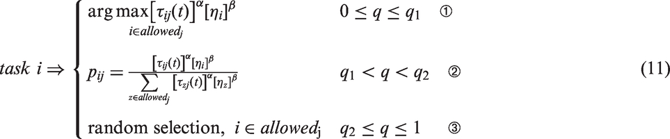

Pheromone update

There are two kinds of pheromones that need to be updated during the AAC: local and global pheromones. During the construction of a solution, after the ant assigns task i to workstation j, the local pheromone between task i and workstation j is updated by the following rule:

τ_{ij} (t) = (1 - ρ_{1}) τ_{ij} (t - 1) + ρ_{1} τ_{0}

(12)

where ρ₁ (ρ₁ ∈ [0,1]) is the local pheromone evaporation parameter, and τ₀ is the initial value of the pheromone.

The global pheromone is increased with the tasks of the best allocation, and decreased with the tasks that are allocated to other workstations. Therefore, the search can be enhanced. The global pheromone is updated as follows:

τ_{ij} (t) = (1 - ρ_{2}) τ_{ij} (t - 1) + ρ_{2} ▵ τ_{ij} (t)

(13)

▵ τ_{ij} (t) = {\begin{matrix} f (k) & if (i, j) \in best schedule \\ 0 & otherwise \end{matrix}

(14)

where ρ₂ (ρ₂ ∈ [0,1]) is the global pheromone evaporation parameter, and f(k) is the current value of the objective function.

Implementation

The AAC for ALB-SI is implemented as follows:

Step 1: Set initialization parameters: α, β, q₁, q₂, ρ₁, ρ₂, N, N_C_max, and C. N_C_ma _x is the maximum number of iterations.

Step 2: Get data of task times, precedence matrix, and the relationship matrix of the machine type and the tasks.

Step 3: Calculate the position weight and heuristic information by equations 9 and 10.

Step 4: Construct a complete assignment for each ant:

Repeat

Initialize pheromone;

Start a workstation, and create available task set;

According to Equation 11, select a task from available task set, and assign to the workstation;

Add the selected task to Tabu list;

Update the local pheromone by Equation 12;

Move to the next task. If this workstation is full, it needs to set another workstation;

Repeat steps 2 to 6 until all the tasks are assigned;

End for

Step 5: Calculate the objective function of each ant’s solution by Equation 1; if the optimal solution is also globally optimal, choose it as the global optimal solution.

Step 6: Update the global pheromone according to equations 13 and 14.

Step 7: Put N_C ← N_C + 1, if N_C >N_C_max, go to Step 8. Otherwise, clear all ants’ Tabu list, and go to Step 2.

Step 8: Output optimal solution and exit the algorithm.

Experiment

Data collection

The data used in the experiment was obtained from the production site of an apparel manufacturer in the southeast of China (anonymized for reasons of privacy). The company mainly produces suits, shirts, and T-shirts for both business and casual wear, and has recently started a product customization service for men’s suits. Customers are able to order products that vary from the regular lines in a size, color, and with a logo of their choice. Thus, a customized product could have different-cut pattern pieces going through similar production processes. The company’s production line was a one-piece flow assembly line.

Suit production in the company was divided into four sections: the front body (Section-I), the back body and collar (Section-II), the sleeve (Section-III), and the finishing (Section-IV). The first three sections involves sewing the three main parts of the suit (see Figure 1), and the fourth section involves pressing and the final inspection. Each section had its independent production line. There were a total of 152 manufacturing tasks in the suit production, of which 65 were in Section-I, 43 in Section-II, 33 in Section-III, and 11 in Section-IV. Skirt production was set in an assembly line that included 34 manufacturing tasks. The skirt is illustrated in Figure 2. These data were collected in May 2017.

Figure 1.

Suit sections: (a) front body (Section-I), (b) back body and collar (Section-II), and (c) sleeves (Section-III).

Figure 2.

Illustration of a skirt

In general, the action time for undertaking each task is an effective operation time and can be easily measured. However, there is always floating time that needs to be considered, to include the pre- and post-activities of the task, such as setting and removing a pattern piece on a machine, changing sewing thread, and irregular work movements. This floating time is associated with the skill levels of the operators and the working environment. Therefore, the action time needs to be adjusted to a so-called standard time before performing the assembly line balance.⁴³ This transformation was done using Equation 15.

\begin{matrix} Standard time = Action time \times (1 + Coefficient level) \\ \times (1 + Floating rate) \end{matrix}

(15)

In Equation 15, the Coefficient level and the Floating rate are two examples of company-dependent data. For the company in which this research was conducted, the Coefficient level and the Floating rate were set at 0.06 and 0.2 based on its historical production data.

Table 3 contains detailed information about each operation task in suit Section-I, including the operation task, machine type, action time, standard time, and previous tasks. The detailed information about suit Section-II, Section-III and the skirt is similar to that of Section-I and thus will not be included in the paper to avoid redundancy.

Table 3.

Information in Section-I

i	Operation task	Machine type	Action time (s)	Standard time (s)	Previous tasks
1	Pressing front waist dart	2	53.0	67.4
2	Sewing front waist darts	1	30.0	38.2	1
3	Joining front-side seam	1	50.0	63.6	2
4	Taping armhole	1	60.0	76.3	3
5	Blocking front piece	2	30.0	38.2	3
6	Pressing interlining	2	32.0	40.7	5
7	Drawing flap pocket position line	0	120.0	152.6	3
8	Pressing breast pocket facing	2	30.0	38.2
9	Sewing pocket flap	1	82.0	104.3
10	Trimming pocket flap	0	16.0	20.4	9
11	Pressing pocket flap	2	38.0	48.3	10
12	Inserting welt pocket	1	135.0	171.7	6,7,8
13	Stitching down with welt pocket	1	60.0	76.3	12
14	Stitching ends of welt pocket mouth	1	25.0	31.8	13
15	Slitting the front pocket	6	48.0	61.1	7,11
16	Making the front pocket	1	106.0	134.8	15
17	Pressing the front pocket	2	100.0	127.2	16
18	Tacking the front pocket	4	23.0	29.3	17
19	Stitching ends of the front pocket mouth	1	20.0	25.4	17
20	Edge sewing the front pocket	7	20.0	25.4	18,19
21	Pressing and stabilizing the front piece	8	50.0	63.6	14,20
22	Attaching chest interlining	1	110.0	139.9	4,21
23	Taping chest interlining	5	33.0	42.0	22
24	Pressing the chest interlining	2	18.0	22.9	23
25	Stabilizing the chest piece	5	25.0	31.8	24
26	Pressing and stabilizing the front piece	8	47.0	59.8	25
27	Trimming the chest interlining	0	75.0	95.4	26
28	Drawing and trimming neckline	0	75.0	95.4	26
29	Pressing lapel interlining	2	20.0	25.4	28
30	Drawing the lapel	0	25.0	31.8	29
31	Drawing lower-hem	0	40.0	50.9	21
32	Binding the front-side lining	1	55.0	70.0
33	Pressing the front-side lining	2	31.0	39.4	32
34	Stitching facing	1	102.0	129.7	33
35	Stitching the front-side lining	1	53.0	67.4	34
36	Pressing the front lining	2	100.0	127.2	35
37	Drawing lining pocket position line	0	26.0	33.1	36
38	Drawing brand position	0	25.0	31.8	36
39	Overlap seaming lining facing	11	60.0	76.3	36
40	Slitting inside pockets	9	70.0	89.0	37,39
41	Attaching brand	1	30.0	38.2	38
42	Trimming inside pocket mouth	0	10.0	12.7	40
43	Pressing inside pocket mouth	2	24.0	30.5	42
44	Stitching left inside pocket	1	40.0	50.9	43
45	Attaching care label	1	5.0	6.4	43
46	Stitching right top inside pocket	1	50.0	63.6	45
47	Stitching inside pen pocket	1	40.0	50.9	43
48	Stitching right lower inside pocket	1	40.0	50.9	43
49	Pressing and stabilizing lining	2	65.0	82.7	44,46,47,48
50	Tacking inside pockets	3	37.0	47.1	49
51	Stabilizing the facing	5	23.0	29.3	49
52	Stabilizing the lining facing and inside pockets	5	50.0	63.6	50
53	Trimming facings	0	78.0	99.2	52
54	Stitching facings	1	40.0	50.9	27,30,31,41,51,53
55	Trimming lower-hem	0	20.0	25.4	54
56	Trimming front edge	10	35.0	44.5	54
57	Removing the stabilized line	0	35.0	44.5	55,56
58	Pressing open the facing seam	2	70.0	89.0	57
59	Making over the facing	0	20.0	25.4	58
60	Pressing the facing	2	155.0	197.2	59
61	Stabilizing inside facing	5	58.0	73.8	60
62	Pressing and stabilizing the facing	8	48.0	61.1	61
63	Trimming the front lining	0	95.0	120.8	61
64	Setting shoulder pad	1	36.0	45.8	62,63
65	Section-I inspection	0	76.0	96.7	64

Machine type: 0: handwork, 1: sewing machine, 2: steam iron, 3: bartack sewing machine I, 4: bartack sewing machine II, 5: baste stitch machine, 6: pocket machine I, 7: edge sewing machine, 8: air-pressing machine, 9: pocket machine II, 10: edge trimming machine, 11: overlocking machine.

Data analysis

The proposed AAC algorithm was implemented in Matlab 2016. According to Sabuncuoglu et al.,³¹ Tao et al.,⁴⁴ and through multiple combinations of experiments, the parameters α, β, q₁, q₂, ρ_1, and ρ₂ were set to be 1, 2, 0.2, 0.6, 0.1, and 0.2, respectively. N (the number of tasks) and C (the cycle time) were the input parameters. N_C_max was a parameter to represent the maximum number of iterations, and was set to be 60, 600, 6000, 12,000, 24,000, 36,000, 48,000, and 60,000 respectively in this research. For the workstations in the suit production’s three sections and in the skirt production, C was set at 210 s and 190 s based on the company data, respectively. With the limit of the cycle time, the tasks at each workstation should be arranged in a way to maximize worktime, that is, to match the worktime as close to C as possible.

Suit Section-I

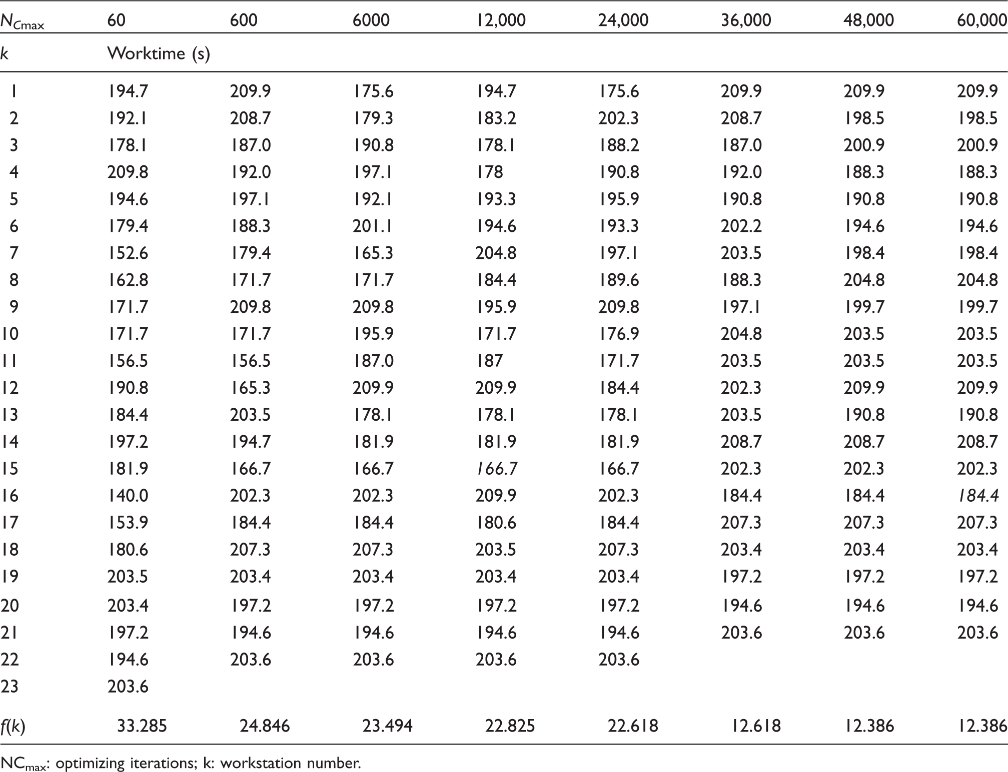
In this section, N was 65 and C was 210 s. The worktime at workstation k in Section-I and its variations with optimizing iterations (N_C_max) are presented in Table 4.

Table 4.

Worktime and iterations in AAC optimization of Section-I

N_C _max	60	600	6000	12,000	24,000	36,000	48,000	60,000
k	Worktime (s)
1	194.7	209.9	175.6	194.7	175.6	209.9	209.9	209.9
2	192.1	208.7	179.3	183.2	202.3	208.7	198.5	198.5
3	178.1	187.0	190.8	178.1	188.2	187.0	200.9	200.9
4	209.8	192.0	197.1	178	190.8	192.0	188.3	188.3
5	194.6	197.1	192.1	193.3	195.9	190.8	190.8	190.8
6	179.4	188.3	201.1	194.6	193.3	202.2	194.6	194.6
7	152.6	179.4	165.3	204.8	197.1	203.5	198.4	198.4
8	162.8	171.7	171.7	184.4	189.6	188.3	204.8	204.8
9	171.7	209.8	209.8	195.9	209.8	197.1	199.7	199.7
10	171.7	171.7	195.9	171.7	176.9	204.8	203.5	203.5
11	156.5	156.5	187.0	187	171.7	203.5	203.5	203.5
12	190.8	165.3	209.9	209.9	184.4	202.3	209.9	209.9
13	184.4	203.5	178.1	178.1	178.1	203.5	190.8	190.8
14	197.2	194.7	181.9	181.9	181.9	208.7	208.7	208.7
15	181.9	166.7	166.7	166.7	166.7	202.3	202.3	202.3
16	140.0	202.3	202.3	209.9	202.3	184.4	184.4	184.4
17	153.9	184.4	184.4	180.6	184.4	207.3	207.3	207.3
18	180.6	207.3	207.3	203.5	207.3	203.4	203.4	203.4
19	203.5	203.4	203.4	203.4	203.4	197.2	197.2	197.2
20	203.4	197.2	197.2	197.2	197.2	194.6	194.6	194.6
21	197.2	194.6	194.6	194.6	194.6	203.6	203.6	203.6
22	194.6	203.6	203.6	203.6	203.6
23	203.6
f(k)	33.285	24.846	23.494	22.825	22.618	12.618	12.386	12.386

NC_max: optimizing iterations; k: workstation number.

Table 4 lists the optimization results of different N_C_max. With the increase in iterations, the number of workstations, K, was reduced from 23 to 21, the objective function f(k) was gradually optimized to a minimal value (12.386), and the operation time of all the workstations was closer to the cycle time (210 s). The AAC optimization results indicated that all the operation tasks could be assigned to 21 workstations with an SI of 12.386. The lowest worktime, 184.4 s, among all the workstations occurred at the 16^th workstation where the corresponding idle time was 25.6 s. The company used to assign the Section-I tasks across 22 workstations based on the supervisors’ experience. Figure 3 shows the difference in the worktime at each workstation between the AAC and the supervisor’s experience in Section-I. It can be seen that the lowest worktime of all the workstations was 165.4 s at Workstation 13 where idle time was 44.6 s. The AAC optimization not only reduced the total number of workstations from 22 to 21 but also decreased the largest idle time from 44.6 s to 25.6 s.

Figure 3.

Section-I ALB solutions by AAC and the supervisor’s experience.

The one-piece flow assembly line for manufacturing Section-I (front body) is illustrated in Figure 4 according to the results of the AAC optimization, in which W_k, T_i and M_j denote workstation k, task i, and machine type j. In Section-I, 65 tasks were distributed across 21 workstations where 21 workers were employed to operate 11 different types of machines. Thirteen workstations housed two types of machine, and eight workstations housed one type of machine. For example, two types of machines, M₁: sewing machine and M₂: steam iron, were used in the first workstation (W₁) to perform three tasks, M₁ for T₉ (sewing pocket flap) and M₂ for T₁ (pressing front waist dart) and T₈ (pressing pocket facing). In the assembly line, a handwork task can be completed in the machine of the previous or next task.

Figure 4.

One-piece flow of Section-I.

Suit Section-II

In this case, N was 43. Table 5 lists the worktime of all the workstations in Section-II and its changes with optimizing iterations (N_C_max).

Table 5.

Worktime and iterations in AAC optimization of Section-II

N_C _max	60	600	6000	12,000	24,000	36,000	48,000	60,000
k	Worktime (s)
1	206.2	194.7	210.0	208.7	206.2	198.6	198.6	198.6
2	188.3	199.8	207.4	208.7	201.0	199.7	199.7	199.7
3	133.6	133.6	184.4	184.4	194.6	203.5	203.5	203.5
4	162.8	162.8	197.2	197.2	197.2	197.2	197.2	197.2
5	156.4	194.6	190.8	190.8	190.8	190.8	190.8	190.8
6	206.1	167.9	199.7	199.7	199.7	199.7	199.7	199.7
7	136.1	136.1	183.2	183.2	183.2	183.2	183.2	183.2
8	183.2	183.2	207.3	207.3	207.3	207.3	207.3	207.3
9	207.3	207.3	202.2	202.2	202.2	202.2	202.2	202.2
10	202.2	202.2
f(k)	42.055	40.817	15.228	15.216	13.974	13.757	13.757	13.757

NC_max: optimizing iterations; k: workstation number.

With the increase of iterations, the number of workstations in Section-II was reduced from 10 to 9, the objective function f(k) was gradually optimized to a minimal value (13.757). The lowest worktime, 183.2 s, occurred at the 7^th workstation where the corresponding idle time was 26.8 s. Figure 5 shows the difference in the worktime at each workstation between the AAC and the supervisor’s experience in Section-II. The company used to assign the tasks in Section-II across 10 workstations based on the supervisors’ experience. The lowest worktime of all the workstations was 133.6 s at Workstation 3 where the idle time was 76.4 s. The AAC optimization reduced the total number of workstations from 10 to 9 and decreased the largest idle time from 76.4 s to 26.8 s.

Figure 5.

Section-II ALB solutions by AAC and the supervisor’s experience.

Based on the AAC optimization, the one-piece flow assembly line for manufacturing Section-II (back body and collar) was illustrated in Figure 6, in which 43 tasks were distributed across nine workstations where nine workers were employed to operate six different types of machines. Each workstation housed two different machines. The first three workstations had a slightly larger number of tasks, and the total worktimes for W₁, W_2, and W₃ were 198.6 s, 199.7 s, and 203.5 s, respectively. More skillful workers were recommended for undertaking the tasks at these workstations.

Figure 6.

One-piece flow of Section-II.

Suit Section-III

The number of tasks in Section-III was 33. Table 6 presents the changes in worktime at each workstation when optimizing iteration (N_C_max) was increased. The number of workstations in Section-III was reduced from 12 to 11, the objective function f(k) gradually reached a minimal value (18.125). The lowest worktime (176.8 s) occurred at the 5^th workstation where the corresponding idle time was 33.2 s. Figure 7 shows the difference in worktime at each workstation between the AAC and the supervisor’s experience in Section-III. The company used to assign the tasks in Section-III across 12 workstations based on the supervisors’ experience. The lowest worktime of all the workstations was 118.4 s at Workstation 5 where the idle time was 91.6 s. AAC optimization reduced the total number of workstations from 12 to 11, and decreased the largest idle time from 91.6 s to 33.2 s.

Figure 7.

Section-III ALB solutions by AAC and the supervisor’s experience.

Table 6.

Worktime and iterations in AAC optimization of Section-III

N_C _max	60	600	6000	12,000	24,000	36,000	48,000	60,000
k	Worktime (s)
1	183.2	208.6	200.9	195.9	195.9	195.9	195.9	195.9
2	183.1	170.4	178.1	183.1	183.1	183.1	183.1	183.1
3	165.3	207.3	207.3	207.3	207.3	207.3	207.3	207.3
4	150.1	199.7	199.7	199.7	199.7	199.7	199.7	199.7
5	104.3	176.8	176.8	176.8	176.8	176.8	176.8	176.8
6	176.8	207.4	207.4	207.4	207.4	207.4	207.4	207.4
7	207.4	203.5	203.5	203.5	203.5	203.5	203.5	203.5
8	203.5	187.0	187.0	187.0	187.0	187.0	187.0	187.0
9	187.0	187.0	187.0	187.0	187.0	187.0	187.0	187.0
10	187.0	190.8	190.8	190.8	190.8	190.8	190.8	190.8
11	190.8	210.0	210.0	210.0	210.0	210.0	210.0	210.0
12	210.0
f(k)	41.612	19.683	18.566	18.125	18.125	18.125	18.125	18.125

NC_max: optimizing iterations; k: workstation number.

The one-piece flow assembly line for manufacturing Section-III (sleeve) is illustrated in Figure 8, in which 33 tasks are assigned to 11 workstations. Workstations 1 to 9 (W₁… W₉) housed two machines, W₁₁ housed one machine, and one workstation (W₁₁) required handwork. The worktimes at W₃, W₆, and W₁₁ were 207.3 s, 207.4 s, and 210 s, respectively, which were all close to the cycle time (210 s). The tasks at these workstations were more labor-intensive.

Figure 8.

One-piece flow of Section-III.

Skirt

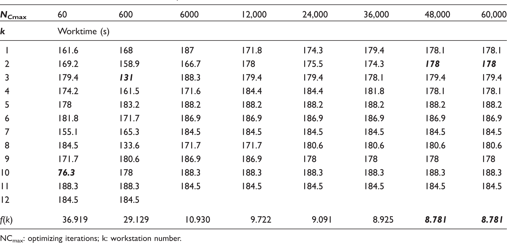
The number of tasks in this skirt production was 34, C was 190 s. Table 7 lists the changes in worktime at each workstation when the AAC optimizing iteration (N_C_max) was increased.

Table 7.

Worktime and iterations in AAC optimization of skirt

N_C _max	60	600	6000	12,000	24,000	36,000	48,000	60,000
k	Worktime (s)
1	161.6	168	187	171.8	174.3	179.4	178.1	178.1
2	169.2	158.9	166.7	178	175.5	174.3	178	178
3	179.4	131	188.3	179.4	179.4	178.1	179.4	179.4
4	174.2	161.5	171.6	184.4	184.4	181.8	178.1	178.1
5	178	183.2	188.2	188.2	188.2	188.2	188.2	188.2
6	181.8	171.7	186.9	186.9	186.9	186.9	186.9	186.9
7	155.1	165.3	184.5	184.5	184.5	184.5	184.5	184.5
8	184.5	133.6	171.7	171.7	180.6	180.6	180.6	180.6
9	171.7	180.6	186.9	186.9	178	178	178	178
10	76.3	178	188.3	188.3	188.3	188.3	188.3	188.3
11	188.3	188.3	184.5	184.5	184.5	184.5	184.5	184.5
12	184.5	184.5
f(k)	36.919	29.129	10.930	9.722	9.091	8.925	8.781	8.781

NC_max: optimizing iterations; k: workstation number.

After the iterations reached 48,000, the operation time of all the workstations was close to the cycle time (190 s). The number of workstations, K, was reduced from 12 to 11, the minimal value of the objective function f(k) was optimized at 8.781. The lowest worktime, 178 s, appeared at both the 2^nd and 9^th workstations where the corresponding idle time was 12 s. Figure 9 shows the difference in the worktime at each workstation when the task assignment was based on the AAC result and the supervisor’s experience, respectively. It can be seen that the lowest worktime of all the workstations was 133.5 s at Workstation 10 where the idle time was 56.5 s. The AAC optimization reduced the total number of workstations from 12 to 11, and decreased the largest idle time from 56.5 s to 12 s on the skirt assembly line.

Figure 9.

Skrit ALB solutions by AAC and supervisor’s experience.

In this one-piece flow assembly line, all the operation tasks could be assigned to 11 workstations with an SI being 8.781, as seen in Figure 10. Workstations 1 to 7 (W₁… W₇) and 10 (W₁₀) housed two machines, the rest housed one machine. The worktimes at all the workstations were close to the cycle time (190 s), especially at workstations 5 (188.2 s) and 10 (188.3 s). More skillful workers would be needed at these two workstations due to the shorter idle times.

Figure 10.

One-piece flow of skirt production.

Results and discussion

The analysis of variance (ANOVA) between the AAC optimized data and the company’s historical data was performed using IBM SPSS Statistics 21. The significance level (α) was set at 0.05. The results are shown in Table 8.

Table 8.

ANOVA between ACC optimized data and factory historical data

Source of variation	SS	df	MS	F	p
Suit Section-I
Between	885.879	1.000	885.879	6.885	0.012
Within	5275.673	41.000	128.675
Total	6161.551	42.000
Suit Section-II
Between	1857.448	1.000	1857.448	4.485	0.049
Within	7040.072	17.000	414.122
Total	8897.520	18.000
Suit Section-III
Between	1520.439	1	1520.439	4.002	0.059
Within	7978.986	21	379.952
Total	9499.424	22
Skirt
Between	1323.591	1	1323.591	9.354	0.006
Within	2971.635	21	141.506
Total	4295.226	22

SS: sum of squared error; MS: mean squared error; df: degree of freedom; F: F-value; p: p-value.

It was noted that the p-values for these significance tests were equal to 0.012 in Section-I, 0.049 in Section-II, and 0.006 for the skirt, which were below the significance level α = 0.05. Therefore, statistically there was a significant difference between the results from the AAC optimization and the supervisor’s experience in the three assembly lines. The p-value was 0.059 in Section-III, which was above the α level, thus, there was no significant difference between these two sets of data.

The load rate, F, of a workstation was calculated by dividing the worktime of a workstation by the cycle time; the assembly line arrangement efficiency, E, was measured by the average worktime divided by the maximum worktime of all the workstations. The lowest load rate (F), the number of workstations (K), the SI and the assembly line arrangement efficiency (E) in each assembly line are summarized in Table 9.

Table 9.

F, K, SI, E in each assembly line

	Suit Section-I		Suit Section-II		Suit Section-III		Skirt
	AAC	Historical	AAC	Historical	AAC	Historical	AAC	Historical
F	87.8%	78.8%	87.2%	63.6%	84.2%	56.3%	93.7%	70.3%
	(W16)	(W13)	(W7)	(W5)	(W5)	(W5)	(W2, W9)	(W10)
K	21	22	9	10	11	12	11	12
SI	12.386	23.799	13.757	40.900	18.125	38.984	8.781	27.548
E	95.2%	91.4%	95.7%	86.0%	93.0%	85.2%	95.9%	87.9%

F: the load rate; K: the number of workstations; SI: the smoothness index; E: the assembly line arrangement efficiency.

The advantage of the AAC data over the factory historical data is shown in Table 9. The AAC optimization increased the lowest load rate of workstation from 78.8% to 87.8% in Section-I, from 63.6% to 87.2% in Section-II, from 56.3% to 84.2% in Section-III, and from 70.3% to 93.7% in skirt. The reduction in the number of workstations was 4.5% in Section-I, 10.0% in Section-II, 8.3% in Section-III and 8.3% in skirt. The SI was reduced from 23.799 to 12.386 in Section-I, from 40.900 to 13.757 in Section-II, from 38.984 to 18.125 in Section-III, and from 27.548 to 8.781 in skirt. The assembly line arrangement efficiency was also improved from 91.4% to 95.2% in Section-I, from 86.0% to 95.7% in Section-II, from 85.2% to 93.0% in Section-III, and from 87.9% to 95.9% in skirt. These results demonstrate that the solutions from the AAC algorithm were quite effective.

The results of the AAC algorithm provided a basis for the company to redesign the assembly lines. By implementing the AAC solutions at the company, the supervisors can consider the operation tasks of different pieces in parallel, significantly improving the arrangement efficiency. Feedback from the factory was also constructive for improving the AAC. For example, if the number of tasks in a workstation was greater than six, more adaptation from workers performing different tasks was required, prolonging the theoretical operation time of the workstation. In the future, we will continue to advance the AAC to improve its operability by including more labor factors, such as the change time between different tasks.

Conclusions

In this paper, an AAC algorithm was presented to balance the one-piece flow assembly line of apparel production by rearranging mandatory tasks between workstations to maximize the worktime of each workstation. The AAC algorithm included modifications for estimating heuristic information, task probability, and pheromone update, which made it robust in searching for a global optimal solution and time-efficient in the optimizing convergence. Compared with using human experience to manually arrange tasks for suit and skirt production, AAC helped the company to reduce the number of workstations and cut idle time at most of them. The AAC should be suitable for solving other kinds of ALB problems.

Footnotes

Acknowledgement

The authors are grateful to the company who provided the production data and insights for this research.

Declaration of conflicting interests

The authors declare no potential conflicts of interest with respect to the research, authorship, and/or publication of this article.

Funding

The authors received no financial support for the research, authorship and/or publication of this article.

References

Chen

, et al. Assembly line balancing in garment industry. Expert Syst Appl 2012; 39: 10073–10081.

Chan

KCC

Hui

PCL

Yeung

. Handling the assembly line balancing problem in the clothing industry using a genetic algorithm. Int J Cloth Sci Tech 1998; 10: 21–37.

Protzman

McNamara

Protzman

. One-piece flow vs. batching: A guide to understanding how continuous flow maximizes productivity and customer value, Boca Raton, FL: CRC Press, 2016, pp. 3–8.

Kumar

. Value stream mapping-a lean manufacturing approach to reduce the process wastages in clothing industry. IJAME 2016; 5: 23–33.

Miltenburg

. One-piece flow manufacturing on U-shaped production lines: a tutorial. IIE Trans 2001; 33: 303–321.

Rong

. The reliable design of one-piece flow production system using fuzzy ant colony optimization. Comput Oper Res 2009; 39: 1656–1663.

Shook

Marchwinski

. Lean lexicon: A graphical glossary for lean thinkers, 5th ed. Cambridge, MA: Lean Enterprise Institute, 2014, pp. 5–10.

Satoglu

Durmusoglu

Ertay

. A mathematical model and a heuristic approach for design of the hybrid manufacturing systems to facilitate one-piece flow. Int J Prod Res 2010; 48: 5195–5220.

Stockton

Ardon-Finch

Khalil

. Walk cycle design for flexible manpower lines using genetic algorithms. Int J Comput Integ Manuf 2005; 18: 15–26.

10.

Make

MRA

Rashid

MFFA

Razali

. A review of two-sided assembly line balancing problem. Int J Adv Manuf Tech 2017; 89: 1743–1763.

11.

Kara

Gökçen

Atasagun

. Balancing parallel assembly lines with precise and fuzzy goals. Int J Prod Res 2010; 48: 1685–1703.

12.

Ünal

Tunali

Güner

. Evaluation of alternative line configurations in apparel industry using simulation. Text Res J 2009; 79: 908–916.

13.

Liu

Ong

. Branch-and-bound algorithms for simple assembly line balancing problem. Int J Adv Manuf Tech 2008; 36: 169–177.

14.

Scholl

Klein

. SALOME: a bidirectional branch and bound procedure for assembly line balancing. INFORMS J Comput 1997; 9: 319–334.

15.

Vilà

Pereira

. A branch-and-bound algorithm for assembly line worker assignment and balancing problems. Comput Oper Res 2014; 44: 105–114.

16.

Kao

EPC

. A preference order dynamic program for stochastic assembly line balancing. Manage Sci 1976; 22: 1097–1104.

17.

Ahmad

Yousaf

. Manufacturer oriented mixed model assembly line scheduling using dynamic programming. VAWKUM Trans Comput Sci 2015; 6: 7–15.

18.

Esmaeilbeigi

Naderi

Charkhgard

. The type E simple assembly line balancing problem: a mixed integer linear programming formulation. Comput Oper Res 2015; 64: 168–177.

19.

Talbot

Patterson

. An integer programming algorithm with network cuts for solving the assembly line balancing problem. Manage Sci 1984; 30: 85–99.

20.

Özcan

Toklu

. A tabu search algorithm for two-sided assembly line balancing. Int J Adv Manuf Tech 2009; 43: 822–829.

21.

Chan

KCC

Hui

PCL

Yeung

, et al. Handling the assembly line balancing problem in the clothing industry using a genetic algorithm. Int J Cloth Sci Tech 1998; 10: 21–37.

22.

Alavidoost

Zarandi

MHF

Tarimoradi

. Modified genetic algorithm for simple straight and U-shaped assembly line balancing with fuzzy processing times. J Intell Manuf 2017; 28: 313–336.

23.

Güden

Meral

. An adaptive simulated annealing algorithm-based approach for assembly line balancing and a real-life case study. Int J Adv Manuf Tech 2016; 84: 1539–1559.

24.

Zhong

. A modified ant colony optimization algorithm for multi-objective assembly line balancing. Soft Comput 2017; 21: 6881–6894.

25.

Dorigo

Maniezzo

Colorni

. The ant system: optimization by a colony of cooperating agents. IEEE Trans Syst Man Cybern B Cybern 1996; 26: 29–41.

26.

Hasan

AlKhamis

Ali

. A comparison between simulated annealing, genetic algorithm and Tabu search methods for the unconstrained quadratic Pseudo-Boolean function. Comput Ind Eng 2000; 38: 323–340.

27.

Alhamdy

SAS

Noudehi

Majdara

. Solving traveling salesman problem (TSP) using ants colony (ACO) algorithm and comparing with Tabu search, simulated annealing and genetic algorithm. J Appl Sci Res 2012; 1: 434–440.

28.

McMullen

Tarasewich

. Using ant techniques to solve the assembly line balancing problem. IIE Trans 2003; 35: 605–617.

29.

Bautista J and Pereira J. Ant algorithms for assembly line balancing. In: Proceedings third international workshop on ant algorithms (ed initial last name), Brussels, Belgium, 12 September–14 September, 2002, pp. 65–75. Berlin, Heidelberg: Springer.

30.

Bautista

Pereira

. Ant algorithms for a time and space constrained assembly line balancing problem. Eur J Oper Res 2007; 177: 2016–2032.

31.

Sabuncuoglu

Erel

Alp

. Ant colony optimization for the single model U-type assembly line balancing problem. Int J Prod Econ 2009; 120: 287–300.

32.

Baykasoğlu

Dereli

. Simple and U-type assembly line balancing by using an ant colony based algorithm. Math Comput Appl 2009; 14: 1–12.

33.

Yagmahan

. Mixed-model assembly line balancing using a multi-objective ant colony optimization approach. Expert Syst Appl 2011; 38: 12453–12461.

34.

Zha

. A hybrid ant colony algorithm for U-line balancing and rebalancing in just-in-time production environment. J Manuf Syst 2014; 33: 93–102.

35.

Kalayci

. Assembly line balancing using an ant algorithm in the garment industry: a case study. Text Sci Econ 2015, pp. 14–17.

36.

Zhong

. A modified ant colony optimization algorithm for multi-objective assembly line balancing. Soft Comput 2017; 21: 6881–6894.

37.

Chen JC, Hsaio MH, Chen CC, et al. A grouping genetic algorithm for the assembly line balancing problem of sewing lines in garment industry. In: Proceedings of the eighth international conference on machine learning and cybernetics Hebei, China, 12–15 July, 2009, pp. 2811–2816. USA: IEEE.

38.

Tasan

Tunali

. A review of the current applications of genetic algorithms in assembly line balancing. J Intell Manuf 2008; 19: 49–69.

39.

Hou

Lai

, et al. Product family assembly line balancing based on an improved genetic algorithm. Int J Adv Manuf Tech 2014; 70: 1775–1786.

40.

Miltenburg

Wijngaard

. The U-line line balancing problem. Manage Sci 1994; 40: 1378–1388.

41.

Boysen

Fliedner

Scholl

. A classification of assembly line balancing problems. Eur J Oper Res 2007; 183: 674–693.

42.

Khosravi

Sadeghi

Jolai

. An improvement in calculation method for apparel assembly line balancing. Indian J Fibre Text Res 2013; 38: 259–264.

43.

Kayar

Bulur

ÖC

. Study on the importance of employee performance assessment and lost productive time rate determination in garment assembly lines. Fibres Text East Eur 2017; 25: 119–126.

44.

Tao

Zhang

, et al. Ant colony optimization algorithm for balancing mixed-model assembly line. Modular Machine Tool & Automatic Manufacturing Technique 2011; 2: 32–35.