Modeling fiber arrangement and distribution during the roller drafting process

Abstract

During the spinning process, the roller drafting operation plays a significant role in attenuating the sliver to an appropriate linear density. In this study, the model of fiber arrangement was applied to simulating the roller drafting process in order to shed light on the sliver dynamic behavior in the drafting zone. The drafting process was operated from the high-velocity motion of the first accelerated fiber to the high-velocity motion of the last accelerated fiber. The proposed model showed that the simulated sliver attenuation processes were highly corresponded to the actual sliver attenuation results. In addition, the results revealed that the draft ratio, gauge length, input sliver linear density and accelerated-point distribution form had effective influences on the attenuation curves of sliver linear density, whilst the delivery speed scarcely had any effect. The fiber distributions of various forms were also investigated specifically and quantitatively from the fiber arrangement during the drafting procedure in real time. Furthermore, the sliver dynamic was also described by the mean and CV of fiber velocities within the drafting zone. The obtained simulation results demonstrated that the draft ratio, gauge length and delivery speed had a bearing on the mean velocity of fibers, while the CV of fiber velocities was significantly influenced by the draft ratio, gauge length and input sliver linear density. Besides, the distribution pattern has a valuable contribution to the mean and CV of fiber velocities. In consequence, the new drafting model was validated to be effective in quantizing the drafting process.

Keywords

roller drafting fiber arrangement attenuation curve fiber distribution fiber velocity

Roller drafting is an indispensable and essential procedure in the yarn forming process, which attenuates slivers to an appropriate linear density during the spinning process. The relationship between drafting parameters and sliver irregularity has attracted the attention of researchers, who have studied drafting by theoretical and experimental approaches. Among them, Rao¹ elaborated the description of the ideal sliver and studied the effect of roller drafting on the structure of the ideal sliver. Essentially, it is fiber motion in the drafting zone that exerts the effect on sliver evenness. Since the suggestion of instantaneous acceleration of the floating fiber by Taylor,^2,3 there have been many studies of floating fiber motion. Weber and Wulfhorst⁴ focused on the acceleration of the floating fiber by observation of the tracer fibers. The floating fiber motion was theoretically simulated by Yao et al.⁵ and the statistics of accelerated points were analyzed by the forces acting on it. Recently, Yan and Yu⁶ described the accelerated-point distribution of floating fibers by a parabolic density. The log-normal distribution was given to fit the accelerated-point distribution of floating fibers during the roller drafting process by Lin et al.^7,8

Furthermore, the drafting process has also been simulated by many mathematical and computer models. An assumed random sliver and fiber end distribution were applied in the computer simulation by Johnson.⁹ Huh and Kim^10–12 tried to formulate and simulate the dynamic behavior of a fiber bundle in the roller drafting and derive the attenuation curves of linear density. Kim et al.^13–16 also analyzed the sliver thickness variation and fiber behavior theoretically. Later, a discrete-event simulation model of one-dimensional fibrous material was applied in the simulation of the roll-drafting process elaborated by Cherkassky.^17,18 The work of Ma and Wang¹⁹ strongly improved the model by considering the movement time of individual fibers and gave out the variation tendency of the fiber number qualitatively in the drafting zone.

There is no doubt that all the studies contributed to analyzing the drafting process and sliver qualities. Nonetheless, the drafting procedure cannot be presented in real time and the specific fiber arrangement in the drafting zone cannot be depicted by previous researches. In order to investigate the array of different classifications of fibers and the sliver dynamic motion in the drafting zone for optimizing the drafting operation, however, an exact model of roller drafting is required. Therefore, in this study, our main objective is to apply the model of fiber arrangement in the sliver into the roller drafting simulation and realize the achievement of quantifying the drafting process. Then, in what follows, the drafting process with different drafting parameters can be expressed intuitively by fiber arrangement in real time. With this model, the sliver attenuation process and fiber velocity variation can be described from the fiber arrangement and distribution in the drafting area. Meanwhile, the simulated results were compared with the experimental ones to confirm the viability of the model.

Modeling

To employ the model of fiber arrangement in this drafting simulation, individual fibers in the sliver are assumed to be straightly parallel to the sliver axis firstly. In the drafting operation, it is assumed that the acceleration processes of all the fibers operate immediately. This means that their velocities change instantaneously from a lower speed – the velocity of the back roller – to a high speed – the velocity of the front roller during roller drafting. During the drafting process, the accelerated positions of fibers are unfixed, which usually follow some roles of the probability distribution. It should be noted that the simulation of acceleration distribution in the drafting model has involved an indirect expression for the influence of the friction on fiber behavior in the drafting zone. The friction between the fibers in the drafting zone is one of the main factors resulting in the acceleration distribution of floating fibers during the drafting process and it is seriously affected by the drafting parameters, such as the top roller pressure, drafting ratio, gauge length, input sliver linear density and so on. Besides, the modeling of fiber acceleration distribution can also indirectly reflect the effect of drafting force on the drafting process. It is understood that the drafting force is the friction force exerted on all the fast fibers when the fast fibers move out from the slow fibers.

Referring to Figure 1, the fiber arrangements of before, during and after drafting are described by the model of fiber arrangement. Firstly, the fiber arrangement in the sliver before the drafting process is provided when the nip line of the back roller is defined as the coordinate origin (0) along the sliver axis by the method of Jiang et al.²⁰ Fibers are randomly distributed in a sliver with a given length based on Uniform Distribution.²¹ The theory that the number of fiber heads in a given sliver segment submitted to Poisson Distribution has been proposed and applied in many researches.^22,23 For a prescribed sliver length l_s, the number of fibers in this sliver segment, n, is

n = \frac{N_{s} l_{s}}{N_{f} l_{f}}

(1)

where N_s is the sliver fineness; N_f is the mean fiber fineness; and l_f is the mean fiber length. Secondly, in regard to the drafting process, it starts from the high-velocity motion of the first fiber being accelerating and ends at the high-velocity motion of the last fiber being accelerating. Lastly, it is regarded as the end of the drafting process when all the fibers in the sliver accomplish the acceleration process and stay in the high-speed movement stage. The position of the first accelerated fiber when the drafting process ends is defined as the fresh coordinate origin (0′) along the sliver axis. In consequence, the fiber arrangement in the sliver can be obtained from the distance between the head of the fibers and this fresh coordinate origin (0′) during the drafting process.

Figure 1.

Schematic drawing of the drafting process.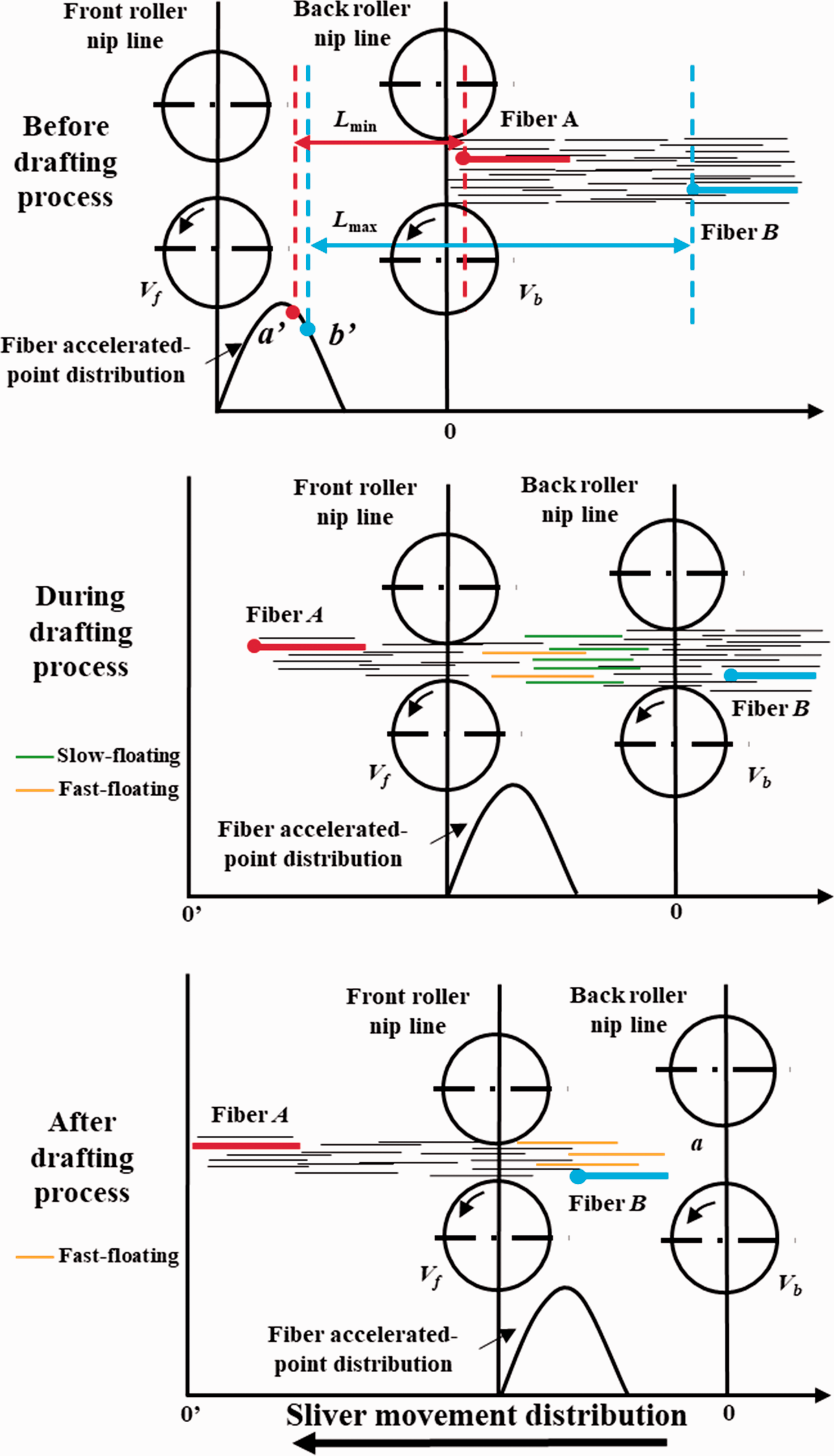

As depicted in Figure 1, suppose that fiber A is the first accelerated fiber, whose position away from its accelerated point, L_min, is the minimum distance among all fibers due to all fibers moving with the speed of the back roller before they accelerate to the speed of front roller. Fiber B is assumed to be the last accelerated fiber, whose position away from its accelerated point, L_max, is the maximum distance among all fibers. It is assumed that point a' is the accelerated position of fiber A and point b' is the accelerated position of fiber B. Then the drafting time, t, can be expressed as

t = t_{max} - t_{min} = \frac{L_{max} - L min}{V_{b}}

(2)

where V_b is the velocity of the back roller; t_min is the time of fiber A during the low-speed stable stage; and t_max is the time of fiber B during the low-speed stable stage. When the drafting process is accomplished, the moving distance of fiber A is

L_{a} = (t - t_{min}) V_{f} + t_{min} V_{b}

(3)

where V_f is the velocity of the front roller. Therefore, the distance of the fresh coordinate origin (0′) away from the old coordinate origin (0) can be obtained as

L_{0'} = L_{a} - l_{a}

(4)

where l_a is the distance between the head of fiber A before the drafting process and the old coordinate origin (0). Then the position of the head of every fiber during the drafting process can be divided into two cases as follows.

The fiber has not accelerated and moves at the lower speed, that is

\begin{array}{l} v_{i} = V_{b} \\ L_{i} = L_{0'} + l_{i} - v_{i} t_{j} \end{array}} t_{j} < \frac{l_{i} + x_{i}}{V_{b}}

(5)

The fiber has accelerated and moves at the higher speed, that is

\frac{\begin{matrix} v_{i} = V_{f} \\ L_{i} = L_{0'} - [t_{j} - (l_{i} + x_{i})] v_{i} + x_{i} \end{matrix} {t_{j} \geq l_{i} + x_{i}}{\begin{matrix} V_{b} \end{matrix}}

(6)

where subscript i indicates the fiber number in the sliver; L_i indicates the distance between the head of fiber i during the drafting process and the fresh coordinate origin (0′), that is, the fresh position of the head of fiber i during the drafting process; l_i indicates the distance between the head of fiber i before the drafting process and the old coordinate origin (0), that is, the old position of the head of fiber i before the drafting process; x_i indicates the distance between the accelerated point of fiber i and the nip line of the front roller; and t_j is the arbitrary time during drafting process. Then the fiber arrangement in the sliver during the drafting process can be depicted from the new positions of the fiber heads and fiber lengths, as shown in Figure 1. Besides, the fiber arrangement after the drafting simulation of one zone can be recorded as the input fiber arrangement for the next drafting zone. Hence, this drafting model can be similarly applied to simulate the fiber arrangement and distribution in the drafting systems of two or three zones.

Results and discussion

In order to simplify the simulation process, the drafting simulation of viscose was conducted to validate the drafting model due to its same length and fineness. Besides, this model is also suitable for other synthetic fibers and natural fibers, such as cotton, when the length distribution and fineness distribution are taken into consideration. In the actual drafting experiments, the parameters of viscose fiber were chosen as follows: l_f = 38mm, n_f = 1.33 dtex, and all the fibers have the same length and fineness. It is difficult to measure directly the sliver linear density in a draft zone. Therefore, the linear density profiles of slivers can be obtained by cutting and weighing the specimens by the length of 2 mm in the drafting zone when the drafting process is completed. In the drafting system, the speed of the front roller remains constant as the delivery speed and the speed of the back roller change with the draft ratio. In our experiments, four different drafting parameters, namely the draft ratio, gauge length, delivery speed and input sliver linear density, are given to check the effects on the sliver dynamic behavior during drafting (Table 1). It should be noted that the distance between the back and front rollers is generally 6–14 mm longer than the fiber length, so that the gauge lengths are chosen as 44, 46, 48, 50 and 52 mm when the fiber length is 38 mm. The delivery speeds were set as 10, 20 and 30 m/min due to our limited experimental conditions.

Table 1.

Experimental parameters in the drafting system

Draft ratio	3.67, 4.4, 5.13, 6.6, 7.33	5.13	5.13	5.13
Gauge length (mm)	48	44, 46, 48, 50, 52,	48	48
Delivery speed (m/min)	20	20	10, 20, 30	20
Input sliver linear density (tex)	4128	4128	4128	4128, 8256, 12,384

In the specific drafting simulation, the drafting parameters are input according to the experimental parameters and the accelerated points are randomly simulated based on the experimental value by the trace method introduced by Mupfudze et al.²⁴ Specifically speaking, the fiber accelerated points are calculated from the positions before and after drafting of the dyed tracer fibers embedded in the single sliver. For the simulation, the accelerated points of every fiber are randomly simulated based on the experimental histograms of fiber accelerated-point distribution by the Monte Carlo method. The calculation for simulated attenuation curves of sliver linear density in the drafting zone during the drafting process is similar to that of the test method. The simulated sliver linear density is the weight of fibers in every sliver segment of 1 mm, calculated from multiplying the fiber lengths by their fineness in the sliver segment. Furthermore, in order to compare the simulated with the tested results, the unit of “tex” was used for the sliver linear density in the draft zone in both simulated and tested results in all figures.

Sliver linear density profiles in the drafting zone

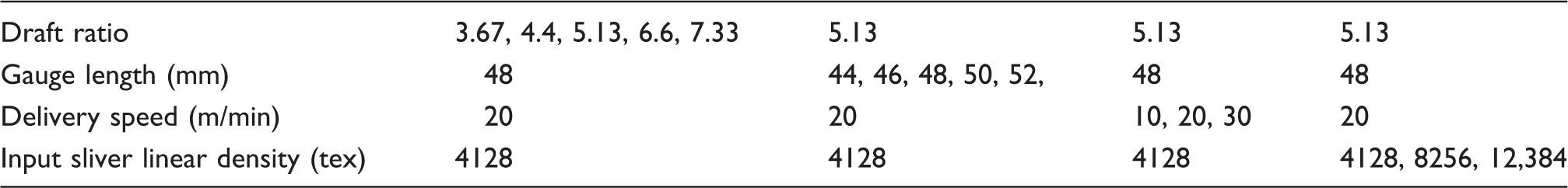
The simulation results for linear density with respect to time within the drafting area at any instant during the whole drafting process under the simulation conditions in which the draft ratio is 5.13, gauge length is 48 mm, delivery speed is 20 m/min and input sliver linear density is 4128 tex are given in Figure 2. The sliver linear density can be calculated from the fiber arrangement in the sliver during the drafting process. Obviously, it can be seen that the three-dimensional (3D) profile has a transient fluctuation state at the beginning of drafting time, then turns into a constant steady state, but demonstrates a transient unsteady state again at the end of drafting time. The unsteady states at the beginning and end of drafting time are mainly caused by the incompleteness of the head and tail of the sliver. Therefore, the simulated results at the same fixed time in the steady state were chosen to analyze and compare with the measured ones.

Figure 2.

The simulated attenuation curves of sliver linear density in the drafting zone during the drafting process.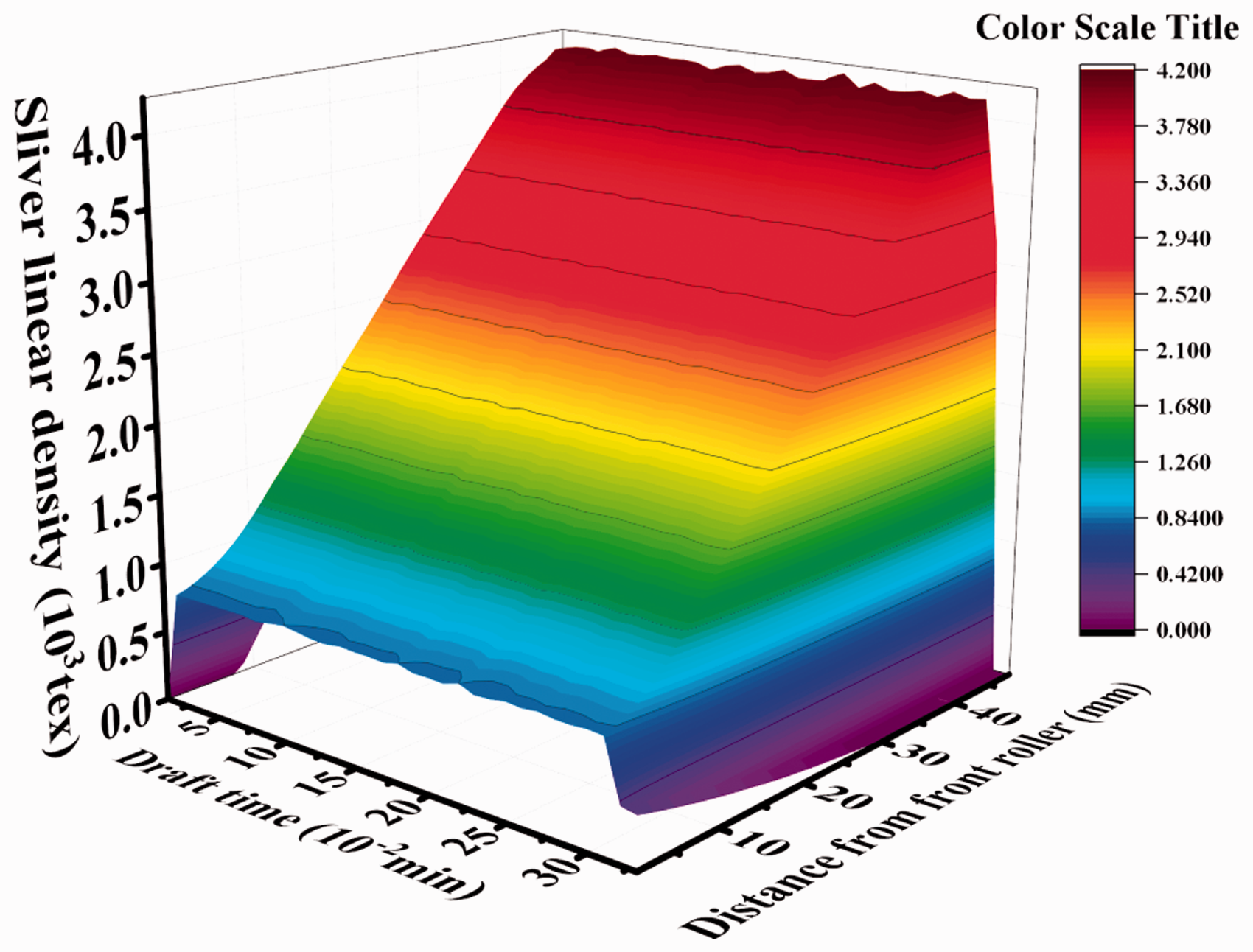

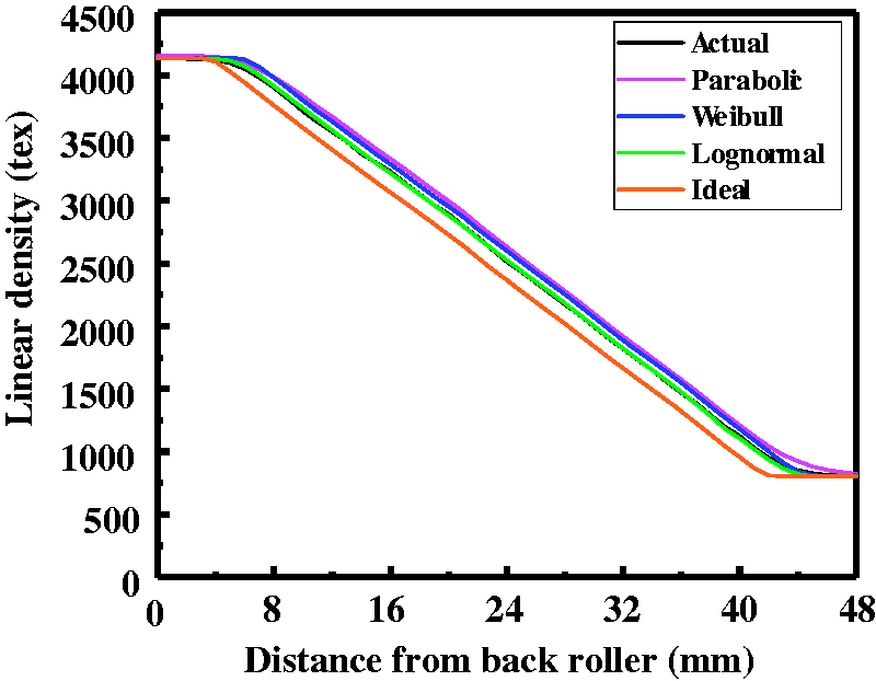
Besides, four kinds of distributions for fiber accelerated points used to simulated fiber accelerated points are compared with the simulated results of ideal accelerated points under the simulation conditions in which the draft ratio is 5.13, gauge length is 48 mm, delivery speed is 20 m/min and input sliver linear density is 4128 tex. The distributions for fiber accelerated points are shown in Figure 3. The ideal accelerated points of every fiber elaborated by Lin et al.⁷ are equal to G/(1 + D), where G is the gauge length and D is the draft ratio. The Parabolic density function was adopted to estimate the accelerated positions of fibers in the drafting zone.⁶ Weibull distribution and log-normal distribution were proposed by Lin et al.^7,8 to describe the accelerated points of fibers during the drafting procedure. The simulated attenuation curves of linear density are illustrated in Figure 4.

Figure 3.

Four kinds of distributions for fiber accelerated points.

Figure 4.

The simulated attenuation curves of sliver linear density under different accelerated-point distribution.

From the illustration in Figure 4, it can be seen that the simulated attenuation curves of sliver linear density with the distribution of accelerated points obviously varies from those with ideal accelerated points. Moreover, the attenuation processes simulated with the probability distributions of accelerated points are Parabolic, Weibull and log-normal, which are distinctly different from each other due to the diverse degrees of dispersion for the acceleration distribution in Figure 3. Besides, the simulated attenuation curves of sliver linear density with the actual and log-normal acceleration distribution are almost overlapping because of the similarity of these two probability distribution curves, as shown in Figure 3. Therefore, the result clearly indicates that distribution of fiber accelerated points has a significant effect on the attenuation process of sliver linear density. To enhance the accuracy of the simulated results, log-normal distribution was applied in the following simulated program.

Figure 5 shows the attenuation curves of linear density obtained from the above-mentioned drafting model, whilst the triangle-dot line curves denote the measured linear density according to the variations of drafting conditions. Even though the tested results deviate more or less from the simulated curves, they can be considered to be in accordance with each other. It is notable that the linear density of slivers in the drafting area decreases slowly from the back roller, but then begins to decline rapidly. Subsequently, it becomes relatively steady and finally reaches the output value when approaching the front roller. From Figure 5(a), it can be concluded that the attenuation rate of sliver linear density increases as the draft ratio increases if the other parameters kept constant. Similarly, the attenuated speed of sliver linear density has a growing tendency with the input linear density increasing for the same draft ratio, as shown in Figure 5(d). The simulated results are consistent with the conclusion obtained by Huh and Kim.^10,11 Besides, as shown in Figure 5(b), the attenuation curves are almost parallel each other when the distance is 16–40 mm from the back roller as the gauge length increases. This denotes that the slivers in the draft zone are attenuated at the same velocity with the increase of the distance separating the roller nips when the distance is 16–40 mm from the back roller. In contrast, the sliver linear density seems less related to the delivery speed, as described in Figure 5(c), which is in accordance with the results of Huh and Kim.¹¹ Moreover, the simulation results with different delivery speeds also indicate that the proposed drafting model can be similarly applied in simulating the fiber arrangement during the drafting process at much higher speed or other different practical conditions.

Figure 5.

The simulated and tested attenuation curves of sliver linear density in the drafting zone for various drafting conditions: (a) draft ratio; (b) gauge length; (c) delivery speed; (d) input sliver linear density.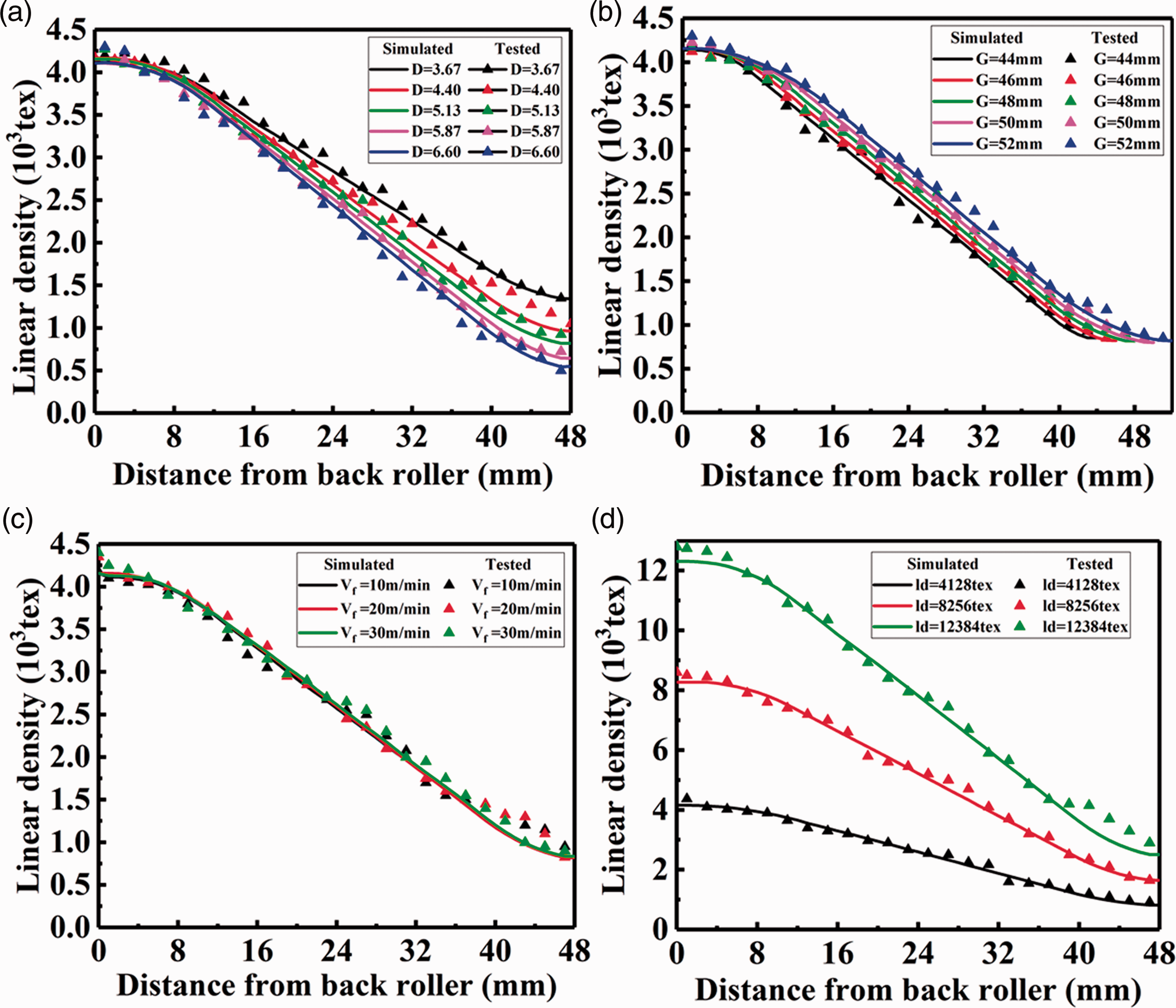

To sum up, in spite of the slight discrepancy, the good consistency between actual results and simulation results greatly validated the effectiveness of the model. Also, our study demonstrates that the proposed drafting model can approximate fairly well the attenuation curves of sliver linear density obtained from experiments. This indicates that the drafting model based on fiber arrangement can describe the sliver dynamic characteristics in the drafting zone during the drafting process. Concretely speaking, the sliver linear density in the drafting area substantially depends on the draft ratio, gauge length, input sliver linear density and distribution pattern of fiber accelerated points, but not delivery speed.

Fiber arrangement and distribution in the drafting zone

Based on the developed drafting model, the arrangement and distribution of various fibers under the condition that draft ratio is 5.13, gauge length is 48 mm, delivery speed is 20 m/min and input sliver linear density is 4128 tex are simulated to illustrate the dynamic behavior of fibers in the area between the front and back rollers.

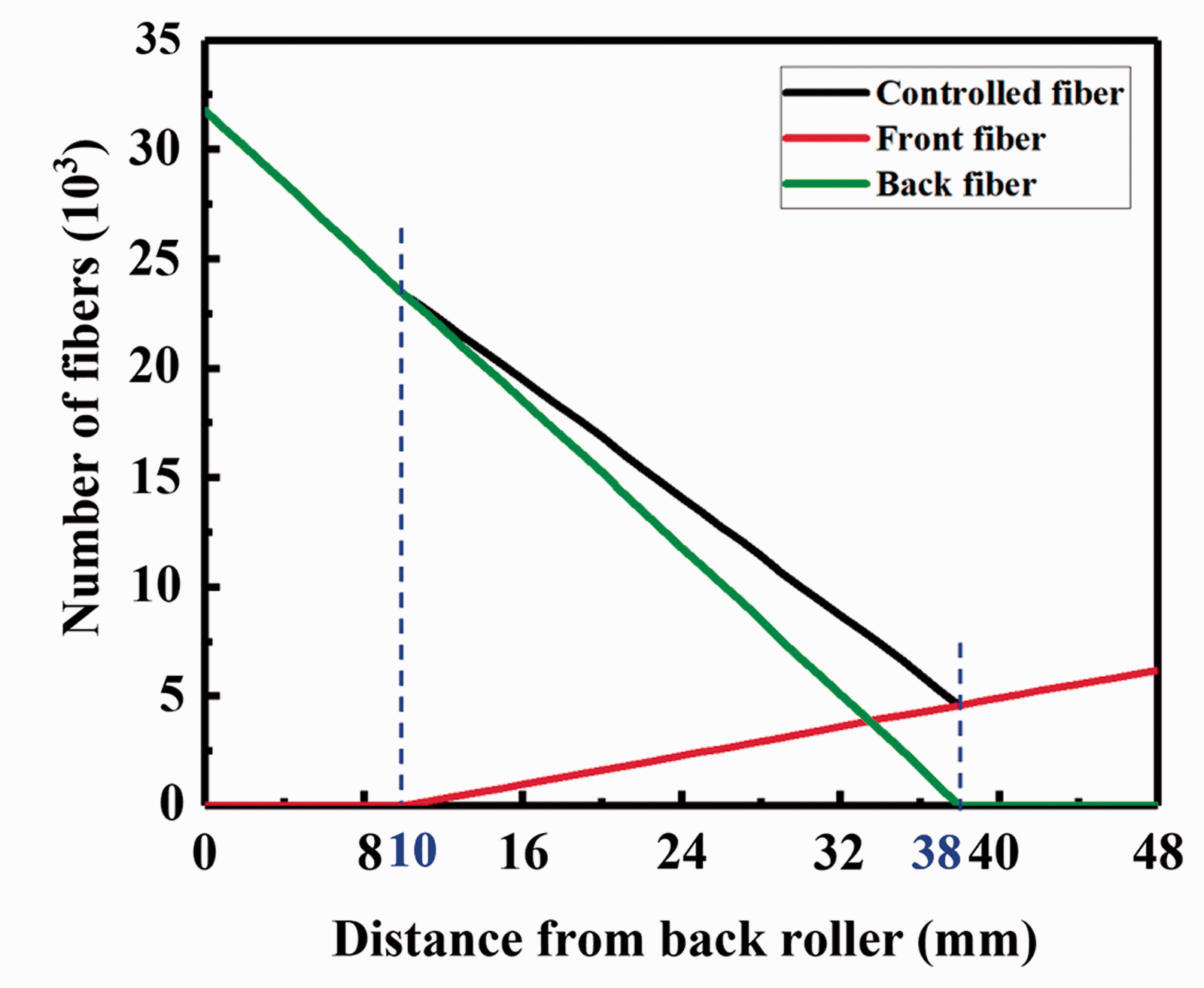
From Figure 6, it can be recognized that controlled and floating fibers are arranged in the sliver in the zone between the nip line of the front and back rollers. Controlled fibers consist of the fibers griped by the front roller and the back roller; it can be seen from Figure 7 that the distribution of fibers griped by the front roller and the back roller is related directly to fiber length (38 mm). The back fibers gradually decrease to 0 at 38 mm from the back roller, while the front fibers steadily reduce to 0 at 38 mm away from the front roller, so that the farther away from the roller nip line, the less controlled the fibers. Appreciably, there are significantly more fibers clamped by the back roller than fibers clamped by the front roller in the drafting area. Therefore, as shown in Figure 6, the controlled fibers reach the minimum at 38 mm away from the back roller, where the floating fibers begin to decline and the slope of decline reduces as the sliver approaches the front roller. From 0 to 38 mm away from the back roller, the floating fibers increase near the back roller and the slope of increase reduces to 0 at 10 mm away from the back roller, then remains steady.

Figure 6.

The arrangement and distribution of controlled and floating fibers in the drafting zone.

Figure 7.

The arrangement and distribution of front and back fibers in the drafting zone.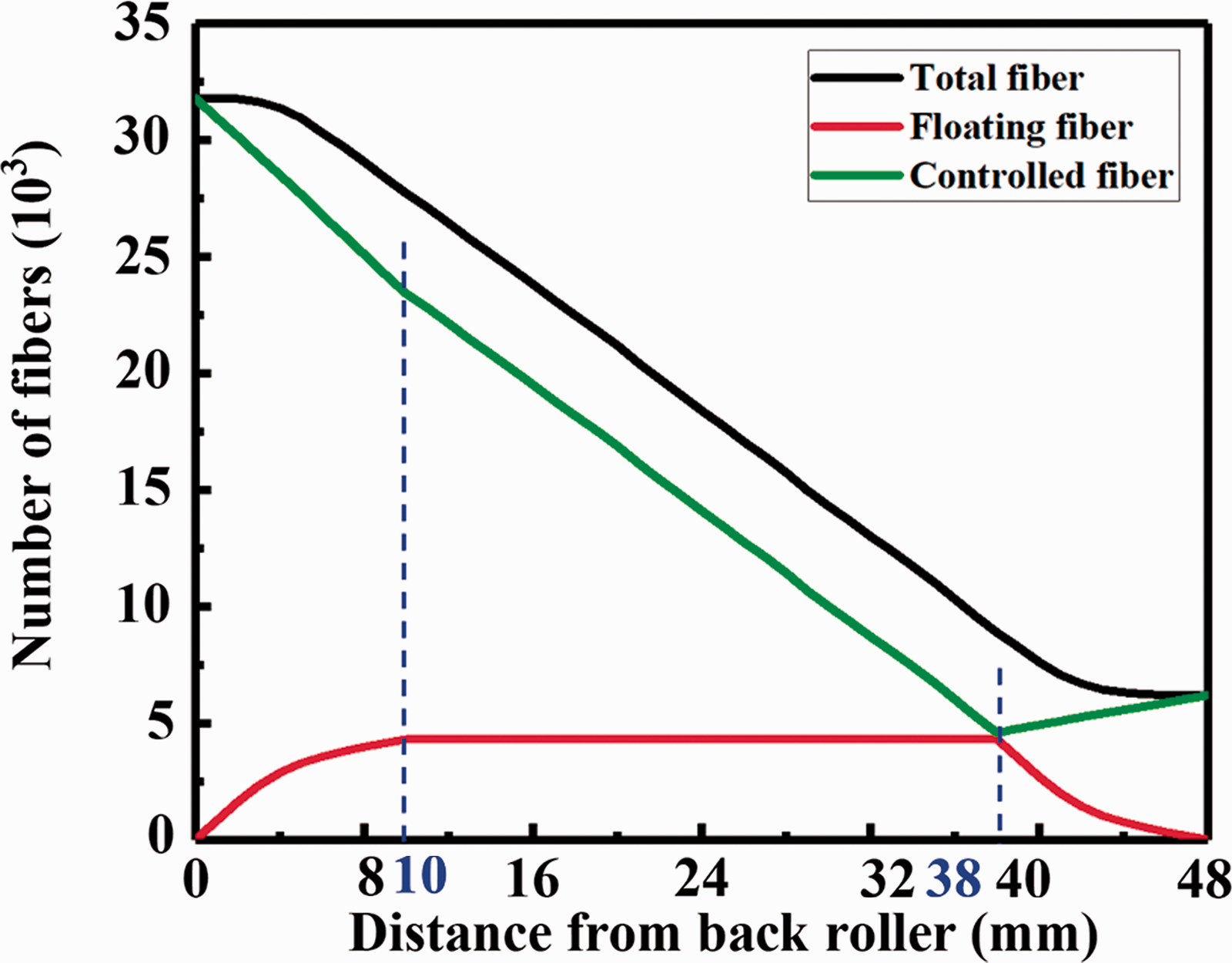

As shown in Figure 8, there are fast-floating fibers moving at the velocity of the front roller and slow-floating fibers moving at the velocity of the back roller in the drafting region. Obviously, the slow-floating fibers are the main portion of the floating fibers, while the fast-floating fibers are just a small part. Hence, the distribution of the floating fibers clearly reflects the moving situation of slow-floating fibers in the drafting zone, whose speed first increases rapidly near the back roller, then gradually becomes stable, and decreases drastically to 0 when the sliver reaches the front roller. For the fast-floating fibers, their speed first similarly remains steady from 10 to 38 mm away from the back roller, but then their increasing velocity grows little by little from 0 to 10 mm far away from the back roller and the decreased velocity gradually reduces from 38 to 48 mm away from the back roller.

Figure 8.

The arrangement and distribution of fast-floating and slow-floating fibers in the drafting zone.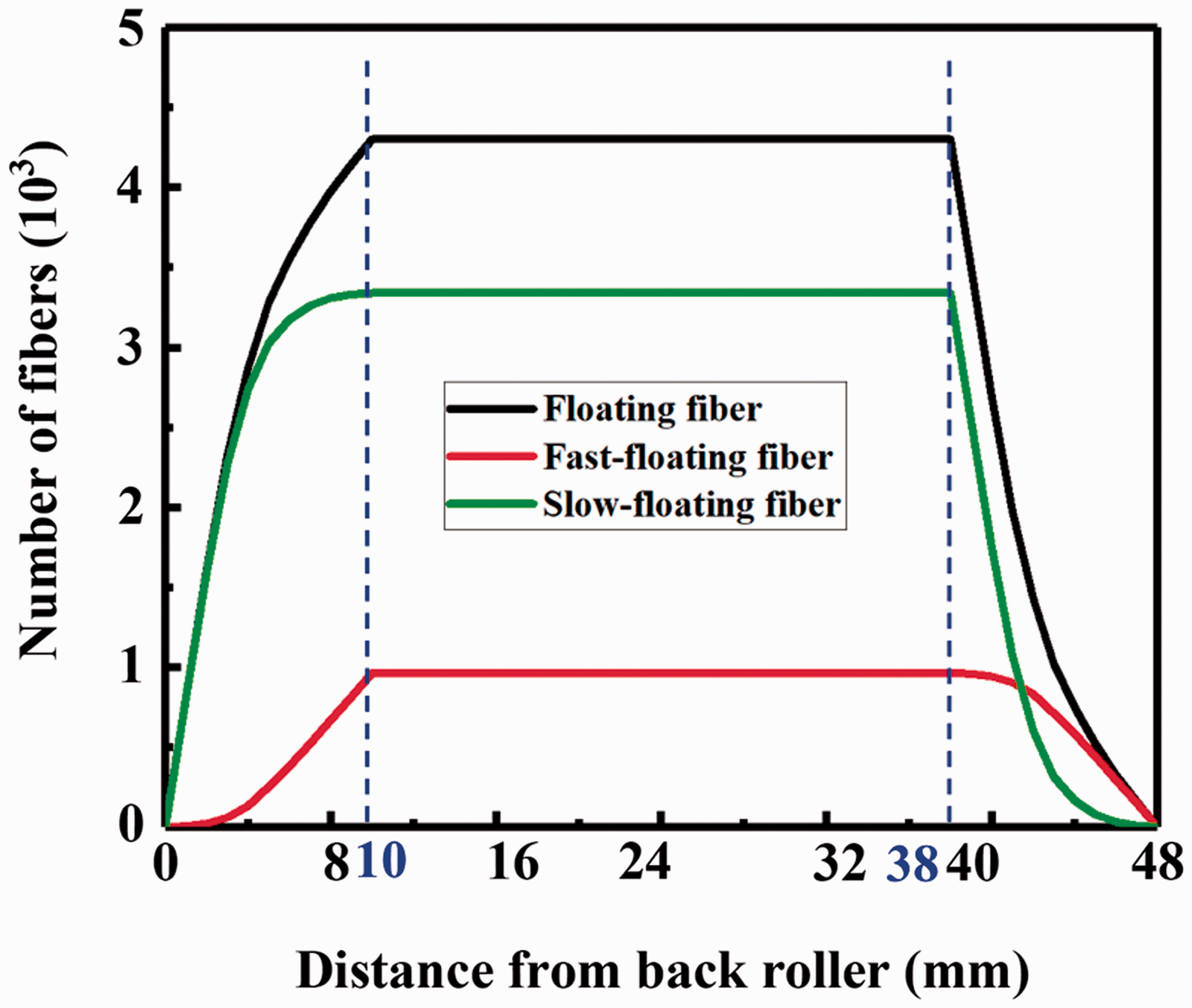

The arrangement and distribution of fast and slow fibers in the area between the nip line of the front and back rollers are presented in Figure 9. It can be seen that fast fibers consisted of front fibers and fast-floating fibers, while slow fibers are composed of back fibers and slow-floating fibers. The fast fibers decline on approaching the front roller, whilst slow fibers increase with the distance from the back roller. It is worth noting that slow fibers are the main part of the drafting area, which is similar to the simulation of Ma and Wang.¹⁹

Figure 9.

The arrangement and distribution of fast and slow fibers in the drafting zone.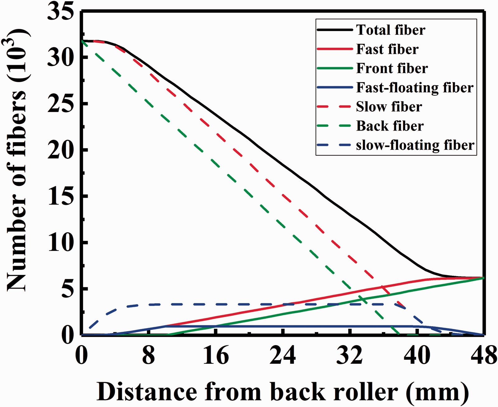

The velocity of fibers in the drafting zone

Based on the fiber distribution with different velocities in the drafting, the fiber motion in the drafting for various conditions can be revealed from the mean and CV of fiber velocities. As demonstrated in Figure 10, the simulation results illustrate a 3D relationship between the mean and CV of fiber velocities in the drafting zone with time. The simulation conditions are that the draft ratio is 5.13, gauge length is 48 mm, delivery speed is 20 m/min and input sliver linear density is 4128 tex. The incompleteness of the head and tail of the sliver brings about unsteady drafting at the beginning and end of drafting time. As a result, it is apparently seen from the slight fluctuation with time that the mean and CV profiles of fiber velocities seem not to be affected by time, except the ephemeral unsteady status at the beginning and end of drafting time. Therefore, it is reasonable that the simulated results at identical fixed time during the stabilization stage are analyzed in the following discussion.

Figure 10.

The simulated mean and CV of fiber velocities in the sliver during the drafting process: (a) mean of velocities; (b) CV of velocities.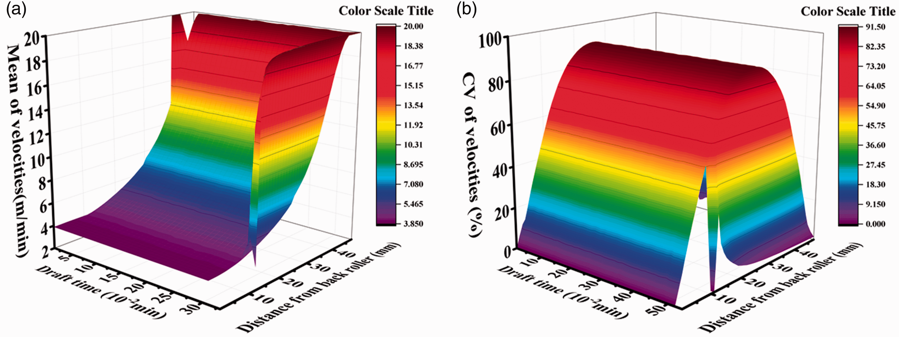

In the roller drafting process, the sliver moves forward due to the velocity disparity between the fast speed of the front roller and the slower speed of the back roller. Accordingly, the velocities of fibers exert dynamic variance with the distance from the back roller. Figure 11 shows the profile of the mean and CV of fiber velocities in the drafting zone with various drafting conditions. It can be seen from the profiles of the mean variance that it shows a growing trend toward the front roller and the skewness of mean velocity growth becomes larger on approaching the front roller. It can be concluded that fibers in the sliver are continuously accelerated in the draft zone as the sliver moved forward, and the number of accelerated fibers increases on approaching the nip line of the front roller. The CV of fiber velocities increases from the back roller to a maximum in the middle of the drafting zone, then quickly goes down to 0 near the nip line of the front roller. This shows that fiber velocities fluctuate significantly in the middle of the drafting zone.

Figure 11.

The simulated mean and CV of fiber velocities in the sliver in the drafting zone for various drafting conditions: (a) draft ratio; (b) gauge length; (c) delivery speed; (d) input sliver linear density.

Figure 12.

The simulated mean and CV of fiber velocities in the sliver in the drafting zone for various distributions of fiber accelerated points.

Besides, it can be seen from Figure 11(a) that the mean velocity has a declining trend as the draft ratio increases. By contrast, the CV of fiber velocities increases as the draft ratio grows. In other words, the simulative results show that the fiber motion in the draft zone can be more impressionable as the draft ratio increases while the velocity CV% increases.

Regarding gauge length (Figure 11(b)), the slope of the mean velocity profile at the nip point of the front roller becomes smaller as the gauge length increases. The maximum of velocity CV is same in the middle of the drafting zone. Due to the growth of gauge length, the CV value near the back roller becomes lower, while the CV value close to the front roller increases as the gauge length grows.

In contrast, the CV of fiber velocities barely changes as the delivery speed increases, as shown in Figure 11(c). It can be interpreted that the fiber motion fluctuation in the drafting zone will be free from the delivery speed, while the other drafting parameters remain constant. However, the mean velocity profile shows that the curves have different shapes to a great extent. The slope of the velocity profile grows as the delivery speed increases near the nip line of the front roller. It can be expected that the sliver can have a greater possibility of behavior disturbance near the front roller at a high delivery speed.

In addition, the mean and CV of fiber velocities during the drafting process are almost in accordance, despite the diverse input sliver linear density, as depicted in Figure 11(d), which indicates that the input sliver linear density does not have a significant effect on sliver dynamics.

Similar to the simulated attenuation curves of sliver linear density, as shown in Figure 12, the simulated mean and CV of fiber velocities in the sliver in the drafting zone with ideal identical accelerated points are drastically different from the simulated ones with different accelerated points. Meanwhile, the simulated mean and CV of fiber velocities with the accelerated-point distributions of Parabolic, Weibull and log-normal obviously differ from each other, which is caused by the disparate rates of divergence for these three acceleration distributions, as shown in Figure 3. What is more, the simulations of mean and CV for fiber velocities with the actual and log-normal distributions of accelerated positions have a slight distinction from the result of the similar distribution in Figure 3.

Considering the above results, the fiber motion in the drafting process could be analyzed quantificationally and specifically by the proposed drafting model. It turns out that the mean velocities of fiber in the drafting zone are influenced by the draft ratio, gauge length and delivery speed, while the CV of fiber velocities are affected by the draft ratio, gauge length and input sliver linear density. Besides, during the drafting simulation, the distribution pattern of fiber accelerated points has an obvious contribution to the simulated mean and CV of fiber velocities in the sliver in the drafting zone.

Conclusion

This research simulated sliver motion during the drafting process based on the model of fiber arrangement. In this simulation, fiber arrangement in the sliver before drafting was firstly supplied, then the drafting process can be originated from the high-velocity motion of the first accelerated fiber and end in the high-velocity motion of the last accelerated fiber. The fiber distribution in the drafting zone was simulated from the fiber arrangement in the real time. Meanwhile, the sliver dynamics during the drafting process can be analyzed by the attenuation of sliver density and the fiber velocities in the drafting area.

The developed drafting model accomplished the quantization goal of the drafting process, which will provide improvement in understanding of the drafting theory. Specifically, the simulation results of the model revealed that the simulated attenuation curves of sliver linear density were compatible with the experimental results. Furthermore, it could be inferred that the attenuation process of the sliver in the drafting area was influenced greatly by the draft ratio, gauge length, input sliver linear density and distribution pattern of fiber accelerated points, but barely influenced by the delivery speed. In addition, fibers with different characters in the zone between the nip point of the front and back rollers could be explicitly and precisely simulated by fiber arrangement in real time. Last but not least, it could be drawn from the calculated simulation results that the draft ratio, gauge length and delivery speed played important roles in the mean velocity of fiber in the drafting zone, while the CV of fiber velocities was significantly related to the draft ratio, gauge length and input sliver linear density. Besides, the distribution pattern of fiber accelerated points distinctly works on the simulated mean and CV of fiber velocities in the sliver in the drafting zone. More importantly, the simulations of the fiber distribution and the velocity of fibers in the drafting zone were realized, which are currently still difficult to be intuitively tested by the actual used methods. Therefore, the fiber motion in the drafting process could be specifically understood by the obtained fiber distribution and the mean and CV of fiber velocities from the drafting model. The model could be of significant guidance in choosing the appropriate drafting parameters in the practical manufacture process based on the simulated fiber motion.

Footnotes

Declaration of conflicting interests

The authors declared no potential conflicts of interest with respect to the research, authorship and/or publication of this article.

Funding

The authors disclosed receipt of the following financial support for the research, authorship, and/or publication of this article: This work was supported by National Natural Science Foundation of China (No.51773034).

References

Rao

. A mathematical model for the ideal sliver and its applications to the theory of roller drafting. J Text Inst 1961; 52: 571–601.

Taylor

. The motion of floating fibres during drafting of worsted slivers. J Text Inst 1955; 46: 284–294.

Taylor

. The velocity of floating fibres during drafting of worsted slivers. J Text Inst 1959; 50: 233–236.

Weber

Wulfhorst

. Fiber motion in roller drafting. Text Res J 1997; 67: 10–13.

Yao

Chen

. Modeling and simulating the motion of floating fibers during drafting. J Donghua Univ 2006; 32: 1–5.

Yan

. The influence of fiber length distribution on the accelerated points in drafting: a new perspective on drafting process. Fiber Polym 2009; 10: 217–220.

Lin

Oxenham

. Effect of accelerated point distribution on sliver irregularity. Part I: characterization of accelerated point distribution. J Text Inst 2012; 103: 549–557.

Lin

Oxenham

. Effect of accelerated point distribution on sliver irregularity. Part II: optimization of draft settings in two-zone roller drafting system. J Text Inst 2012; 103: 558–564.

Johnson

NAG

. A computer simulation of drafting. J Text Inst 2008; 72: 69–79.

10.

Huh

Kim

. Modeling the dynamic behavior of the fiber bundle in a roll-drafting process. Text Res J 2004; 74: 872–878.

11.

Huh

Kim

. Effects of material parameters and process conditions on the roll-drafting dynamics. Fiber Polym 2006; 7: 424–431.

12.

Huh

Kim

. Occurrence of a singular point in a bundle flow system and the sensitivity of the bundle thickness to perturbations in a steady state draft process. Text Res J 2008; 78: 843–855.

13.

Kim

Cherif

Huh

. Numerical analysis of fiber fleece behavior in roller drafting in a transient state. Text Res J 2008; 78: 796–805.

14.

Kim

Huh

Suh

M W

. A method to generate autocorrelated stochastic signals based on the random phase spectrum. J Text Inst 2010; 101: 471–479.

15.

Kim

Cherif

Huh

. Dynamic stability and bifurcation in a bundle flow. Nonlin Anal -Real World Appl 2011; 12: 343–352.

16.

Kim

Suh

Huh

. Analysis of sliver thickness variation from process perturbations in roller drafting. J Text Inst 2012; 103: 1055–1062.

17.

Cherkassky

. Discrete-event simulation model of roll-drafting process. J Text Inst 2011; 102: 1044–1058.

18.

Cherkassky

. Neural network meta-model of fibrous materials based on discrete-event simulation. Part 1: discrete-event simulation model of one-dimensional fibrous material. J Text Inst 2011; 102: 442–454.

19.

Wang

. Study on the fiber distribution in a drafting zone. J Text Inst 2017; 108: 1057–1064.

20.

Jiang

Kuang

, et al. Simulation on fiber random arrangement in the yarn. J Text Inst 2014; 105: 1312–1318.

21.

Zhang

Jiang

, et al. Mathematical modeling of ideal yarn based on Poisson process and the analysis of yarn unevenness. Math Pract Theor 2017; 47: 229–234. .

22.

Spencer-Smith

Todd

HAC

. A time series met with in textile research. Wiley R Stat Soc 1941; 7: 131–145.

23.

Brown

. Statistics for the number of fiber ends in a segment of a random assembly of aligned fibers. Text Res J 1985; 55: 206–210.

24.

Mupfudze KD, Cao Q, Shen Y, et al. Fiber motion and the accelerated point distribution in roller drafting. Text Res J. Epub ahead of print 16 April 2018. DOI: 004051751876715.