Modeling and realization for appearance visualization of Textronic laces

Abstract

A computing approach based on the warp-knitted fabric structure was presented in this paper to visualize Textronic laces by taking a fall-plate lapping in one course as a targeted unit. Its geometric description was firstly presented on both the projection plane and normal plane of structure depth. Based on this and an improved Blinn–Phong reflection model, illuminative interaction along the yarn width and lapping length was separately studied and then overlaid with empirical weight coefficients to fit a function to solve fall-plate lapping facial illumination. Because the displayed facial feature was illustrated by distinguishing pixels on screen, the continuous solved function was discretized into average grids and each grid was integrating to obtain segmental appearance variation. The variation was then mapped from a Cartesian coordinate to a screen coordinate of pixels to be displayed, while the hidden lapping was eliminated according to the depth-buffer algorithm.

Keywords

warp knitting fabric simulation illumination model geometry modeling hidden-surface elimination

Textronic lace, manufactured on a multi-bar warp knitting machine with a fall-plate mechanism, is comprised of ground jacquard net, major fall-plate patterns and associated inlay patterns. Distinguished from Jacquardtronic laces, Textronic lace highlights the advantage of stereopsis impression with fall-plate structures. Because of the complete difference between lace drafting and fabric appearance, a great challenge for the designer is how to predict and visualize the lace appearance and make revisions during the design process to reduce sample-making. A computer-aided simulation module can possibly make this happen. Studies on fabric visualization began and have been developed in both the areas of computer graphics and textile engineering since the 1930s, when the first model was proposed by Pierce.¹ The present simulation approaches are basically categorized into image-based and geometry-based methods. The image-based methods, such as texture mapping^2,3 and bump mapping,⁴ fundamentally emphasize the distinction of pixel color intensities using a simplified lighting model and texture image, rather than solving the geometric positions of surfaces. Özdemir and Başer^5,6 presented a photograph-based model to simulate the surface appearance of plain woven fabrics by obtaining real yarn images and resizing them to be mapped to flattened and crimped structures based on raster graphics (Figure 1(a)). Li et al.⁷ visualized wrapped warp-knitted laces by concluding algorithms of color intensities based on real yarn photographs (Figure 1(b)). These image-based methods greatly reduced computation time because there is no need to render spatial meshes and curves. However, they neglected the effect of structural geometry on fabric reflection properties. Lu and Jiang⁸ transformed real yarn textures to a two-dimensional (2D) flat-knitted loop model with a shading coefficient due to the consideration of geometric interlacing and depth information (Figure 1(c)). It realized realistic appearance simulation but was limited to regular flat-knitted structures because all texture and loop models were allocated from a prepared database.

Figure 1.

Image-based simulation of (a) woven fabric,^5,6 (b) warp-knitted lace⁷ and (c) flat-knitted fabric.⁸

Some scholars proposed geometry-based methods by using an illumination model and generating textile structural geometries. Yuksel et al.⁹ studied the visualization of flat-knitted cloth (Figure 2(a)) by using stitch-mesh polygons rather than single loop units. Kyosev¹⁰ presented how to use the finite element method to generate three-dimensional (3D) geometry of yarns and knitted structures with TexMind Software (Figure 2(b)), including the twisted yarn geometry of numerous filaments. Similarly, Lin et al.¹¹ provided a 3D description of woven fabrics (Figure 2(c)) in TexGen, defining a section curve and sweeping it along the yarn path to form an individual yarn solid, and then bending the warp and weft yarns to illustrate 3D interlacement. These 3D approaches showed more detailed structure information, which conversely increased computation time and lowered simulation efficiency. Shang et al.¹² viewed interlaced yarns as cylinders and then built an improved 2D illumination model to generate 3D visual effect (Figure 2(d)) with less computation. Apart from these analytical models, commercial computing programs have also been made available for use throughout the textile industry. The latest version of ProCad® has realized 3D modeling and simulation of Textronic laces, but revealed a defect in the frame rate, namely a delayed rendering.

Figure 2.

Geometry-based simulation of (a) a flat-knitted structure based on stitch meshes,⁹ (b) a circular knitted structure,¹⁰ (c) woven fabric with a three-dimensional model,¹¹ and (d) woven fabric with a two-dimensional model.¹²

The computer visualization of inlay pattern structures and ground Jacquard structures has been realized.^7,13 The objective of this research is to develop a real-time and realistic approach for visualizing fall-plate pattern appearance after pattern drafting and yarn property defining. So, we focused on what illumination appearance would be generated under the fall-plate structure geometry and lighting model. To achieve this goal, study needs to be done in terms of the following:

representing fall-plate geometric structures based on the chain notation chart;

modeling and solving facial illumination interaction on fall-plate lapping structures;

displaying appearance variation by transferring the result from Cartesian coordinates to pixel coordinates;

detecting the visible and hidden surfaces.

Basic assumptions

Undeformed yarn section

In a fabric simulation model, a yarn is generally described as a non-rigid solid volume with an approximated circle or elliptical cross-section. When it is looped to form fall-plate structures, tiny deformations happen that slightly change the reflection performance on the positioned surfaces, resulting in massive computation of illumination intensity. So, the cross-section of fall-plate yarns is assumed as undeformed. In addition, compared with large pattern sizes in meters, the geometric details of yarns in millimeters are rarely observed when illustrated at their original size. So, a yarn is assumed as a single volume regardless of twist and filaments in order to reduce computation.

Underlapping fall-plate structure

Simulation results of Textronic laces concentrate on the overall visualization of fall-plate patterns rather than individual fall-plate loops. Fall-plate overlaps, in the original simulation size, are almost invisible because of coverage by part of the underlaps when vertically observed. Based on that, fall-plate structures are simplified as intersected underlaps on the simulation plane.

Infinite light source

The simulator developed in this paper aims to show a visualized appearance of Textronic laces in natural sunlight, which is so far away from the simulation scene that the light source is assumed to be infinite in order to neglect its exact location. Lighting paths from the source to any point on simulated object are nearly unchanged, which means a lighting vector can be used for representing all paths of incident light and the intensity remains constant on the simulation scene.¹⁴ Therefore, the infinite light source is defined with a single RGB (r_s, g_s, b_s), which is mostly white and a vector S vertical to the simulation plane (Figure 3). Usually an observation vector O is defined as parallel to the light source vector S.

Figure 3.

Illustration of the light source and viewpoint.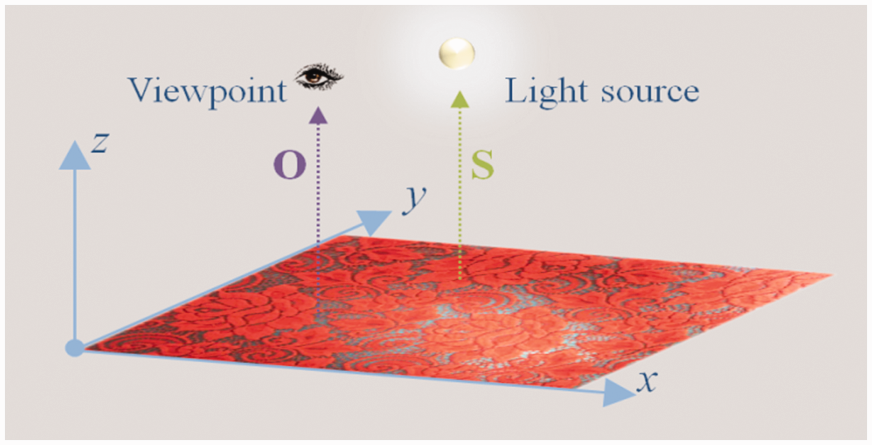

Local lighting model

To calculate the light intensity at projection points on the simulation plane, a simplified local lighting model is preferred in this paper in order to reduce computation by excluding ambient light reflected from neighborhood objects.¹⁵ Incident light reaches an observer to form a visualized impression because of diffuse and specular reflection from the surface of an object. Diffuse reflection contributes much less since the observation is parallel to the incident vector. The diffuse reflection coefficient is defined as a constant k_d, based on Lambert's cosine law,¹⁶ and all surfaces have equal diffuse reflection intensity I_d. A modified Blinn–Phong specular reflection model¹⁷ (Figure 4) is used to compute specular reflection I_s according to Equation (1). The light intensity captured by the observer is solved by Equation (2). In these equations, k_s and n_s are respectively used as the coefficient and exponent of specular reflection, which are related to the facial smoothness of the yarn. I_l is the intensity of incident light. O, R and S are the unit vectors of observation, reflection and the light source, respectively. N is the unit normal vector at a given point. No specular reflection can reach the observer when the angle between the observation (the incident direction) and the reflection direction is equal or greater than $\frac{π}{2}$ . Appearance variation is basically related to specular reflection performance, which is highlighted below

I_{s} = \begin{matrix} {\begin{matrix} k_{s} I_{l} {(O \cdot R)}^{n_{s}}, O \cdot R > 0 \\ 0, O \cdot R \leq 0 \end{matrix} \end{matrix}

(1)

I = I_{d} + I_{s} = k_{d} I_{l} + k_{s} I_{l} (O \cdot R)^{n_{s}}

(2)

Figure 4.

Modified Blinn–Phong specular reflection model.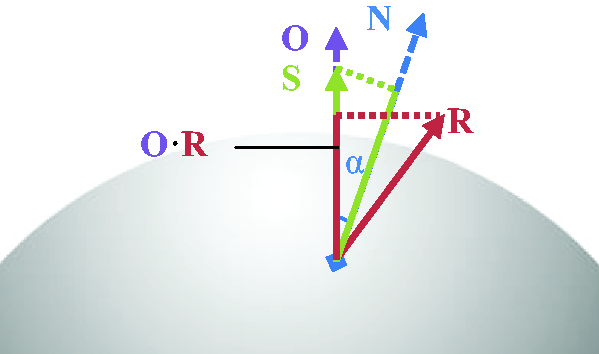

Modeling process

Representation of fall-plate pattern structures

Most lace patterning computer-aided design (CAD) programs prefer a generic data-based technique for representing knitted patterns with zero-positions and lapping configuration files. This technique was initially designed for manufacturing rather than computer-aided visualization, so it is firstly interpreted into structural geometries and then simulated by computer graphics for visual simulation. Zero-positions refer to the firstly overlapped wales of each pattern bar on the first course. The lapping configuration decides the lapping direction and distance when underlapping and overlapping on each course. If the zero-position of one fall-plate pattern bar is referred to as p, the lapping data on courses No. i and No. i + 1 are defined as m_i, (m_i + r_i), m_i+1, and (m_i+1 + r_i + 1), where m_i and m_i+1 represent the start chain numbers, while r_i and r_i + 1 are the shifting distances when overlapping. The overlapped wales denoted as W_i and W_i + 1 on these two courses are solved by the following equations

W_{i} = max {p + m_{i}, p + m_{i} + r_{i}}

(3)

W_{i + 1} = max {p + m_{i + 1}, p + m_{i + 1} + r_{i + 1}}

(4)

If r_i > 0, it means that the stitch is overlapped from right to left across r_i wales; if r_i < 0, the stitch is overlapped from left to right; if r_i = 0, it is an inlay structure with no overlapping. Whether the stitch is open or closed is relied on the product q represented by Equation (5)

q = [(m_{i} + r_{i}) - m_{i}] \times [{m_{i +}}_{1} - (m_{i} + r_{i})]

(5)

If q > 0, it is an open stitch (Figures 5(b) and (c)), but if q < 0, it is a closed stitch (Figures 5(a) and (d)). The final loop geometry is also related to the overlapping direction of the ground pillars. Four types of fall-plate lapping diagrams and corresponding loops are shown in Figure 5. The first two types whose fall-plate and ground pillar are overlapping in the same direction are mostly used in Jacquard curtain fabrics. The last two types with opposite directions are mainly for multi-bar Textronic laces. In particular, the last diagram shows a superior stereopsis impression, so it is mostly preferred and taken in this paper as a basic unit example to be geometrically modeled for computer-aided visualization.

Figure 5.

Lapping diagrams (a), (c), (e), (g) and their corresponding loop structures (b), (d), (f), (h), respectively.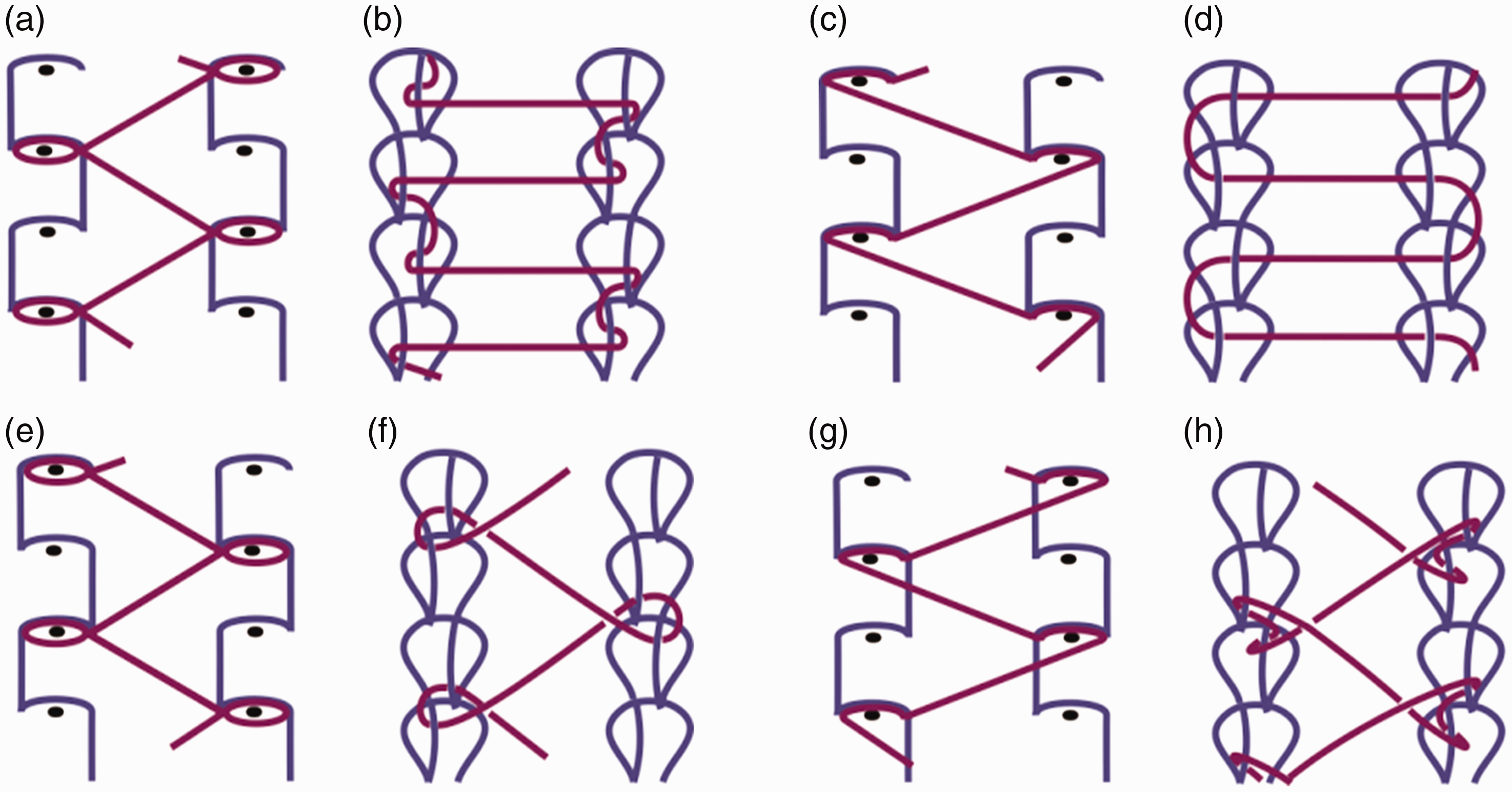

The structure shown in Figure 5(h) is a theoretical one based on the knitting process. However, when it is knitted into laces, elasticity from pillar underlaps is loaded for restriction, resulting in deformation (Figures 6(a) and (b)). In particular, it looks more like a pillar structure when it is kept stitching on one wale (Figures 6(c) and (d)). This is chosen where fall-plate yarns need to be hidden under other patterned lapping or designed as pattern contours.

Figure 6.

Fall-plate stitches with deformation under yarn tension: (a) lapping across wales and (b) the corresponding deformed geometry from the side view; (c) lapping on one wale and (d) the deformed geometry from the side view.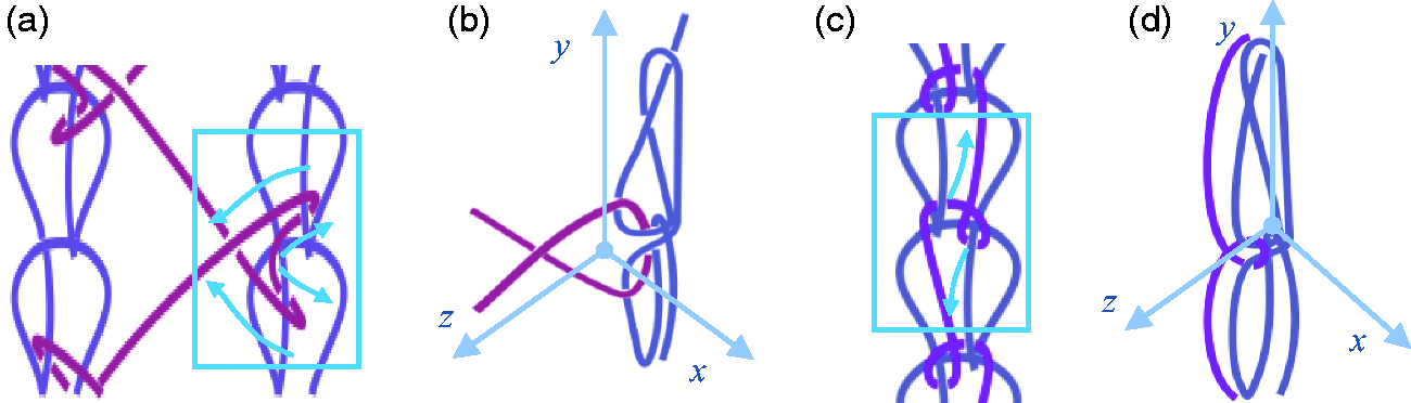

Solving the illumination interaction

To simulate illumination interaction on the appearance of Textronic laces, projected geometries need to be built and then a solution for varying facial lightness should be solved. An approach is used here in which fall-plate pattern structures are firstly projected on the simulation plane as continuously interlaced segments, as shown in Figure 7. The x-axis represents the width of the lace pattern and the y-axis represents the length, namely the knitting direction. The z-axis is parallel to the observation vector and light source vector. The light intensity of each point on the projection plane x–y is equal to I₁, which is obtained by the product of k_s and I_l. Variable n is the number of wales underlapping across, obtained by Equation (6); W_pc and C_pc are the wale density and course density in 1 cm; l is the length of the projected underlap in mm, calculated by Equation (7); d refers to the diameter of fall-plate yarns in mm; and θ is the angle between the underlap and the x-axis. Generally, Textronic laces are manufactured using multi-bar Raschel machines with a gauge of E24 or E28, making W_pc vary from 9 to11 wales/cm and C_pc from 35 to 40 courses/cm. When n ≥ 3, θ is approximately less than 6°, meaning that it is small enough to make l approximate to $n \times \frac{10}{W_{pc}}$ .

Figure 7.

The simplified projection of fall-plate lapping structures.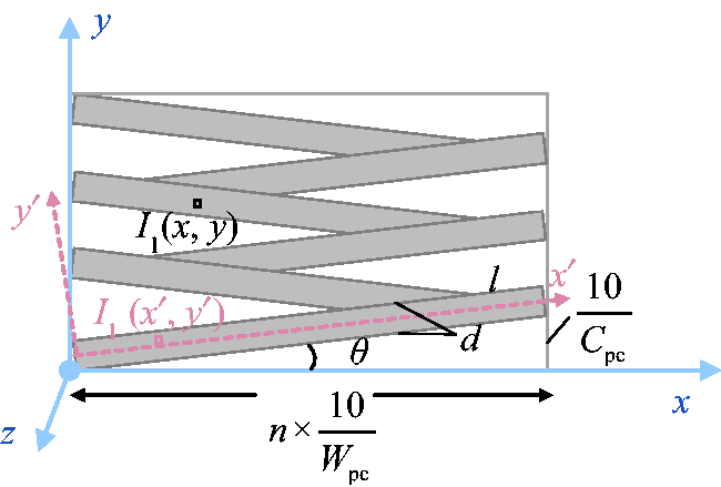

Although the fall-plate course is assumed to be a rectangle segment on the projection plane, it is in fact a column, which means that when it is being lighted, along the yarn diameter the light intensity varies according to a specific function f (y′). Here an associated coordinate of x′–y′ (Figure 8) is added and transformation from x–y to x′–y′ is calculated by Equations (8) and (9)

n = | {m_{i +}}_{1} - (m_{i} + r_{i}) |

(6)

l = \sqrt{(n \times \frac{10}{W_{pc}}) 2 + (\frac{10}{C_{pc}}) 2}, n \geq 1

(7)

x' = x cos θ + y sin θ

(8)

y' = y cos θ - x sin θ

(9)

Figure 8.

Coordinate system transformation from x–y to x′–y′.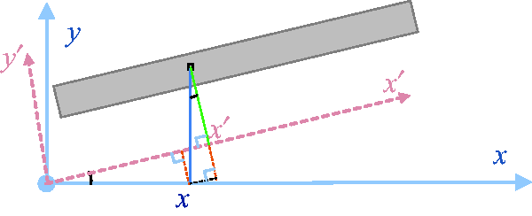

Because they feature stereopsis, fall-plate yarns mostly have a shining appearance; their reflection performance along the yarn diameter is presented in Figure 9 based on the previous research carried out by Li et al.⁷. y′_L and y′_R represent the coordinates of two edge points. When computed, the continuous function f (y′) is discretized into a set of equal histograms. The height of the histogram solved by Equation (10) represents the average light intensity of interval y′₁y′₂. c is a coefficient of the inflection point on the illumination curve. This model merely considers illumination variation along the yarn diameter and ignores the variation caused by interlaced deformation

\begin{matrix} I_{2} (y'_{1}, y'_{2}) = {\begin{matrix} I_{1}, cd \leq y' \leq (1 - c) d \\ \frac{1}{y'_{2} - y'_{1}} \int_{y'_{1}}^{y'_{2}} I_{2} (y') d y', 0 \leq y' < cd and (1 - c) d < y' \leq d \end{matrix} \end{matrix}

(10)

Figure 9.

Reflection performance of the fall-plate yarn along the cylindrical periphery.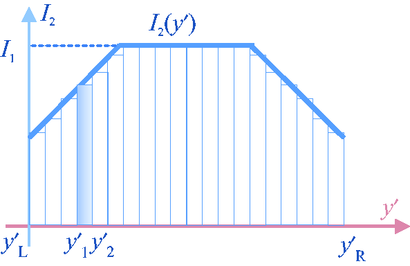

Except for light variation along the yarn diameter, the primary feature of fall-plate structures lies in the lighting difference in the lapping length, which is decided by the structural geometry. A simplified model is proposed (Figure 10) based on the geometry shown in Figure 6(b). It defines the lapping path of one course as a basic unit instead of one single yarn. h symbolizes the maximum height of the fall-plate structure in the z-axis. Based on the loop forming principle, h is approximate to the width of one loop, which is related to the machine gauge E.¹⁸ Angle φ indicates tangent slope of a point on the underlap curve against the x′-axis and can be determined by a derivation of the curve function at that point. The function of underlap is related to n, which theoretically varies from 1 to $\frac{E}{2}$ , and with the increase of n it is gradually close to a linear one. For a lace pattern with massive lapping movement, calculating φ usually requires excessive computation. Because of this, the illumination curve of a fall-plate underlap is simplified as a linear segment, shown in Figure 11. When computed, the continuous illumination curve is discretized to represent variation. Along the underlapping direction, the intensity I₃ (x′) is solved by Equation (11)

I_{3} (x'_{1}, x'_{2}) = \frac{1}{x'_{2} - x'_{1}} \times \int_{x'_{1}}^{x'_{2}} I_{3} (x') d x', 0 \leq x' \leq l

(11)

Figure 10.

Deformed geometry of the fall-plate structure.

Figure 11.

Average reflection intensity along the yarn length.

For a special fall-plate structure that is linearly lapped, based on its geometry in the z-axis (Figure 6(d)) its illumination curve with discretized variation is as illustrated in Figure 12. It can be seen that the visible underlap curve approximates to a half ellipse. The height of the hidden overlap Δh is referred as the sum of the fall-plate yarn diameter and is twice the diameter of pillar yarn. Except for the number of underlapped wales, the length l′ is also related to the number of courses between two continuous looped points. l′ is calculated by Equation (12), where n′ represent the number of underlapped courses

l' = 10 \sqrt{(\frac{n}{W_{pc}}) 2 + (\frac{n'}{C_{pc}}) 2}

(12)

Figure 12.

Deformed geometry in the z-axis when linearly lapped.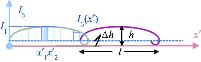

The above illumination functions when solved can be used for simulating light variation along the yarn diameter and yarn length. Each individual solving cannot achieve realistic appearance visualization of fall-plate patterned structures unless these two parts are overlaid together. As a result, the final illumination function I (x′, y′) of overlaid specular intensity is solved by Equation (13), where q₁ and q₂ are the weight coefficients of intensity I₂ (y′) and I₃ (x′). The average intensity of each unit area on projected lapping is presented by the product of dx′ and dy′. Figure 13 shows the simulated results by varying values of q₁ and q₂. It is easily noticed that when q₁ < 0.4, a sharp attenuation of light intensity happens along the yarn diameter, showing an unnatural yarn geometry. When q₁ > 0.5, a sudden change of light intensity occurs at the intersection point of the segmental underlap and curved overlap, which results in unreal simulation of the fall-plate lapping characteristic. Although the change at the intersection point when q₁ = 0.5 is not so obvious, it is still not as realistic as the result when q₁ = 0.4. Therefore, q₁ and q₂ are finally defined as 0.4 and 0.6, respectively.

Figure 13.

Simulated results with various values of q₁ and q₂: (a) q₁ = 0.1, q₂ = 0.9; (b) q₁ = 0.2, q₂ = 0.8; (c) q₁ = 0.3, q₂ = 0.7; (d) q₁ = 0.4, q₂ = 0.6; (e) q₁ = 0.5, q₂ = 0.5; (f) q₁ = 0.6, q₂ = 0.4, (g) q₁ = 0.7, q₂ = 0.3; (h) q₁ = 0.8, q₂ = 0.2; and (i) q₁ = 0.9, q₂ = 0.1.

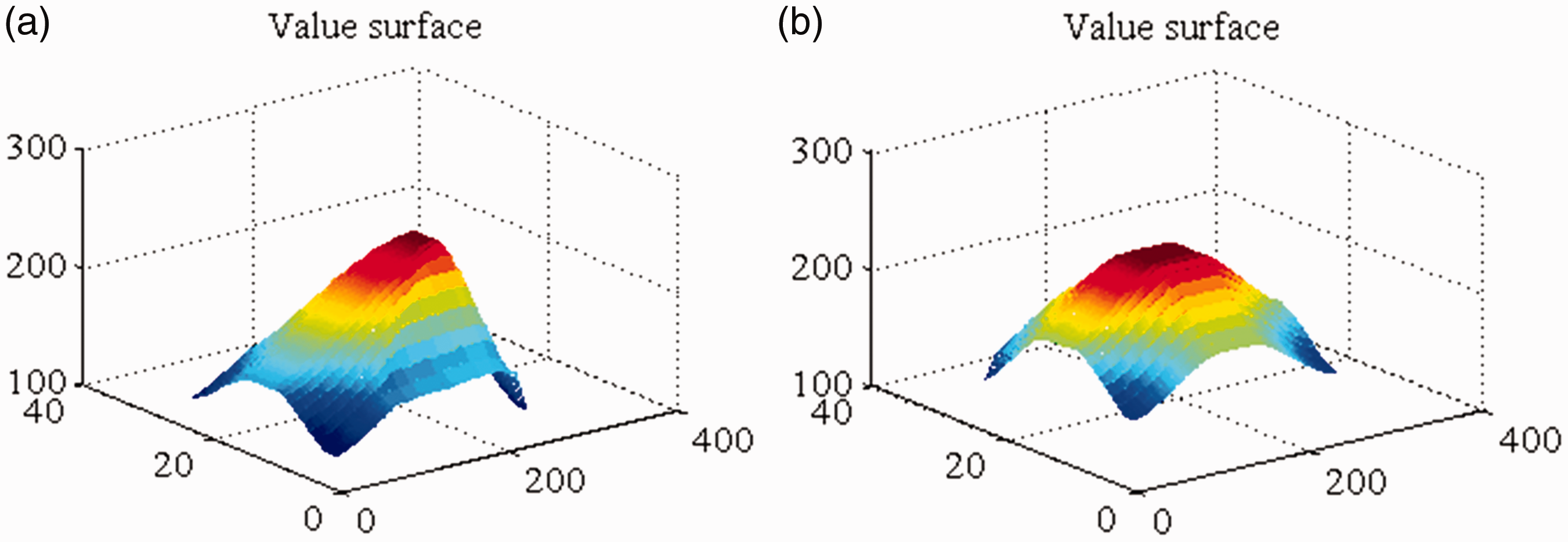
Normally, facial light variation of fall-plate structures is generated by four steps: simplifying lapping structures as interlaced segments with even intensity I₁; solving I₂(y′) along the yarn diameter; solving I₃(x′) along the lapping length; and summing individual I₂(y′) and I₃(x′) for compound simulation. Simulated yarn effects under the four steps are shown in Figure 14. By comparing, it is easy to conclude that the final two compound effects show a realistically simulated appearance. The value surfaces of the last two compound effects in Hue, Saturation and Value (HSV) mode are shown in Figure 15, and have good consistency with the simplified geometries of fall-plate lapping structures

I (x', y') = q_{1} \times I_{2} (y') + q_{2} \times I_{3} (x') + I_{d}

(13)

Figure 14.

Simulation results of illumination variation obtained by (a) even density I₁; (b) I₂; (c) I₃ underlapped across wales; (d) I₃underlapped on one wale; (e) I underlapped across wales; and (f) I underlapped on one wale.

Figure 15.

Value surfaces with light intensity I on simulated fall-plate structures that are (a) underlapped across wales and (b) underlapped on one wale.

Simulation realization

After illumination variation is solved, it needs to be displayed on a screen of pixels as simulation results. Because of numerous guided bars lapping simultaneously, the detection of invisible segments is required where yarns are overlaid. The following part presents a mapping theory from the Cartesian coordinate to a screen coordinate and generates an algorithm of hidden-surface elimination.¹⁷

Coordinate mapping

Visualizing simulation results on a display screen is used to define the color attributes of each lapped pixel. The light intensity obtained by fitted equations discretized into average values of uniform meshes,¹² which is explained as below.

(1) Mark the left top and right bottom coordinates of the pattern geometry and obtain the corresponding pixels on the simulated plane, respectively referred to as g(x_L, y_L), g(x_R, y_R), p(X_L, Y_L), p(X_R, Y_R).

(2) Calculate the average illumination intensity of a unit area in the Cartesian coordinate according to Equation (14)

I (d x, d y) = \int I (x, y) d x d y

(14)

(3) Solve the area S of one pixel based on Equation (15)

S_{pixel} = \frac{(x_{R} - x_{L}) \times (y_{R} - y_{L})}{(X_{R} - X_{L} + 1) \times (Y_{R} - Y_{L} + 1)}

(15)

(4) Obtain the final illumination value I_pixel of one pixel by Equation (16)

I_{pixel} = S_{pixel} \times I (dx, dy) + I_{d}

(16)

In particular, it is possible that pixels around the pattern periphery are not fully filled, which means that S is smaller than S_pixel. Under this assumption, the pixel is still completely designed but with a smaller intensity than I_pixel.

Hidden-surface elimination

Similar to Rascheltronic laces, when rendering a surface of fall-plate patterns it is likely that two or more points are mapped to the same pixel where lapping lines are overlaid. To address this issue, an improved depth-buffer approach, which is also called the z-buffer algorithm,^7,19 is used (shown in Figure 16) to erase hidden surfaces. Each point of the projected patterns is defined with two characteristics, the color value and the depth value, which are memorized in two separate caches. The depth value includes both a pattern bar number and a course sequence. Lapping movements of each pattern bar are drawn on a separate plane P_j, where j is the plane depth, namely the guided bar number. All of the planes are sequenced by their depth and the first one is positioned closest to the simulation plane. Lapping segments of the same pattern bar on one plane are sequenced by the course number t according to the knitting direction. The depth value of pixels on the simulation plane is firstly initialized as j₀ (the maximum bar number), and the color is defined the same as the simulation background. Although the HSV space can intuitively express the brightness, color and vividness of the color, which facilitates the contrast between colors and perception by eye, it cannot directly represent colors on the display. RGB space is a popular mode to store, represent and display colors on illuminators. So, a transforming algorithm⁷ connects these two modes well. The color of the simulation background is designed as RGB (r₀, g₀, b₀). Then the pattern planes are separately generated based on parameters of the knitting direction, zero-position, lapping configuration and the solved illumination variation. When two segments on one plane are overlaid, the visible sequence is related to the fall-plate structure type and the course number. For open stitches, the course with a smaller t is visible (as in Figure 16(a)), but for closed stitches a course with a greater t is rendered (as Figure 16(b)). Afterwards, all planes are consequently scanned from pixel (X_R, Y_R) to (X_L, Y_L) and if j < j₀, the color value (r₀, g₀, b₀) is replaced by (r_j, g_j, b_j). When two points on different planes are mapped to the same pixel, the point with a smaller depth value is visible. After all planes are scanned, pixels on the display screen are assigned with new attributes and finally show simulated fall-plate lace patterns.

Figure 16.

Hidden-surface elimination model: (a) open fall-plate stitch model; and (b) closed fall-plate stitch model.

Simulation results and discussion

With the visualization approach proposed above, an appearance simulator for Textronic laces is programmed by Visual C+ + in a Windows 7 system, Intel Core i5-7500 CPU and 8 GB RAM, based on a lace pattern drafting CAD software. The simulator is developed a Textronic pattern, which is designed and taken as an example to test this simulator, formed by one pillar ground guided bar, two split inlay jacquard bars, seven inlay pattern bars and 14 fall-plate pattern bars. Before simulation, the basic parameters are designed, including the pattern density, simulation resolution, yarn fineness, yarn color and yarn brightness (shown in Figure 17). The yarn cross-section here is defined as a circle shape. For this simulated example, it has 46 wales and 180 courses with an area density of 11 wales and 36 courses in 1 cm². The simulation resolution determines the generating speed and quality of the simulated results. Considering the huge pattern and simulating efficiency of lace, the resolution here is designed as 850 pixels per inch. The configuration of the yarns in each guided bar is shown in Table 1. The simulation results generated and their corresponding enlarged results are respectively shown in Figure 18.

Figure 17.

Yarn parameter design.

Figure 18.

Simulation results formed by (a) the first step I₁, (b) the secnd step I₂, (c) the third step I₃ and (d) the fourth step I.

Table 1.

Yarn configuration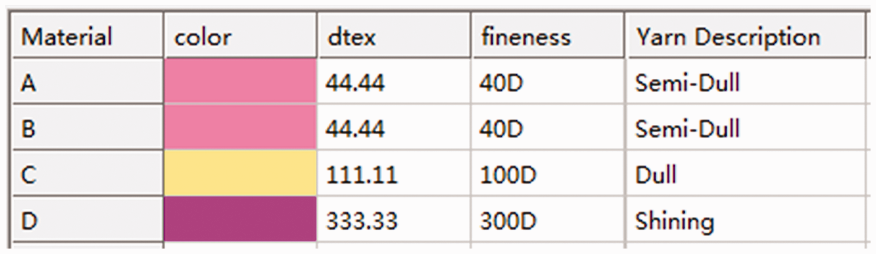

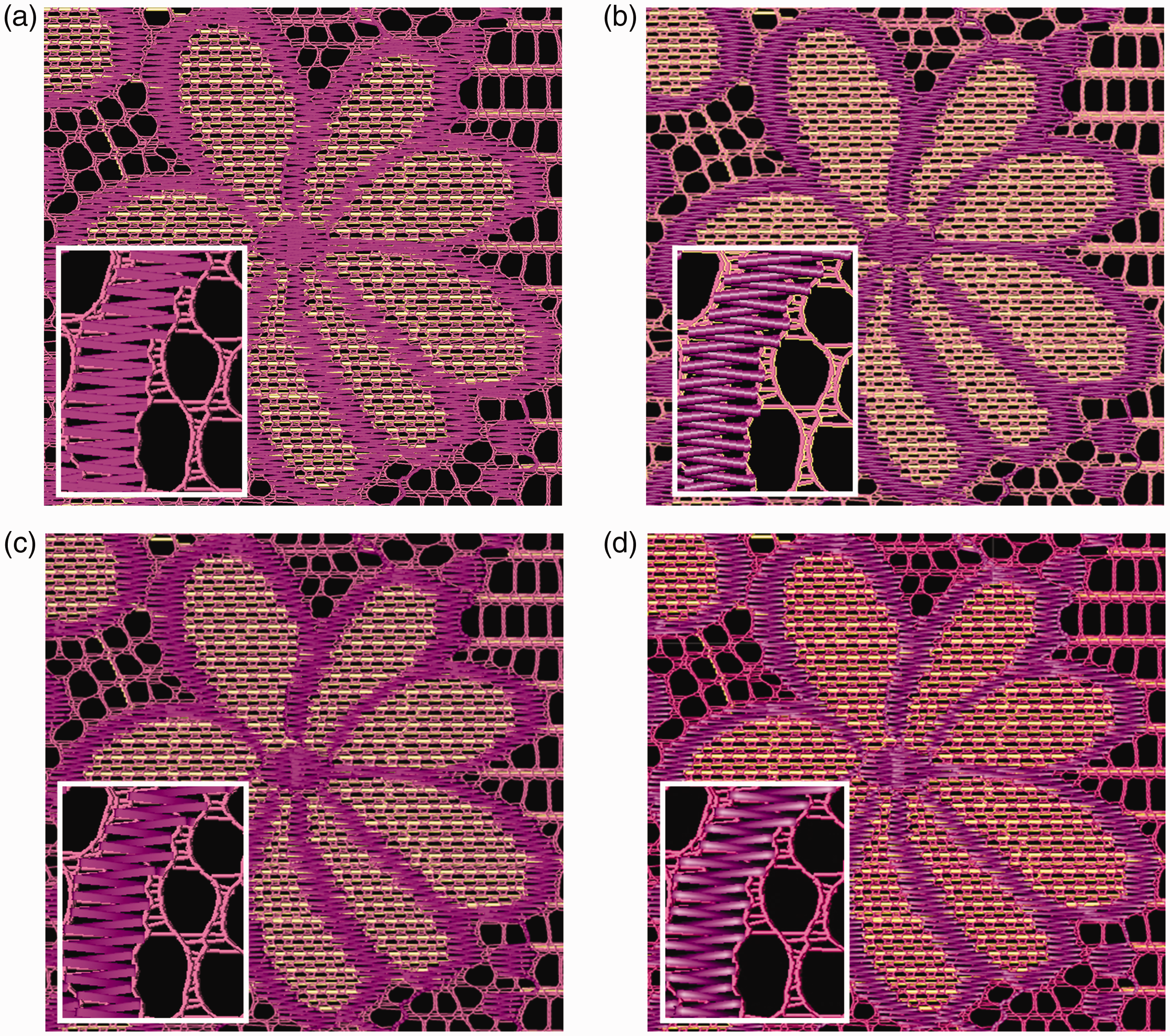
Guided bars	Yarn fineness	Yarn color	Yarn brightness
Ground pillars	44 dtex	RGB(255,128,192)	Semi-dull
Inlay jacquard	44 dtex	RGB(255,128,192)	Semi-dull
Inlay patterns	110 dtex	RGB(255,255,128)	Dull
Fall-plate patterns	330 dtex	RGB(240,0,240)	Shining

By comparing these four figures, it is shown that the first simulation result of fall-plate patterns is relatively plain because it does not show illumination variation either along the yarn diameter or the lapping length. The second result makes an improvement by varying the light effect along the yarn diameter but impossibly illustrates the features of the fall-plate structure. The third one reveals appearance changes along the fall-plate lapping length to show structural features, but lapping segments appear as flat tapes without the features of yarn cylinders. By combining the second and third effects together, the fourth result improves the appearance visualization both in yarn impression and fall-plate geometry. It realizes a relatively realistic effect. The simulation time of each result was tested 10 times to avoid accidental errors. Figure 19 shows the tested results and, from a comparison, we know that the simulation time of compound lighting is about 10 milliseconds longer than the single lighting obtained by the first step. This means a lace pattern repeat of more than 50,000 loop units can be simulated and displayed within 2300 milliseconds, realizing real-time efficiency. Another two simulated patterns based on this method are shown in Figure 20.

Figure 19.

Tests of simulation time.

Figure 20.

Simulation results: (a) pattern sample a; and (b) pattern sample b.

Conclusion

In this paper we have presented a practical and effective approach for visual simulation of Textronic laces. Distinguished from the image-based and loop-based techniques, it took the characteristic fall-plate pattern structure in one course as a basic unit with consideration of geometric deformation in height. With an improved Blinn–Phong reflection model, light intensity along the yarn width showed a linear attenuation from the central axis to the border. Along the lapping path, when the yarn went across two or more wales, the intensity kept linearly increasing until the next deformed overlap and then sharply decreased, showing a quadratic trend. While the yarn made lapping on the same wale, the intensity varies approximately like an ellipse curve. For generating a realistic effect, the variation in both width and length was overlaid with different empirical weight coefficients, which were obtained after numerous tests. Visible surfaces were detected by the improved depth-buffer method and then mapped to the pixels of a display screen. Integrated with a lace drafting program, the approach realized appearance visualization of Textronic laces by directly showing the features of fall-plate structures with a naturalistic impression and real-time efficiency. The computer-aided simulator functions well for designers predicting lace fabric appearance and saving time and material consumption. Moreover, the simulated lace images can be applied in further research on 3D textile virtual display. However, because of the large-sized pattern repeat and to realize high simulation speed, the present work did not consider knitted yarn details, such as a furry appearance and twisted filaments, which will be studied in the future with superior computing performance.

Footnotes

Declaration of conflicting interests

The authors declared no potential conflicts of interests with respect to the research, authorship, publication of this article.

Funding

The authors disclosed receipt of the following financial support for the research, authorship, and/or publication of this article: This work was supported by the National Science Foundation of China (Grant Numbers 61772238 and 61602212), first-class subject funding (Grant Number 2018YBZX09) and the 2018 ‘the light of textile’ foundational applied research project (Grant Number J201802).

References

Peirce FT. Geometrical principles applicable to the design of functional fabrics [J]. Textile Research Journal 1947; 17(3): 123–147.

Kurazume R, Nishino K, Zhang Z, et al. Simultaneous 2D images and 3D geometric model registration for texture mapping utilizing reflectance attribute. In: 5th Asian conference on computer vision, Melbourne, Australia, January 2002, pp.99–106.

Catmull EE. A subdivision algorithm for computer display of curved surfaces. PhD Thesis. The University of Utah, USA, 1974.

Blinn

. Simulation of wrinkled surfaces. ACM Siggraph Comput Graph 1998; 12: 286–292.

Özdemir

Başer

. Computer simulation of woven fabric appearances based on digital video camera recordings of moving yarns. Text Res J 2008; 78: 148–157.

Özdemir

Başer

. Computer simulation of plain woven fabric appearance from yarn photographs. J Text Inst 2009; 100: 282–292.

Jiang

Zhang

, et al. A photograph-based approach for visual simulation of wrapped Jacquardtronic lace. Text Res J 2017; 88: 2654–2664.

Jiang

. Rapid simulation of flat knitting loops based on the yarn texture and loop geometric model. Autex Res J 2016; 17: 103–110.

Yuksel

Kaldor

James

, et al. Stitch meshes for modeling knitted clothing with yarn-level detail. ACM Trans Graph 2013; 31: 37:1–37:12.

10.

Kyosev

. Topology-based modeling of textile structures and their joint assemblies, 1st ed. New York: Springer International Publishing, 2019, pp. 91–147.

11.

Lin

Zeng

Sherburn

, et al. Automated geometric modelling of textile structures. Text Res J 2012; 82: 1689–1702.

12.

Shang

Chen

. Mathematic modeling for CAD simulation of woven structures. J China Text Univ 2000; 26: 43–47.

13.

Jiang

Feng

. A simulation model of lace made on a multibar Raschel machine. Fibre Text East Eur 2008; 16: 58–60.

14.

Hearn

Baker

Carithers

. Computer graphics with Open GL, 4th ed. Upper Saddle River, NJ: Prentice Hall Press, 2010, pp. 496–503.

15.

Nishi

Matsushima

Nakahara

. Rendering of specular surfaces in polygon-based computer-generated holograms. Appl Opt 2011; 50: H245.

16.

Campi

Gardner

Gronchi

, et al. Lightness functions. Adv Math 2012; 231: 3118–3146.

17.

Tokoi K. A shadow buffer technique for simulating snow-covered shapes. In: international conference on computer graphics, imaging and visualisation, Sydney, Australia, 26–28 July 2006, pp.310–316. IEEE: Piscataway NJ.

18.

Eltahan

EAE

Sultan

Mito

. Determination of loop length, tightness factor and porosity of single jersey knitted fabric. Alexandria Eng J 2016; 55: 851–856.

19.

Angel

Shreiner

. Interactive computer graphics: a top-down approach using OpenGL, 6th ed. Boston, MA: Addison-Wesley Publishing Company, 2011, pp. 238–240.