Numerical and experimental analysis on anisotropic thermal conductivity of carding quartz fiber web based on the reconstruction model

Abstract

In order to analyze the thermal and mechanical properties of the carding quartz fiber web and the needle-punched quartz fiber preform containing the carding quartz fiber web, we propose a ‘three-step’ method to establish a three-dimensional quartz carding fiber web model containing large slenderness ratio fibers. First, the thickness and areal density of the carding quartz fiber web were measured and statistical analysis of fiber length and orientation distribution was carried out, which provided data support for establishing the three-dimensional carding fiber web model. Based on the wide application of Python language in finite element software, then spatial layered fibers of the beam element were generated by running Python scripts in finite element software; second, the three-dimensional carding fiber web model of beam element was established through a deposition and compression process by the explicit method of the finite element software; finally, the three-dimensional carding fiber web model of the beam element was converted into the solid element model for heat transferring analysis by Python. The converted process is the reconstruction process. Furthermore, anisotropic heat transmission of the three-dimensional carding fiber web model that includes temperature distribution and heat flux distribution were analyzed. Meanwhile, anisotropic thermal conductivity of the three-dimensional carding fiber web model was predicted in finite element software. A hot-disk thermal analyzer was used to measure the anisotropic thermal conductivity of the three-dimensional carding quartz fiber web. Experimental anisotropic thermal conductivity showed an excellent agreement with anisotropic thermal conductivity predicted by the finite element method. Moreover, the method in this paper is not only suitable for any other fibrous materials with randomly distributed fibers and large slenderness ratio fibers, but also is more efficient and low cost to obtain detailed heat conductions and anisotropic thermal conductivity.

Keywords

Large slenderness ratio fiber reconstructed 3D model anisotropic thermal conduction Python carding quartz fiber web

As a result of its low mass, high strength¹ and excellent thermostability,² carding quartz fiber webs (CQFWs)^3,4 have been widely used in making engineer nozzles (as shown in Figure 1), equipment of thermal protection, radomes of the radar and missiles.^5–7 Moreover, thermal conductivity plays an essential role in determining structure failure and service life of the structural parts above.^5–9 Therefore, carrying out the experimental and numerical analysis on the anisotropic thermal conductivity (ATC) and the detailed anisotropic heat transmission (AHT) of the CQFW is of great significance to the property design, manufacture of the CQFW and its composites.

Figure 1.

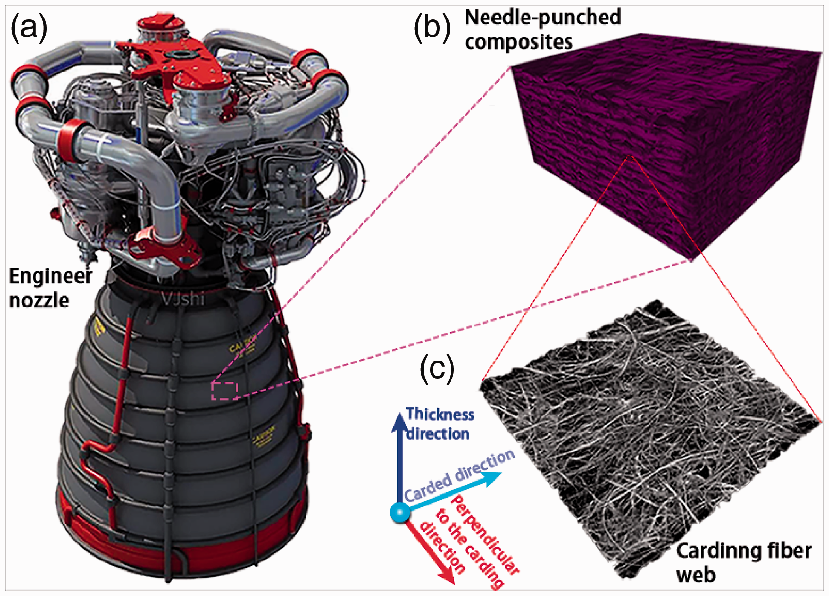
Application of the carding fiber web: (a) engine nozzle; (b) needle-punched composites; (c) the carding fiber web.

Due to the presence of the randomly distributed fibers and large slenderness ratio fibers (LSRFs) in the carding fiber web, it is difficult to construct the high-fidelity three-dimensional (3D) model of the CQFW. Recent studies on the methods of constructing a 3D carding fiber web model (CFWM) mainly included the random sequential adsorption method (RSAM)^10–15 and the modified RSAM,¹⁶ deposition method,^17–19 Monte Carlo method,^20,21 the force-biased method^22,23 and reconstructed 3D model method based on the microcomputed tomography image.^24–27 However, the methods above^10–27 mainly aimed at establishing the short and straight fibers or the small slenderness ratio fibers to construct the fiber web model, the actual carding fiber web contains not only straight fibers but also curved LSRFs.^2,10 In comparison to the fiber aggregation with short-straight fibers and small slenderness ratio fibers, the carding fiber web with curved LSRFs (slenderness ratio more than 1000) imply the complex space geometry structure. Randomly distributed fibers in the carding fiber web causes the irregular spatial pores.²⁸ To solve the problem of mutual penetrations among adjacent fibers²⁹ in the carding fiber web, complex geometry algorithms and solid programming computer acknowledgements are required, especially considering the LSRFs in the carding fiber web. Furthermore, even if such a modeling program based on complex geometry algorithms is conducted, the majority of the modeling time is consumed to detect the overlap between fibers in yarns.³⁰ Therefore, a method which can predict and design the ATC and illustrate the detailed heat conduction behavior of the carding fiber web is urgently needed.

In addition, the finite element analysis on the performance of the fiber web focused on the mechanical properties of its composites,^12,31–33 or aimed to simulate the needle-punched process.³⁴ Few studies^10,35 aimed to establish the 3D model of the carding fiber web containing LSRFs and analyze its detailed AHT (including temperature distribution (TD) and heat flux distribution (HFD)).

Based on the urgent need, a ‘three-step’ method is proposed to generate a 3D CFWM containing LSRFs in this study. The 3D finite element model of the CQFW for heat transferring analysis is established. Meanwhile, the matching air matrix model in it, which is the solid element model, is obtained through Boolean operation in finite element software (FES). A 3D CFWM is assembled with a solid air model to form the two-phase composite model of heat transmission, and the AHT of the carding fiber web is further analyzed in detail. Compared with the methods mentioned above,^10–27 the method proposed in this paper can not only obtain the detailed temperature and HFD, but also carry out the mechanical analysis of the CQFW and its composites efficiently and precisely. Moreover, compared with the models containing short and straight fibers mentioned above, the CQFW containing LSRFs in this paper can more clearly illustrate the relationship between the fiber orientation and HFD. In addition, the ‘three-step’ method is more efficient and low cost due to the broad application of the Python language in FES. Therefore, this method can promote the development of the research and engineer application of the CQFW significantly.

Experimental details

Materials

The CQFWs (shown in Figure 1(c)) used in this study were supplied by Tianjin Gongda Aerotech Composite Materials Co., Ltd. The detailed information on the CQFW and the quartz fiber are listed in Table 1. In addition, thermal conductivity of the air is 0.026 W/m · K in the finite element analysis. As shown in Figure 1, the CQFWs were used to make the needle-punched composites shown in Figure 1(b). Furthermore, the needle-punched composites were used to make the engineer nozzle as shown in Figure 1(a).

Table 1.

The detailed information on the CQFW and quartz fibers

Carding quartz fiber webs	Areal density (g/m²)	Thickness (mm)
Carding quartz fiber webs	18.3	0.35
	Diameter (μm)	Thermal conductivity (W/m · K)	Density (g/cm³)
Quartz fibers	7	1.38	2.2

CQFW: carding quartz fiber web.

Measurements of thickness and areal density

Figure 2 shows the detailed measurements of areal density and thickness of the CQFW. The carding fiber web was cut by the disk sampler shown in Figure 2(a) to obtain six circle samples at 100 cm² (shown in Figure 2(b)). The digital thickness tester shown in Figure 2(c) was used to measure the thickness of the circle samples. The electronic scale shown in Figure 2(d) was used to measure the mass of the circle samples and then the areal density of the CQFW was obtained. Six specimens, as shown in Figure 2(b), were tested to obtain the thickness and areal density; furthermore, the corresponding mean values were calculated as the final results and recorded in Table 1. Measurements of thickness are according to the standard GB/T3819-1997.

Figure 2.

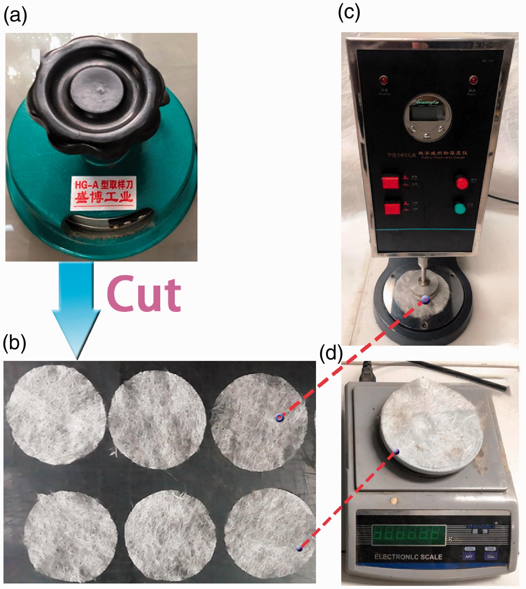
Measurements of areal density and thickness of the carding quartz fiber web (CQFW): (a) disk sampler; (b) samples for testing; (c) measuring the thickness of the CQFW; (d) measuring the areal density of the CQFW.

Statistical analysis

Figure 3 illustrates the statistical analysis process. A 3D profilometer was used to observe the geometric morphology of fibers in the CQFW. As can be seen in Figure 3a(I), most of the fibers in the carding fiber web tend to be concentrated in one direction, that is, the carding direction as shown in Figure 3a(I), which is also the forward direction of the carding fiber web in the carding machine. Furthermore, the geometric morphologies of fibers in the CQFW are curved fibers mixed with straight fibers as shown in Figure 3a(II). The fiber length distribution is shown in Figure 3(b), and it can be seen that the ratio of fibers at 71–80 mm is more than 25%. Moreover, the concrete distribution of the fiber orientation is illustrated in Figure 3(c), measured by the DHU-11 fiber orientation analyzer.^7,10,35 The orientation angle range of most of the fibers is from 60° to 90° as can be seen in Figure 3(c). The measurement of the distribution of the fiber orientation is according to the standard GB/T 30967-2014.

Figure 3.

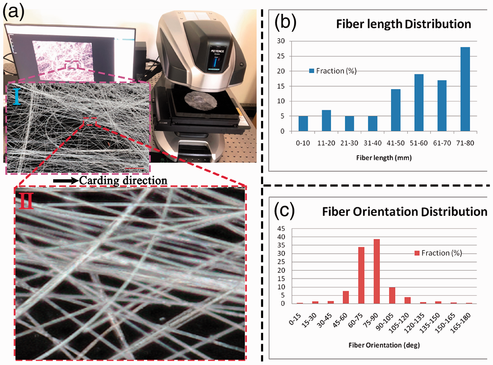
Statistical analysis of the carding quartz fiber felt: (a) morphology observation using three-dimensional (3D) profilometer, (I) enlarged view 1, (II) enlarged view 2; (b) fiber length distribution of the carding fiber web; (c) fiber orient distribution of the carding fiber web.

Measurements of the ATC

A hot-disk thermal analyzer (model TPS 3500) shown in Figure 4(a) was used to measure the ATC of the CQFW. As the measurement of the ATC requires the specific heat of the CQFW as the input parameter, thus, the specific heat of the CQFW needs measuring before measuring the ATC of that as shown in Figure 4(b1). The CQFWs were sheared into the circular as the samples for measuring specific heat as shown in Figure 4(b2). The goldware sensor for measuring specific heat is shown in Figure 4(b3) and its diameter Ds is 20 mm, which is also the diameter of samples shown in Figure 4(b2). The samples were stacked to be 15 mm and then loaded into the goldware sensor for the specific heat test. The measurement of the ATC of the CQFW can be seen in Figure 4(c1), its testing samples at 65 × 65 × 25 mm³ are displayed in Figure 4(c2), and the anisotropic sensor 101472 is shown in Figure 4(c3). The sensor was caught in the middle of two same samples as shown in Figure 4(c1). Furthermore, the ATC; that is, the thermal conductivity of the carding direction in plane, the thermal conductivity of the direction perpendicular to the carding direction in plane, and the thermal conductivity of the thickness direction were measured. Measurements of ATC were carried out five times based on five groups of samples, and then the average values were calculated and recorded in Table 3. The thermal conductivity test is according to the standard ISO 22007-2:2008(E). The relationship between unidirectional thermal conductivity (λ), specific heat (c), apparent density (ρ′) and thermal diffusion coefficient (A) can be demonstrated by equation (1):

λ = ρ ′ Ac

(1)

Figure 4.

Measurements of the specific heat and anisotropic thermal conductivity of the carding quartz fiber web (CQFW): (a) hot-disk thermal analyzer; (b1) measurement of the specific heat of the CQFW; (b2) samples for measuring the specific heat of the CQFW; (b3) sensor for measuring the specific heat of the CQFW; (c1) measurement of the anisotropic thermal conductivity (ATC) of the CQFW; (c2) samples for measuring the ATC of the CQFW; (c3) sensor for measuring the ATC of the CQFW.

Finite element analysis on heat transfer of CQFW

Spatial layer fiber growth model

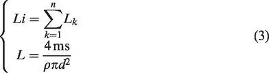
Based on the results of the statistical analysis of CQFW in the Materials and Statistical analysis sections, the Python script for generating the spatial layer fiber model (SLFM) is created and run in FES to generate the SLFM. The workflow of the script, which includes four steps, is illustrated in Figure 5. First, as can be seen in Figure 5, the geometry morphology (curved or straight line) of the fiber model is chosen randomly from the morphology distribution list constructed by the statistical analysis, the curved fiber is controlled by equation (2), which is called a catenary equation in the engineering application. In equation (2), parameters x and y are the x coordinate value and y coordinate value of the catenary curve Cartesian coordinate system, parameter a is the catenary coefficient, fibers at different bending degrees (curved type I, II, III, as shown in Figure 5) can be obtained by altering the catenary coefficient a; second, the fiber length is chosen randomly from the length distribution list constructed by the statistical analysis as shown in Figure 3(b), then one fiber no. n (n is a positive integer) with determined geometry and length is established; third, fiber no. n is translated to the spatial plane which is n × d from the original plane, d is the diameter of the fiber model. An angle α° is chosen randomly from the fiber orientation list constructed by the statistical analysis as shown in Figurre 3(c), and fiber no. n is rotated an angle α°; fourth, judge whether the total length of the generated fibers Li reaches the set length value L, if Li ≥ L, the script ends running and the SLFM is obtained, if not, then back to the first step to continue generating the fiber no. n + 1, until the set condition Li ≥ L is met, then the script is over and SLFM is established as shown in Figure 6. Li and L are calculated by equation (3). In equation (3), L _k is the length of random fiber no. n, s is the area of the XY plane of the SLFM, m is the areal density of the experimental carding fiber web and ρ is the density of the quartz fiber.

y = a (\frac{{e^{\frac{x}{a}} + e}^{- \frac{x}{a}}}{2} - 1)

(2)

\{\begin{array}{l} L i = \sum_{k = 1}^{n} L_{k} \\ L = \frac{4 ms}{ρ π d^{2}} \end{array}

(3)

Figure 5.

Python script flow of spatial layering fiber growth model.

Figure 6.

Display of the spatial layer fiber model (SLFM) from a different view: (a) XY plane view; (b) ZX plane view; (c) ZY plane view.

Figure 6(a), (b) and (c) is, respectively, the view of the XY plane, ZX plane and ZY plane of the SFWM. The spatial laying characteristic can be observed clearly from Figure 6(b) and (c). For highlighting the spatial laying characteristic, the fiber quantity displayed in Figure 6 is 1116 fibers which are much more than the fiber quantity of practical CFWM shown in Figure 7(a).

Figure 7.

Fiber compression and deposition process by the explicit method. (a) Deposition and compression of the spatial layer fiber model (SLFM); (b1)–(b4) different states of deposition and compression process of the SLFM; (c) carding fiber web model after deposition and compression.

Deposition and compression process by the explicit method

Gravity is applied to the SLFM that is shown in Figure 6, furthermore, the compression plate as shown in Figure 7(a) is established to compress the fibers, the deposition plate is fixed, then the deposition and compression process is conducted by the explicit method of FES. The concrete material properties and applied conditions during the deposition and compression process are clarified in our previous work.¹⁰ Different deposition and compression states can be observed in Figure 7(b1) to (b4). It can be observed in Figure 7(b1) and (b2) that the fibers lap and contact with each other, and no fiber mosaic occurred in the deposition and compression process, then the high-fidelity model of the carding fiber web is established as shown in Figure 7(c), and the detailed display of fibers contacting with no mosaic can also be seen in Figure 7(c). Before proceeding with the deposition and compression process, one node set containing all the nodes of one fiber should be created one by one. Furthermore, the corresponding nodes are defined to output their current 3D displacement data and coordinate data, providing the sweep path data for the CFWM of solid elements.

Finite element model of heat transfer of carding fiber web

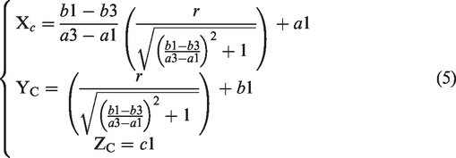
Considering that the AHT model should be the solid element model, the CFWM of the beam element shown in Figure 7(c) needs converting to that of the solid element. During the converting process, Python script is adopted to extract the displacement values of the corresponding nodes of the fiber model from the ODB file as shown in Figure 8(a). 3D coordinate data of the nodes of one fiber can be calculated based on the displacement values as the solid sweep path points. In addition, the sweep datum plane M and the starting point O are required before the sweep, the starting point O is illustrated in Figure 8a(II), points A, C and O all belong to datum plane M. As is demonstrated in Figure 8a(II), coordinate values of the points O and B are (a1, b1, c1) and (a3, b3, c3), respectively, that is, are the coordinate values of node 1 and node 2 in the node-set shown in Figure 8a(I). The distance between points O and A is the fiber radius r, thus the coordinate value of point A is (a1, b1, c1 + r). Points A, B and O all belong to the plane M′, which is perpendicular to the datum plane M. Therefore, based on the principle of determining plane by three points, the datum plane M can be determined by solving the coordinate value of point C (X _c , Y _c , Z _c ). The mathematical relationship between the vector 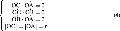$\vec{OA}$ , $\vec{OB}$ and $\vec{OC}$ can be expressed by equation (4). Taking the known coordinate values into equation (4), and then the coordinate values of point C are solved as listed in equation (5). Finally, points O, A and B determine the datum plane M, the solid-sweep function is adopted to sweep along the solid sweep path points based on the datum plane M, the fiber model of beam elements is then converted into that of solid elements, that is illustrated by:

\{\begin{matrix} \vec{OC} \cdot \vec{OA} = 0 \\ \vec{OC} \cdot \vec{OB} = 0 \\ \vec{OB} \cdot \vec{OA} = 0 \\ | \vec{OC} | = | \vec{OA} | = r \end{matrix}

(4)

Figure 8.

Establishment of finite element model of the three-dimensional (3D) carding quartz fiber web (CQFW) for heat transmission: (a) reconstruction of the 3D CFWM; (b) geometry model of the 3D CQFW; (c) finite element model of the 3D CQFW.

Figure 8a(I) to 8a(II), then the CFWM of the solid element shown in Figure 8(b) is obtained by geometric Boolean operation in FES. The solid fiber model is combined with the solid air model to form the two-phase AHT model as shown in Figure 8(b). Fibers and air models are meshed by free meshing technology, then the finite element heat transferring model of the carding fiber web shown in Figure 8(c) is reconstructed. Detailed information on the finite element model of the CQFW is shown in Table 2.

\{\begin{array}{l} X_{c} = \frac{b 1 - b 3}{a 3 - a 1} (\frac{r}{\sqrt{{(\frac{b 1 - b 3}{a 3 - a 1})}^{2} + 1}}) + a 1 \\ Y_{C} = (\frac{r}{\sqrt{{(\frac{b 1 - b 3}{a 3 - a 1})}^{2} + 1}}) + b 1 \\ Z_{C} = c 1 \end{array}

(5)

Table 2.

Detailed information of the finite element heat transferring model of the CQFW

FEM model	Element number (×10⁶)	Element type	Meshing method	Model size (mm³)	Diameter of fiber model (mm)	Fiber volume content (%)
Quartz carding fiber web	8.091351	DC3D4	Free meshing	10 × 10 × 0.7	0.028	2.38

CQFW: carding quartz fiber web; FEM: finite element method.

Temperature periodic boundary conditions

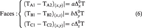
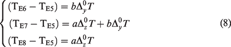
Steady heat conduction is carried out to analyze the AHT of the CQFW in FES, and temperature periodic boundary conditions (TPBCs) are applied to the finite element model of the carding fiber model. Figure 9 is the schematic diagram of the nodal position and geometric feature labels by applying the TPBCs. The application of TPBCs can be divided into three types: nodes on opposite parallel surfaces (face A1 and A2 in Figure 9), nodes on parallel edges (edges E1, E2, E3 and E4 in Figure 9) and nodes on the corresponding vertex (nos 1–8 in Figure 9). The constraint equations for applying TPBCs are summarized as follows in equation (6) to equation (10). In equations (6) to (10), a, b and c are the lengths along the z, y, x directions of the cube cell, respectively, as shown in Figure 9.

Faces: \{\begin{array}{l} (T_{A 1} - T_{A 2}) ‖_{(x, y)}| = a Δ_{x}^{0} T \\ (T_{B 1} - T_{B 2}) ‖_{(x, z)}| = b Δ_{y}^{0} T \\ (T_{C 1} - T_{C 2}) ‖_{(x, y)}| = c Δ_{z}^{0} T \end{array}

(6)

Edges: \{\begin{array}{l} (T_{E 2} - T_{E 1}) = a Δ_{z}^{0} T \\ (T_{E 3} - T_{E 1}) = a Δ_{z}^{0} T + c Δ_{x}^{0} T \\ (T_{E 4} - T_{E 1}) = c Δ_{x}^{0} T \end{array}

(7)

\{\begin{array}{l} (T_{E 6} - T_{E 5}) = b Δ_{y}^{0} T \\ (T_{E 7} - T_{E 5}) = a Δ_{z}^{0} T + b Δ_{y}^{0} T \\ (T_{E 8} - T_{E 5}) = a Δ_{z}^{0} T \end{array}

(8)

\{\begin{array}{l} (T_{E 10} - T_{E 9}) = b Δ_{y}^{0} T \\ (T_{E 11} - T_{E 9}) = a Δ_{z}^{0} T + c Δ_{x}^{0} T \\ (T_{E 12} - T_{E 9}) = c Δ_{x}^{0} T \end{array}

(9)

Figure 9.

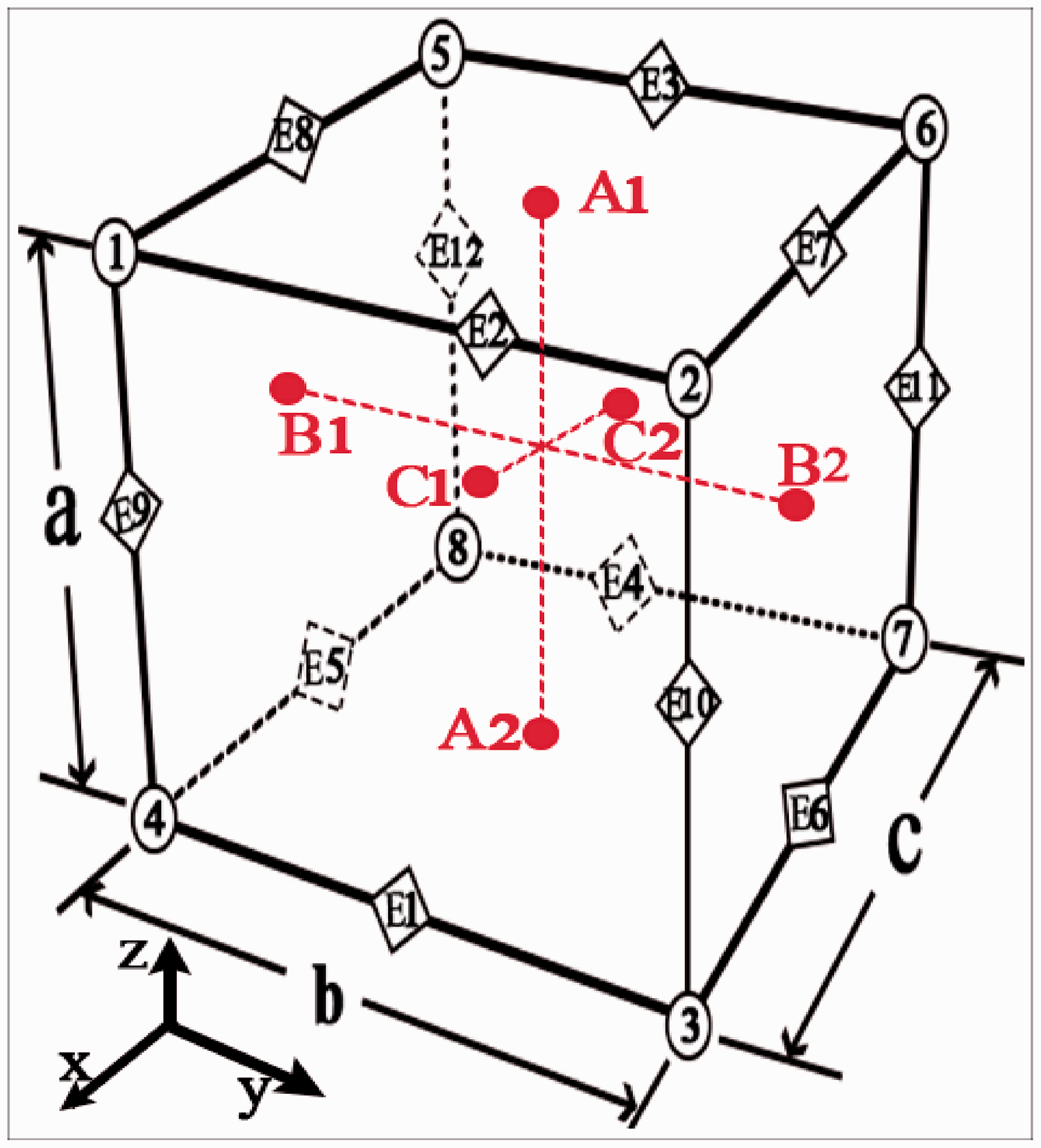
Nodal position and geometric feature numbering of cubic periodic boundary conditions.

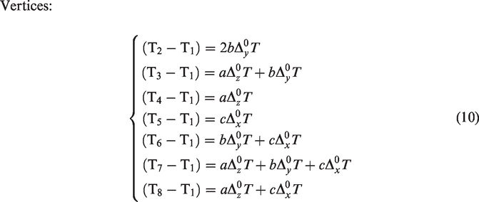
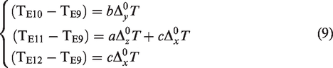
(x, y) in equation (6) refers to the xy plane as shown in Figure 9. Similarly, (x, z) and (y, z), respectively, represent the xz plane and yz plane as shown in Figure 9. $Δ_{x}^{0} T$ , $Δ_{y}^{0} T$ and $Δ_{z}^{0} T$ are the temperature gradients (TGs), which are, respectively, parallel to the x, y, and z axial in Figure 9. T_A1, T_B1 and T_C1, respectively, represent the temperature of the nodes (master nodes) on boundary faces A1, B1 and C1 as shown in Figure 9. Similarly, T_A2, T_B2 and T_C2, respectively, represent the temperatures of the nodes (slave nodes) on boundary faces A2, B2 and C2 as shown in Figure 9. T_E _i (i ∈ [1,12]) represents the temperature of the nodes on the edges E1 to E12 as shown in Figure 9. T _n (n ∈ [1,8]) represents the temperature of the eight vertex nodes as shown in Figure 9.

\{\begin{array}{l} (T_{2} - T_{1}) = 2 b Δ_{y}^{0} T \\ (T_{3} - T_{1}) = a Δ_{z}^{0} T + b Δ_{y}^{0} T \\ (T_{4} - T_{1}) = a Δ_{z}^{0} T \\ (T_{5} - T_{1}) = c Δ_{x}^{0} T \\ (T_{6} - T_{1}) = b Δ_{y}^{0} T + c Δ_{x}^{0} T \\ (T_{7} - T_{1}) = a Δ_{z}^{0} T + b Δ_{y}^{0} T + c Δ_{x}^{0} T \\ (T_{8} - T_{1}) = a Δ_{z}^{0} T + c Δ_{x}^{0} T \end{array}

(10)

Equation (6) is the constraint equation on opposite parallel surfaces A1 and A2, parallel surfaces B1 and B2, parallel surfaces C1 and C2, as shown in Figure 9. Equation (7) is the constraint equation of edges 1, 2, 3 and 4 shown in Figure 9. Similarly, equation (8) is the constraint equation of edges 5, 6, 7 and 8. Equation (9) is the constraint equation of edges 9, 10, 11 and 12. Equation (10) is the constraint equation of nodes 1, 2, 3, 4, 5, 6, 7 and 8 on the corresponding vertex as shown in Figure 9.

In addition, the thermal conductivity was calculated according to the Fourier law. The Python language was used to extract the nodal temperature to perform the calculation.

Results and discussion

Convergence study of mesh density

As is known to all, meshing density can greatly affect the numerical results. Therefore, aiming at studying the relationship between meshing density and computational convergence is essential. Figure 10(a) is the curve of the thermal conductivity of the finite element model of the CQFW along the carding direction versus different element numbers of the finite element model of the CQFW. Figure 10(b1) to (b4) shows the TD of the finite element model of the CQFW along the same direction with different element numbers (mesh sizes). Figure 10(a) reveals that there has been a gradual increase in the thermal conductivity with an increment of element numbers, and the overall trend in Figure 10(a) presents the obvious convergence characteristic. Actually, the thermal conductivity at 5.180922 × 10⁶ elements (mesh size 0.07 in Figure 10(a)) is 0.06544 W/m·K, it is almost equal to 0.06551 W/m·K, which is the thermal conductivity at 8.091351 × 10⁶ elements (mesh size 0.05 in Figure 10(a)). Consequently, the mesh size of this finite element simulation is finally determined to be 0.05.

Figure 10.

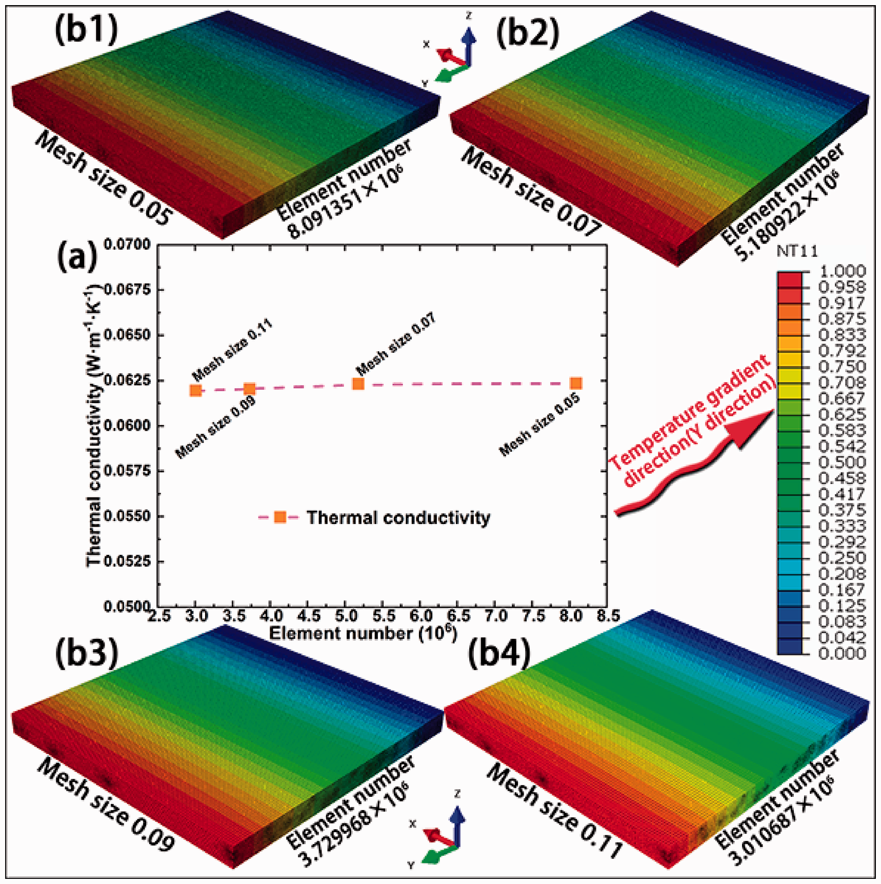
Analysis on computational convergence and different mesh size (element number). (a) Thermal conductivity of carding direction (finite element method) versus different element numbers (mesh size) of the carding fiber web model (CFWM); (b1)–(b4) temperature distribution (TD) of the CFWM at different mesh sizes (element numbers).

Analysis on ATC of the CQFW

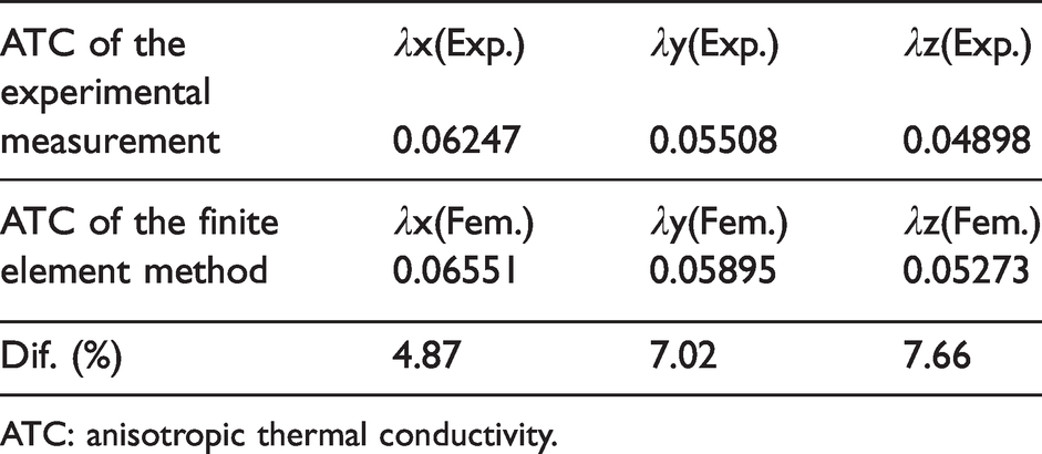
Experimental and numerical results of the ATC of the CQFW are recorded in Table 3. λx(Exp.), λy(Exp.) and λz(Exp.) are, respectively, the experimental thermal conductivity of the carding direction in plane, the direction perpendicular to the carding direction in plane and the thickness direction. Similarly, λx(Fem.), λy(Fem.) and λz(Fem.) are, respectively, the numerical thermal conductivity along such three directions. It can be observed from Table 3 that both the experimental and the numerical results all present obvious anisotropy of the thermal conductivity. Such anisotropy can be observed in Figure 11 more obviously, which is the curve of ATC of the experimental and finite element method. Moreover, it is clear in Figure 11 that the thermal conductivity of the carding direction in plane λx is the maximum among the three, and that of the thickness direction λz is the minimum. In addition, it can be found straight from Figure 11 and Table 3 that the thermal conductivity of the finite element method is slightly larger than that of the experimental measurement in three directions; we speculate that it might be because the heat transmission between air and fibers is ideal with no thermal resistance. Significantly, as can be seen in Table 3, the absolute error values in three directions between the experimental and numerical results are, respectively, 4.87%, 7.02% and 7.66%, which are all less than 8%, that is, there is a good agreement between the experimental and numerical results, thus it can be concluded that the finite element model of anisotropic heat conduction of the CQFW is accurate and reliable.

Table 3.

ATC of the experimental and numerical method

ATC of the experimental measurement	λx(Exp.)	λy(Exp.)	λz(Exp.)
ATC of the experimental measurement	0.06247	0.05508	0.04898
ATC of the finite element method	λx(Fem.)	λy(Fem.)	λz(Fem.)
ATC of the finite element method	0.06551	0.05895	0.05273
Dif. (%)	4.87	7.02	7.66

ATC: anisotropic thermal conductivity.

Figure 11.

Curve of anisotropic thermal conductivity (ATC) of the experimental and finite element method.

Figure 12(a) and (b), respectively, show the TD of applying the TG along the carding and thickness direction. As shown in Figure 12(a)(I) and (a)(II), not only in the assembly but also in the fibers individually, the TD along the carding direction (direction of applying TG) shows the gradual decrement characteristic; however, it presents an isothermal property at the direction perpendicular to the carding direction in the XY plane, or at the thickness direction. Such a TD characteristic is further to be illustrated in detail in Figure 12(a)(III) and (a)(IV). Figure 12(a)(III) is the multi-cut view of the TD, Figure 12(a)(IV) is the curve of the nodal temperature versus displacement, which is corresponding with the nodes a1, a2, a3 in Figure 12(a)(III). Temperature from point a3 to point a1 decreases gradually. Temperature at point a1 and a2 is equal, which is 0.5°C as shown in Figure 12(a)(IV).When the TG is applied to the thickness direction, the same TD characteristic can be observed as shown in Figure 12(b)(I), (II), (III) and (IV). Similarly, the same TD characteristic can be observed when TG is applied to the Y direction.

Figure 12.

Temperature distribution (TD) of the carding fiber felt along different directions. (a) Along carding (X) direction: (I) assembly; (II) fibers; (III) multi-cut view; (IV) detailed TD characterization curve; (b) Along thickness (Z) direction: (I) assembly; (II) fibers; (III) multi-cut view; (IV) detailed TD characterization curve.

Figure 13(a1), (b1), (c1) are the HFD of applying TG to the carding (X) direction, the Y direction and the thickness direction, respectively. The air matrix is removed to display the HFD in fibers individually as shown in Figure 13(a2), (b2), (c2). As shown in Figure 13(a2), the HFD presents the characteristic that, the more consistent with the direction applying the TG the fiber axial direction is, the higher is the heat flux value in the fiber. In other words, the smaller the angle between the fiber axial direction and the direction applying the TG, the higher is the heat flux value in the fiber. Such HFD characteristic is more obvious in Figure 13(b2). In order to clarify such HFD characteristic in detail, Figure 13(a2) is enlarged to be displayed in Figure 14(a); furthermore, heat flux values of fibers with different axial orientation are quantified by curves as demonstrated in Figure 14(b). As illustrated in Figure 14(a), the angle between the axial direction of fiber A and the direction applying the TG is smaller than those between the axial direction of fibers B or C and the direction applying the TG. Consequently, the heat flux values in fiber A are higher than those in fibers B and C, the corresponding heat flux value curve is shown in Figure 14(b). As shown in Figure 14(b), the heat flux value of node A1 in fiber A is higher than those of node B1 in fiber B and node C1 in fiber C, node A1, B1 and C1 are equal in the Y coordinate value. Similarly, the same value relationship of heat flux can also be observed in nodes A2, C2, and B2, or in nodes A3, C3, and B3. Significantly, the angle between the axial direction of fiber B and the direction applying the TG is larger than those between the axial directions of fibers A or C and the direction applying the TG, therefore, the heat flux value in fiber B is the smallest among the three as shown in Figure 14(b). The reason for such HFD characteristics is that the smaller angle between the fiber axial direction and the direction applying TG means the more consistent orientation, that is, the smaller angle means the smaller thermal resistance, thus that leads to the higher heat flux value. In addition, the heat transmission along the thickness direction is among fiber radial directions, fiber axial orientation has no obvious effects on the HFD along the thickness direction, thus the HFD along the thickness direction presents more evenly distributed than those along the X or Y direction as shown in Figure 13.

Figure 13.

Heat flux distribution (HFD) of the carding fiber felt along different directions: (a1) assembly along the carding (X) direction; (a2) fibers along the carding (X) direction; (b1) assembly perpendicular to the carding direction; (b2) fibers perpendicular to the carding direction; (c1) assembly along the thickness (Z) direction; (c2) fibers along the thickness (Z) direction.

Figure 14.

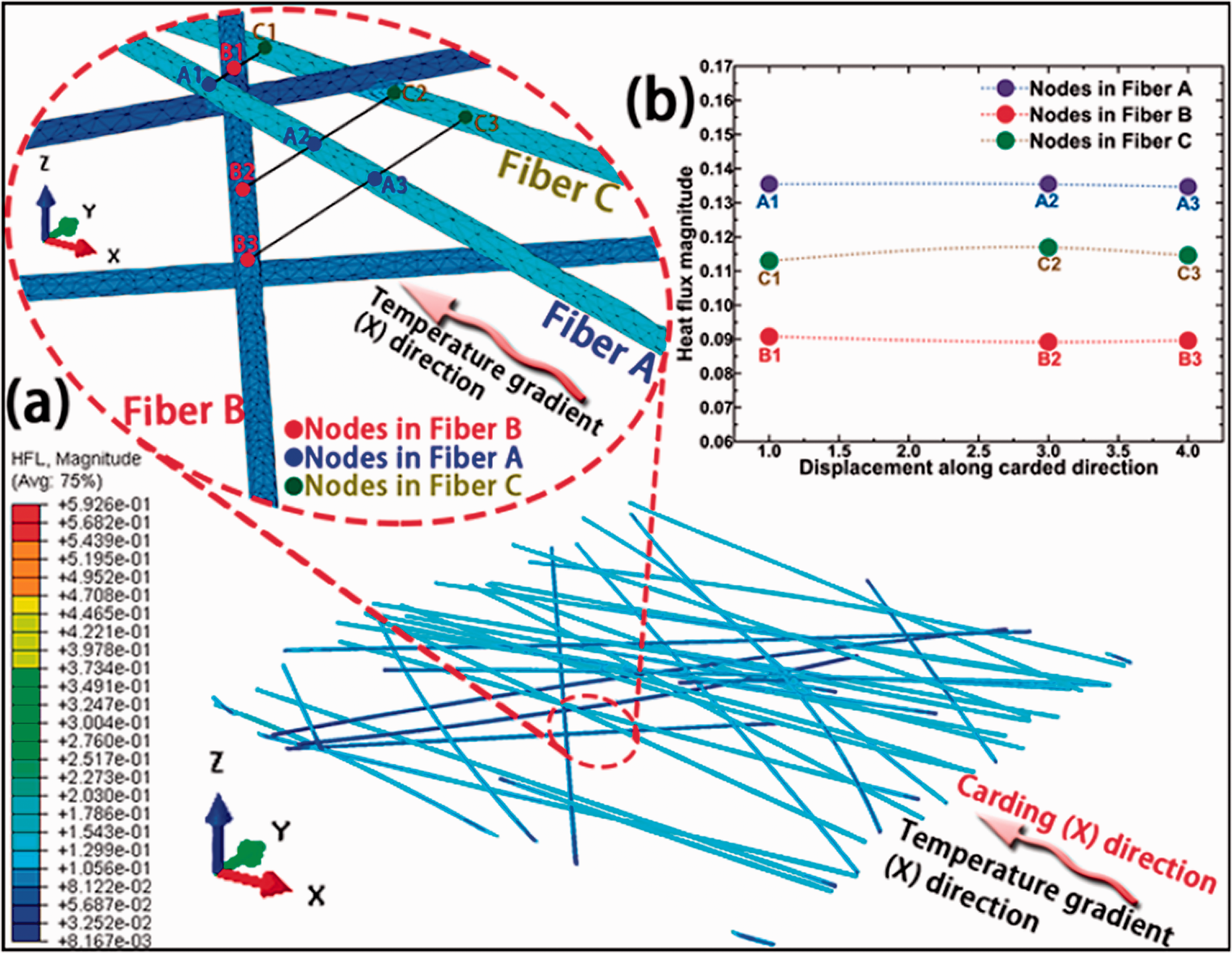
Detailed heat flux distribution (HFD) along the carding (X or TG) direction in fibers. (a) Enlarged view of HFD of fibers A, B and C; (b) curve of heat flux magnitude at different displacements (nodes) in different fibers.

Conclusions

Based on the broad application of the Python language in pre and post-processing of FES, a ‘three-step’ method is proposed to establish the finite element model of heat transmission of the carding fiber web containing LSRFs. Furthermore, the analysis of anisotropic thermal conduction of the CQFW is carried out by the explicit method of the FES based on the established model. Detailed TD and HFD are analyzed through steady heat conduction and ATC is predicted. Moreover, the anisotropic module of the hot-disk thermal analyzer is used to measure the ATC of the CQFW. The numerical results are entirely consistent with the experimental results, indicating that the model established is accurate and reliable. Although the study results are specific to the CQFW, the study method can be used generally to other fibrous materials with randomly distributed fibers and LSRFs. In addition, the finite element model of the needle-punched preform that contains the CQFW can be established in our further work. Furthermore, the thermal conduction of the needle-punched preforms can be analyzed in detail. The principal conclusions of this paper are summarized as follows:

Both the numerical results and the experimental results show obvious anisotropic characteristics of the thermal conductivity. To be specific, thermal conductivity of the carding direction in web plane > thermal conductivity of the direction perpendicular to the carding direction in web plane >thermal conductivity of the thickness direction.

The maximum of the absolute error between the numerical and experimental thermal conductivity is 7.66% in the thickness direction. Furthermore, the minimum is 4.87% in the carding direction between between the numerical and experimental thermal conductivity. The absolute error values of 3D ATC among the experimental and numerical results are all less than 8%, thus it can be concluded that the finite element model of heat transferring of the carding fiber web in this study is accurate and reliable.

The TD along the direction applying the TG decreases uniformly and graduall; however, it presents an apparent isothermal property along the direction perpendicular to the direction applying the TG.

Distribution of the fiber orientation in the web plane has significant effects on the HFD. In particular, the smaller the angle between the fiber axial direction and the direction applying the TG is, the higher is the heat flux value in the fiber.

The HFD along the thickness direction is more uniform than that in the fiber web plane, that is because the heat transmission in the thickness direction is mainly between the fiber radial directions. However, heat transmission in the fiber web plane exists in both the fiber axial and radial directions. In a word, the heat transmission form along the thickness direction is more singular compared with that in the plane of the carding fiber web, and such singling of the heat transmission form finally results in the more uniform distribution of the heat flux along the thickness direction.

Footnotes

Declaration of conflicting interests

The author(s) declared no potential conflicts of interest with respect to the research, authorship, and/or publication of this article.

Funding

The author(s) disclosed receipt of the following financial support for the research, authorship, and/or publication of this article: This work was finally supported by the Scientific Research Project of Tianjin Education Commission (2017KJ066); the Major Science and Technology Projects of Tianjin (18ZXJMTG00190); the Major Science and Technology Projects of Shanxi Province (20181102022) and the University Innovation Team Training Plan of Tianjin (TD13-5043).

ORCID iDs

Peijian Du

Xiang Ding

References

Yang

Chen

, et al. Comparing the uniformity of light glass fiber felt based on process improvement, microstructural forming mechanism and physical properties. Text Res J 2018; 89: 3447–3456.

Zeng

Shen

Duan

, et al. Properties of MWCNT – glass fiber fabric multiscale composites: mechanical properties, interlaminar adhesion, and thermal conductivity. Text Res J 2017; 88: 2712–2726.

Hsing

W-H

Lin

J-H

Kao

K-T.

The investigation of fiber carding performance with the application of static electricity to carded nonwoven fabric process. J Mater Process Technol 2007; 192: 543–548.

Miao

Glassey

HE.

An experimental study of the needled nonwoven process part I: fiber geometry before needle punching. Text Res J 2004; 74: 329–332.

Chen

Zhang

, et al. Three-dimensional needle-punching forcomposites – a review. Compos Pt A-Appl Sci Manuf 2016; 85: 12–30.

Chen

Xie

, et al. Damage evaluation of quartz woven fabrics during needle punching process. J Ind Text 2020; 1–27.

Wang

, et al. Damage characterization of quartz woven fabric and the change of the fiber distribution orientation of the needle punched quartz fiber felt. Acta Materiae Compositae Sinica 2020; 13: 34–44.

Zhou

X-Y

Ruan

Zhang

, et al. Design optimization for thermal conductivity of plain-woven textile composites. Compos Struct 2021; 255: 112830.

Dai

Y-J

Tang

Y-Q

Fang

W-Z

, et al. A theoretical model for the effectivethermal conductivity of silica aerogel composites. Appl Therm Eng 2017; 128: 1634–1645.

10.

Chen

X-M

C-Y

Xie

, et al. 3D modeling of carded fiber web based on Abaqus/Python. J Tiangong University 2021; 40: 34–39.

11.

Chapelle

Lévesque

Brøndsted

, et al. Generation of non-overlapping fiber architecture. 20th International Conference on Composite Materials. Copenhagen: ICCM, 2015, pp. 1–12.

12.

Song

Zhang

Chen

, et al. Three-dimensional finite element models and tensile properties of carbon fiber needled felt reinforced composites. J Ind Text 2019; 50: 293–311.

13.

Tian

Zhou

JM.

Numerical evaluation of effective elastic properties of composites reinforced by spatially randomly distributed short fibers with certain aspect ratio. Compos Struct 2015; 131: 843–851.

14.

Tian

Zhou

, et al. Representative volume element for composites reinforced by spatially randomly distributed discontinuous fibers and its applications. Compos Struct 2015; 131: 366–373.

15.

Islam

Tudryn

Picu

. Microstructure modeling of random composites with cylindrical inclusions having high volume fraction and broad aspect ratio distribution. Comput Mater Sci 2016; 125: 309–318.

16.

Lucian

Pelegri

AA.

Numerical generation of a random chopped fiber composite RVE and its elastic properties. Compos Sci Technol 2008, 68: 2792–2798.

17.

Provatas

Haataja

Asikainen

, et al. Fiber deposition models in two and three spatial dimensions. Colloids Surf A Physicochem Eng Asp 2000; 165: 209–229.

18.

Kari

Berger

Gabbert

Numerical evaluation of effective material properties of randomly distributed short cylindrical fiber composites. Comput Mater Sci 2007, 39: 198–204.

19.

Ekman

Miettinen

Turpeinen

, et al. The number of contacts in random fibre networks. Nord Pulp Paper Res J 2012; 27: 270–276.

20.

Duschlbauer

Bohm

Heinz

Computational simulation of composites reinforced by planar random fibers: homogenization and localization by unit cell and mean field approaches. J Compos Mater 2006; 40: 2217–2234.

21.

Gusev

Heggli

Lusti

, et al. Orientation averaging for stiffness and thermal expansion of short fiber composites. Adv Eng Mater 2002, 4: 931–933.

22.

Altendrof

Jeulin

Random-walk-based stochastic modeling of three-dimensional fiber systems. Phys Rev E 2011; 83: 041804.

23.

Harper

Qian

Luchoo

, et al. 3D geometric modelling of discontinuous fibre composites using a force-directed algorithm. J Compos Mater 2017; 51: 2389–2406.

24.

Vecchio

Image based characterization and geometric modelling of 3D materials microstructures. PhD Thesis. Kaiserslautern, Gemany: Technische Universitot Kaiserslautern, 2015.

25.

Soltani

Johari

Zarrebini

Effect of 3D fiber orientation on permeability of realistic fibrous porous networks. Powder Technol 2014; 254: 44–56.

26.

Yildiz

Evaluation of nano-filler dispersion quality in polymeric films with binary feature characteristics and fractal analysis.

IET Image Processing 2020; 14: 2006–2012.

27.

Yildiz

Application of image processing for quantization and characterization of fabrics with polymeric coatings.

Pamukkale University J 2018; 24: 255–259.

28.

Huang

Didari

Wang

, et al. Generalized periodic surface model and its application in designing fibrous porous media. Engng Comput 2015; 32: 7–36.

29.

Gaiselmann

Froning

Totzke

, et al. Stochastic 3D modeling of non-woven materials with wet-proofing agent. Int J Hydrogen Energy 2013; 38: 8448–8460.

30.

Huang

Wang

Miao

, et al. Dynamic relaxation approach with periodic boundary conditions in determining the 3-D woven textile micro-geometry. Compos Struct 2013; 106: 417–425.

31.

Xie

Liang

Fang

, et al. Effect of needling parameters on the effectiveproperties of 3D needled C/C-SiC composites. Compos Sci Technol 2015; 117: 69–77.

32.

Fan

Meng

, et al. Modal analysis of 3D needled waste cotton fiber/epoxy composites with experimental and numerical methods. Text Res J 2020; 91: 358–372.

33.

Meng

Fan

Wan

, et al. Production of three-dimensional fiberneedle-punching composites from denim waste for utilization as furniture materials. J Clean Prod 2021; 281: 125321.

34.

Xie

Chen, Zhang

, et al. Experimental and numerical investigation of the needling process for quartz fibers. Compos Sci Technol 2015; 165: 115–123.

35.

Song

Zhao

, et al. Statistics-based full-scale three-dimensional geometric model and fiber length distribution for carbon fiber needled felt. J Ind Text 2017; 47: 1543–1567.