Study on the microfiber attenuation in melt-blowing airflow field

Abstract

Melt blowing (MB) is a process for producing microfiber or nanofiber using high-velocity air to attenuate the polymer jet. Compared to research on the melt-blowing airflow field analysis, the melt blown die optimization, and new materials development, little work has been done on fiber attenuation and whipping in the melt-blowing process. In this study, the airflow field distribution and turbulence fluctuation of the melt-blowing die are investigated using numerical simulation. The fiber motion process is simulated with the bead-viscoelastic element model and obtained using the high-speed camera. The underlying mechanisms leading to melt-blowing fiber attenuation have been discussed. The results show that the airflow field can be separated into three regions. The turbulent fluctuations in Regions I are related to the fiber whipping in the melt-blowing process. The fiber motion in Regions II and III are unsteady, resulting in higher fiber attenuation. Region II is the main zone of fiber attenuation where the fiber whipping increases and the drawing ratio is the largest. The fluctuation of air velocity causes fiber whipping which plays an important role in fiber attenuation. Experimental results of fiber diameter reduction and fiber motion are consistent with the simulation results.

Keywords

Melt blowing fiber attenuation airflow field simulation

Nanotechnology is one of the most important and rapidly developing frontiers in the world. One of the major success stories of nanotechnology has been that of submicron fibers, also referred to as nanofibers in the textile industry. Polymeric submicron fibers have enormous specific surface area and high flexibility. They are widely used in several applications including environmental remediation, filtration, energy production and storage, electronic and optical sensor, tissue engineering as well as drug delivery.^1–5

Polymer submicron fibers can be produced by a number of different techniques utilizing electrospinning, the sea-island spinning, melt-blowing, bicomponent spinning, force-spinning, and flash-spinning method. One of the successful methods is electrospinning which has attracted widespread attention from numerous researchers. This method has opened up low-cost, simple, and efficient routes for continuous nanofiber manufacturing in the past decades, However, electrospinning technology is still struggling to be a commercial success, due to issues related to handling of solvents, high voltage, and overall higher cost with low productivity.^6,7 The sea-island technique has been very successful in the industry to produce nanofibers from different polymers with unique properties.^8,9 The sea-island fabric alkali hydrolysis process also produces lots of wastewater which is the main textile industrial wastewater due to its high concentration of terephthalic acid (TA) and the poorly biodegradable polyester oligomer and chemical promoters.

Melt blowing as an industrial technology to produce microfibers has been practiced in the industry very successfully and has shown the potential to produce nanofibers.¹⁰ As the melt-blowing process has allowed the production of microfibers as small as 1-micron average diameter in a commercial process, there has been considerable interest in the melt-blowing process from both commercial and scientific viewpoints. In the melt-blowing process, a thermoplastic polymer is extruded through a linear die containing several hundred small-diameter orifices and a convergent stream of hot air (exiting from the top and bottom sides of the die nosepiece) rapidly attenuates the extruded polymer streams to form extremely fine-diameter fibers. Some research has reported that polymeric nanofibers can be produced and the melt blown webs had fibers in the range of 0.5–1 microns on average with a wide distribution in diameter.^11–14

The melt-blowing technology is rather a complex process, in which there are many different variables having impact on produced nonwovens such as polymer properties, airflow field, process parameters, type of the die and web formation.^15–20 Over the past decades, a considerable amount of significant, fundamental research has been carried out on this technique, which is especially important when one is trying to produce nanofibers. Most of the research on the melt-blowing process focused on the distribution die design,^21,22 the airflow field simulation,^23,24 the melt-blowing die optimization,^25,26 and the new materials development in melt blowing.^27,28 It is known that the air jets are used in the melt-blowing process and provide an attenuation force for fiber formation. Knowledge of the velocity distribution and fiber motion in the airflow field is of vital importance for understanding the melt-blowing process and modeling of the fiber formation process.^29–31 Compared to the melt-blowing airflow field analysis, melt-blowing die optimization, and the new material developments, only small amount of research has been carried out on fiber attenuation and whipping in the melt-blowing process. It is a technical challenge to characterize fiber movement in the melt blown process since the fiber is in a high-velocity and high-temperature airflow field. Shambaugh^32,33 first showed fiber motion using an experimental method. It appeared to be splaying, and the view appeared to be a bundle of jets with each jet leading toward a single fiber. The equipment was a single-orifice melt-blowing device. Fiber amplitude was measured with multiple-image flash photography using an exposure time of 0.25 s. Their works was limited to fairly low air velocities (air flow rates), approximately an order of magnitude below the normal operating speed of a melt-blowing die. Beard³⁴ used a high-speed camera (2000 frames/s) to record the motion of a fiber below both a melt-blowing slot die and a melt-blowing swirl die. The motion of a single fiber was captured and analyzed. Xie and Zeng³⁵ have also captured the fiber motion using camera with a higher speed of 5000 frames/s.. In their works, fiber velocity was calculated by monitoring a marker point on the fiber. Based on the previous experimental studies, it is concluded that high-speed photography is the main method for studying melt blown fiber motion, especially the whipping of fibers.

In the melt-blowing process, the airflow field, fiber movement, and fiber refinement are mutually influencing and need to be studied and analyzed together. In this paper, the velocity of the airflow field is simulated and analyzed using a numerical simulation method. The Euler–Lagrange method is used to simulate the fiber movement in the airflow field, and the influence of the fiber movement and refinement on the airflow is analyzed. Besides, according to the melt-blowing experiment, the fiber trajectory was captured by a high-speed camera and compared with the simulation results. This work shows characteristics of the airflow field of melt-blowing jets and the fiber whipping occurring during melt blowing using simulation and experimental method. This work is significant for researching the relationship between turbulent fluctuation of the airflow field and the fiber motion in the melt-blowing process.

Experiments and simulation

Experiments

Figure 1 showed the setup used to capture fiber motion in this experiment. The Redlake HG-100K high-speed camera was used which has the capability of recording images at a frame rate of 1000 frames/s or up to 100 000 partial frames/s. The full frames are 1504 × 1128 pixels. The camera was equipped with a Nikon 24–85 mm, f 2.8 zoom lens. The light source was two 2000 W lamps. For the fiber motion experiments, the melt-blowing die was viewed and the slots of die were parallel to the axis of the camera lens. The review region was about 20 mm and 65 mm down from the spinneret of the die which was imaged 3000 frames/s. The parameters of die are the width of the nose-piece (1.28 mm,) the slot angle (30°), the width slot (0.65 mm), the slot length (6 mm), and the orifice diameter (0.42 mm). During the experiments, the base experiment conditions were the polymer flow rate (7.1 g/min) and the air pressure (Pair), 0.5–1.3 atm.

Figure 1.

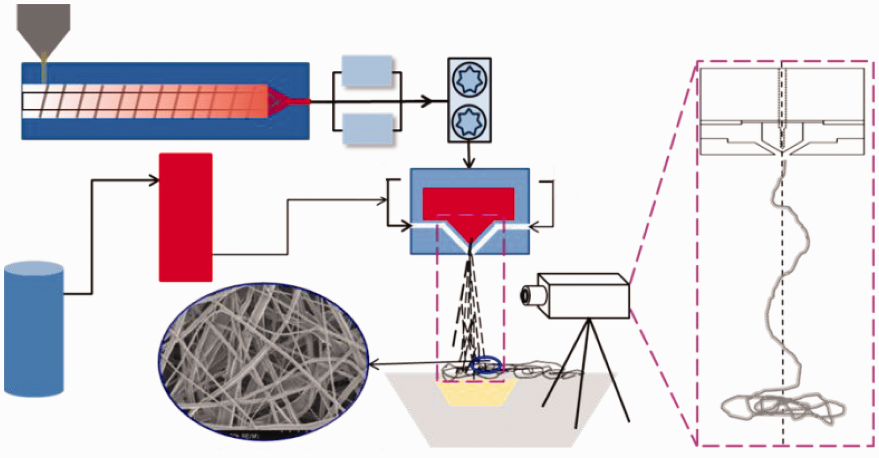
Schematic of melt-blowing process and fiber motion measuring system.

Airflow field simulation

Figure 2 shows the configurations and boundary conditions for the melt-blowing die. The molten polymer is extruded from the spinneret of the die, and the high-temperature and high-speed air-jet under the die will work on it. The air drag force applied on the polymer by the high-velocity airflow rapidly attenuates the fiber diameter to micrometer or finer size. The fiber formation is critically dependent on the aerodynamics of this process. The drag force due to the high-velocity air jet is the main cause of fiber attenuation in the melt-blowing process. Figure 2 shows the computational domain used in the simulations. The melt-blowing die is a slot die with a slot width of a = 1.05 mm, slot angle of α = 30, and nose piece width of f = 2 mm. The air flow entering the computational domain was set as a pressure inlet boundary condition at T = 537 K and P = 1.3 atm. The right boundary and the bottom boundary were set as pressure outlets with ambient air conditions (T = 300 K and P = 1atm). The left boundary was set as a line of symmetry. All other boundaries were assigned the default setting of being a wall at a temperature equal to 537 K. The computational domain below the die head was 100 mm × 40 mm. The computational domains of the die configurations are generated using GAMBIT 2.2.6. A quadrilateral structural grid was generated in the simulation area. Close to the symmetry line and the die face, the grid of this area is meshed to fine structure. The number of quadrilateral cells is about 14,000 in the simulation area.

Figure 2.

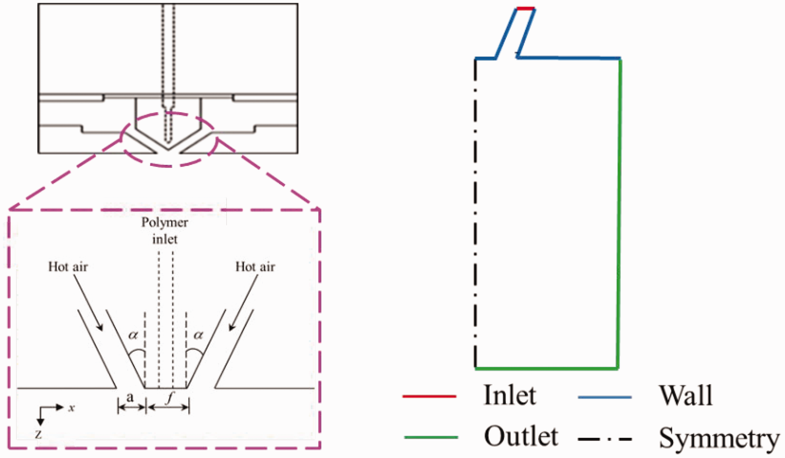
The configurations and boundary conditions for the melt-blowing die.

An ideal gas model and the k-ε turbulence model were used in this simulation.^17,25 The k-ε model is expressed as follows:

\frac{\partial (ρ k)}{\partial t} + \frac{\partial (ρ k u_{i})}{\partial x_{i}} = \frac{\partial}{\partial x_{j}} [(μ + \frac{μ_{t}}{σ_{k}}) \frac{\partial k}{\partial x_{j}}] + 2 u_{t} (\frac{\partial u_{i}}{\partial x_{j}} + \frac{\partial u_{j}}{\partial x_{i}}) \frac{\partial u_{i}}{\partial x_{j}} - 2 ρ ε M_{t}^{2}

(1)

\frac{\partial (ρ ε)}{\partial t} + \frac{\partial (ρ ε u_{i})}{\partial x_{i}} = \frac{\partial}{\partial x_{j}} [(μ + \frac{μ_{t}}{σ_{ε}}) \frac{\partial ε}{\partial x_{j}}] + 2 C_{ε 1} \frac{ε}{k} μ_{t} (\frac{\partial u_{i}}{\partial x_{j}} + \frac{\partial u_{j}}{\partial x_{i}}) \frac{\partial u_{i}}{\partial x_{j}} - 2 C_{ε 2} ρ ε (\frac{ε}{k} + 1)

(2)

G_{k} = - ρ u_{i}^{'} u_{j}^{'} \frac{\partial u_{i}}{\partial x_{i}}

(3)

u_{t} = ρ C_{μ} \frac{k^{2}}{ε}

(4)

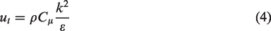
Equation (1) represents the kinetic energy; the right side of equation (1) represents the production of kinetic and the transformation of kinetic energy. Equation (2) is the turbulence dissipation rate. Equation (3) is used to calculate the generation of turbulence kinetic energy. Equation (4) is used to calculate the turbulent viscosity. In these equations, the values of the empirical constant are given as the following, $C_{ε 1} =$ 1.44, $C_{ε 2}$ = 1.92, $C_{μ} =$ 0.09, $σ_{k} =$ 1.0, $σ_{ε} =$ 1.3.

Melt-blowing fiber model

The bead–viscoelastic element model is used to simulate the fiber and study the fiber formation in melt-blowing process. A mixed Euler–Lagrange approach was adopted to derive the governing equations for modeling the fiber motion as it is being formed below the melt-blowing die. The polymer jet is extruded from the spinneret to form the fiber. The fiber is composed of a series of beads connected by the springs and dashpots viscoelastic elements. Figure 3 shows the schematic of a bead–viscoelastic element fiber model in this study.

Figure 3.

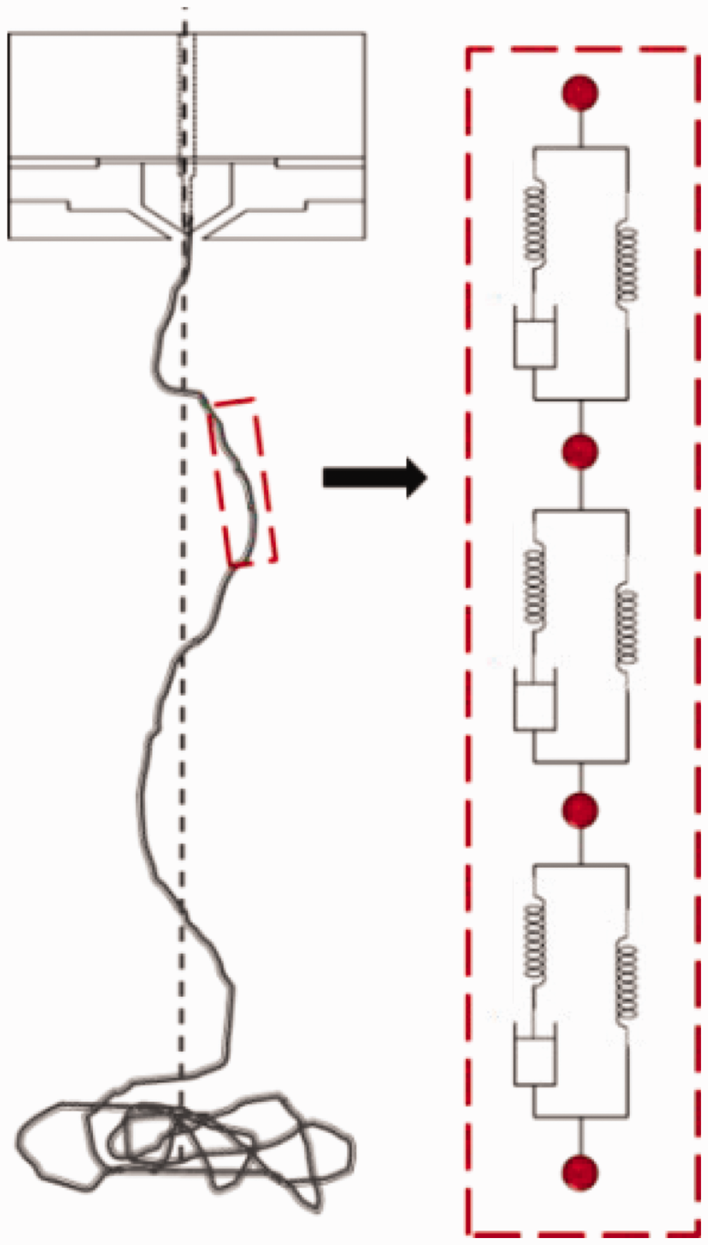
Schematic of a bead–viscoelastic element model for melt-blowing fiber.

The length of the fiber is determined by the coordinate position of the adjacent beads. The mass of the fiber is assigned to the beads in this model. For example, the bead i and a pair of adjacent beads, i + 1, form the fiber element (i, i + 1) and the length of element is given by

L_{i, i + 1} = [{(x_{i + 1} - x_{i})}^{2} + {(y_{i + 1} - y_{i})}^{2} + {(z_{i + 1} - z_{i})}^{2}]

(5)

The bead i mass is defined as m_i, as the contribution from its adjacent fiber elements (i − 1, i) and elements (i, i + 1). It can be described as follows

m_{i} = \frac{1}{2} ρ_{f} (A_{i - 1, i} l_{i - 1, i} + A_{i, i + 1} l_{i, i + 1})

(6)

where ρ_f is the fiber (polymer) density, A_i_-1, _i and A_i_, _i ₊₁ are the fiber cross-sectional areas of fiber elements (i − 1, i) and (i, i + 1), respectively, and are described as

A_{i - 1, i} = \frac{1}{4} π d_{i - 1, i}^{2}

(7)

A_{i - 1, i} = \frac{1}{4} π d_{i, i + 1}^{2}

(8)

where d_i_− 1, _i and d_i_, _i ₊₁ are the diameters of fiber elements (i − 1, i) and (i, i + 1), respectively.

The standard linear solid (SLS) model is used to express the polymer viscoelastic property. The fiber element consists of two Hookean springs and a dashpot. The governing constitutive equation is

\frac{(E_{1} + E_{2}) η}{E_{2}} \frac{d ε}{d t} + E_{1} ε = \frac{η}{E_{2}} \frac{d σ}{d t} + σ

(9)

where E₁, E₂ is the elastic modulus and η is the viscosity.

In the fiber formation process, the polymer jet is extruded from the spinneret and affected by the air flow immediately. The fiber movement is subjected to the air drag force, the viscoelastic force, the surface tension force, and the gravitational force.³⁶

For the fiber element (i − 1, i) and (i, i + 1), the air drag force F _di can be calculated by

F_{d i} = \frac{1}{2} (F_{d i - 1, i} + F_{d i, i + 1}) = \frac{1}{2} (F_{f i - 1, i} + F_{p i - 1, i} + F_{f i, i + 1} + F_{p i, i + 1})

(10)

In the melt-blowing process, the air drag force is composed of the parallel drag force F _f (friction drag) and the normal drag force F _p (pressure drag). The friction drag force and the pressure drag force can be expressed as³⁷

F_{f i - 1, i} = \frac{1}{2} C_{f} ρ_{a} v_{rti}^{2} π d_{i - 1, i} l_{i - 1, i}

(11a)

F_{f i, i + 1} = \frac{1}{2} C_{f} ρ_{a} v_{rti}^{2} π d_{i, i + 1} l_{i, i + 1}

(11b)

F_{p i - 1, i} = \frac{1}{2} C_{p} ρ_{a} v_{rni}^{2} π d_{i - 1, i} l_{i - 1, i}

(11c)

F_{p i, i + 1} = \frac{1}{2} C_{p} ρ_{a} v_{rni}^{2} π d_{i, i + 1} l_{i, i + 1}

(11d)

C _f is the friction drag coefficient and C _p is the pressure drag coefficient. $ρ_{a}$ is the air density. v_rti and v_rni are the relative velocities in parallel and normal to the direction of the fiber element at the bead i.

In Matsui’s studies,³⁸ C _f and C _p are given as

C_{f} = 0.78 {R e}_{f}^{- 0.61}

(12)

C_{p} = 6.96 {R e}_{n}^{- 0.440} {(\frac{d}{7.8 \times 10^{- 5}})}^{0.404}

(13)

The Reynold Re _f and Re _n are defined as

{R e}_{f} = \frac{ρ_{a} v_{rti} d}{μ_{a}}

(14)

{R e}_{n} = \frac{ρ_{a} v_{rni} d}{μ_{a}}

(15)

$μ_{a}$ is the air dynamic viscosity.

In equation (9), the tensile stress $σ_{i - 1, i}$ acting on the fiber element (i − 1, i), is given as

\frac{(E_{1} + E_{2}) η}{E_{2}} \frac{d l_{i - 1, i}}{d t} + E_{1} l_{i - 1, i} = \frac{η}{E_{2}} \frac{d σ_{i - 1, i}}{d t} + σ_{i - 1, i}

(16)

The adjacent beads’ viscoelastic force on the bead i, F _vei , is given as

F_{vei} = \frac{π d_{i, i + 1}^{2}}{4} σ_{i, i + 1} [\frac{x_{i + 1} - x_{i}}{l_{i, i + 1}} i + \frac{y_{i + 1} - y_{i}}{l_{i, i + 1}} j + \frac{z_{i + 1} - z_{i}}{l_{i, i + 1}} k] - \frac{π d_{i - 1, i}^{2}}{4} σ_{i - 1, i} [\frac{x_{i} - x_{i - 1}}{l_{i - 1, i}} i + \frac{y_{i} - y_{i - 1}}{l_{i - 1, i}} j + \frac{z_{i} - z_{i - 1}}{l_{i - 1, i}} k]

(17)

where

r_{i} = i x_{i} + j y_{i} + k z_{i}

is the bead i position in the xyz coordinate system.

Surface tension force restores the bent portion of the fiber to a straight shape fiber and acting on the bead i. It can be calculated by the fiber elements (i − 1, i) and (i, i + 1) and given as

F_{b i} = \frac{λ π {(\frac{d_{i - 1, i} {+ d}_{i, i + 1}}{2})}^{2} k_{i}}{4 {(x_{i}^{2} + y_{i}^{2})}^{1 / 2}} [{i x}_{i} {+ j y}_{i}]

(18)

$λ$ is the surface tension coefficient, k_i is the fiber part curvature.

Therefore, the force balance equation for bead i can be expressed as

m_{i} a_{i} = \frac{d^{2} r_{i}}{d t^{2}} = F_{f i} + F_{p i} + F_{vei} + F_{b i} + m_{i} g

(19)

In the melt-blowing process, there is a heat transfer between the fiber and airflow field. The energy equation is given as

m_{i} C_{i} \frac{d T_{i}}{d t} = - h π \frac{d_{i - 1, i} + d_{i, i + 1}}{2} \frac{l_{i - 1, i} + l_{i, i + 1}}{2} (T_{i} - T_{a i})

(20)

In equation (20), C_i is the fiber heat capacity, T_i is the temperature of fiber bead i, T_ai is the air temperature at bead i, and h is the convective heat transfer coefficient.

The three-dimensional fiber whipping motion is also studied in this model. The polymer melt introduces a time-dependent initial perturbation as it leaves the die, as shown in Equation 21.

x = a_{0} \sin (ω t)

(21a)

y = a_{0} \cos (ω t)

(21b)

In equation (21), a₀ is the initial perturbation amplitude, and $ω$ is the perturbation frequency.

Model solution procedure

(1) At the beginning of modeling, the fiber segment is formed by two beads 1 and 2. Bead 2 is near the die spinneret. The fiber segment length is first set to 0.5 mm, which equals the initial straight part. Initial physical properties are given to the two beads, including density, mass, diameter, and so on.

(2) As the procedure runs, beads in the system are driven by the air drag and gravity, which is calculated, based on the equations (10) to (21) and the velocity distribution of the airflow field mentioned in the results of simulation. The computer records the spatial position of beads at every time step.

(3) If the vertical distance between bead i + 1 and the orifice is larger than L (L is an independent variable), then a new bead (bead i + 2) will appear at the position of the orifice. The initial physical properties are also given to bead i + 2.

With iterations including the above procedure from the second to the third steps, we can follow the positions of all beads and obtain the path of the fiber motion in evolutionary time.

Results and discussion

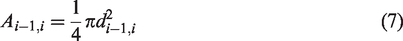
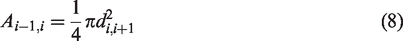
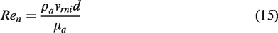
Figure 4 is the characteristic of the velocity distribution in the melt-blowing airflow field. Figure 4(a) shows the mean air velocity contour maps for the air flow field of the melt-blowing die. The velocity of the airflow steadily decreases as the distance from the die increases. The velocity flow field at distances close to the die is shown in Figure 4(b). As shown in Figure 4(b), there are two recirculation areas that occur in a triangular space located within a few millimeters of the center of the die. This zone is a velocity recirculation zone, where the velocities are relatively low and distribute between 0–50m/s. The eddy of the recirculation zones is important for rapid fiber attenuation and plays a significant role in fiber motion and fiber formation.

Figure 4.

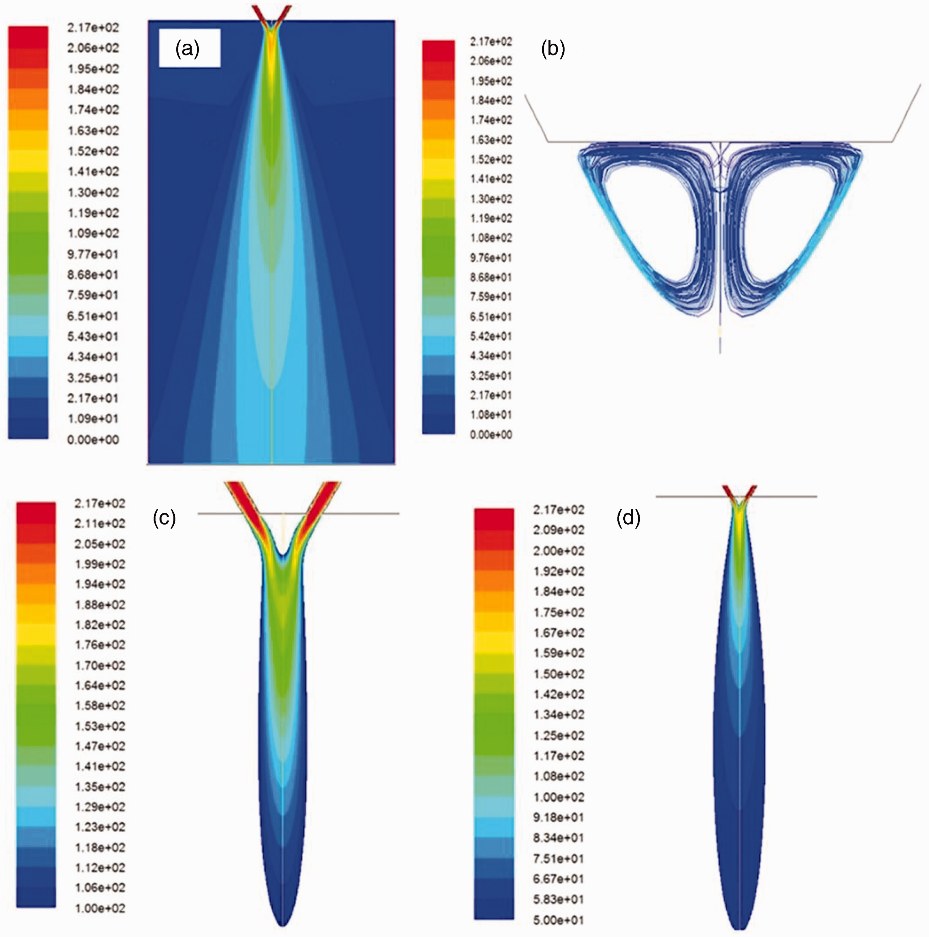
The result of simulation for the melt-blowing airflow field. (a)The velocity contour distribution for the melt-blowing die, (b) the velocity of airflow field close to the die heads; (c) the velocity distribution for 100 m/s–217 m/s in the melt-blowing process and (d) the velocity distribution for 50 m/s–217 m/s in the melt-blowing process.

Figure 4(c) shows the air velocity distributed between about 100–200 m/s. It is observed that the two separate jets combine at a position about 3 mm below the die face. The existence of eddy of the recirculation zones close to the die plate can cause the jet to deflect towards the downstream in the converging region. The two air jets eventually merge together at the point which is defined as the impingement point. It should be noted that the merging of the air jets produces high velocity and results in a rapid attenuation of the fiber. The interaction of the two air jets is manifested by the generation of high Reynolds stresses which lead to the fiber perturbation within this area. After the merging region, the air jets are in the fully combined region. Figure 4(d) shows that the velocities decay rapidly until they gradually become steady in this area. The velocity drop in this region is also believed to be the driving force for attenuation of the polymer melt and fiber formation in the melt-blowing process.

Figure 5 shows the motion trajectory of the polymer jet (fibers) at different times during the melt-blowing process. Figure 5(a) shows the fiber motion at the beginning stage. At the initial moment, the airflow velocity is low and the polymer jet has little whipping motion near the melt-blowing die. The fiber stays nearly parallel to the air stream and moves slowly. The polymer jet starts whipping after entering the two recirculation areas. The fluctuation amplitude is about 2 mm in the near field (0 mm < z < 5 mm). With increasing time, the polymer jet is continuously moving, the whipping of the polymer jet (fiber) starts to increase, and the motion trajectory becomes more complex, as shown in Figure 5(b). It can be seen clearly that the fiber whipping arises as soon as the fiber leaves the recirculation areas in Figure 5(b). It was pointed out that whipping motion could be associated with the change of air velocity, which caused the fiber movement to become more violent under the melt-blowing die. Whipping in the melt-blowing process is an aerodynamics-driven bending instability. The fiber is in the airflow field and one end of the fiber is not held in the movement process. The whipping of fiber is an aerodynamically driven bending instability in the melt-blowing process. Entov and Yarin³⁹ demonstrated that there is a critical velocity for the theory of aerodynamically driven jet bending. When the air velocity acting on the polymer jet exceeds the critical velocity, small disturbance of the jet will increase and develop into bending instability. The polymer jet exiting from the die spinneret meets with the high-velocity air at the air impinging point and becomes whipping since the airflow velocity fluctuates. In the impinging area (1 cm < z < 5 cm), the relative velocity between fibers and airflow increases due to the confluence of airflow, and the melt-blowing fibers are drawn increasingly. At the same time, the melt-blowing fibers are in a higher temperature field and the polymer has a better fluidity. The airflow velocity, polymer temperature, and polymer fluidity are affecting the fiber attenuation in this zone, which is the most important factor for the melt-blowing fiber spinning and formation. In this region, the melt fines are rapidly elongated and thinned with the velocity rising rapidly and the velocity gradient increasing. Figure 5(c) shows that the polymer jet continues to move forward, the velocity gradient between the polymer jet and air significantly decreases, the fiber stops drawing at the stop-point which the air velocity, and the fiber velocity become equal. It can be seen that the latter loop sometimes overruns the former one in the fiber motion trajectory. It indicates the whipping fluctuations move the fiber jet not only downwards but also upwards such that the fiber curve creates loops. This phenomenon is captured by the high-speed camera.

Figure 5.

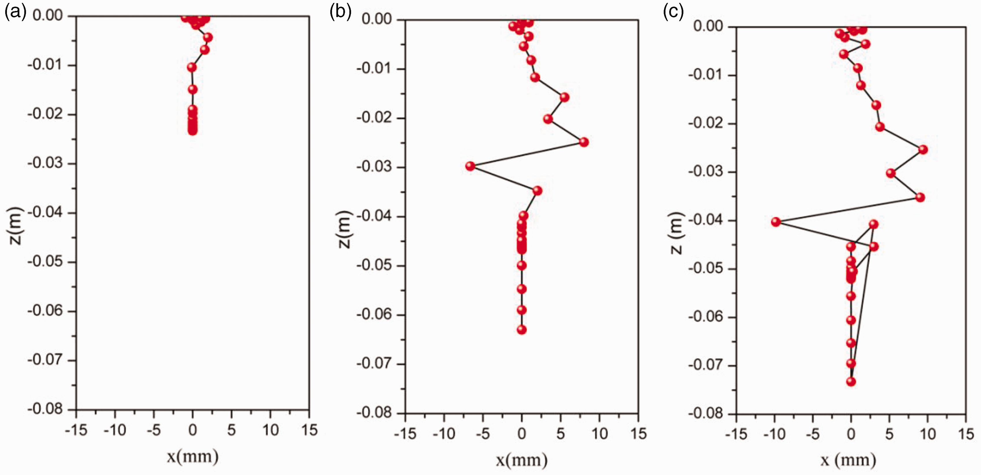
The time evolution of fiber whipping development for the simulation of melt-blowing. (a) t = 0.05 s, (b) 0.08 s and (c) 0.1 s.

Figure 6 shows the relationship between the airflow field and the fiber drawing ratio in the melt-blowing process. Figure 6(a) shows the simulation of melt-blowing airflow field. This result meets the description of Shambaugh’s work in which the melt-blowing process was separated into three regions.⁴⁰ Region I is the low-air-velocity region, where the path and time-independent fiber motion are similar to that in melt spinning. In Region II, the increase in air velocity causes fiber vibrations and subsequently breakage, thereby forming fiber segments. In Region III, the fiber experiences severe vibrations. The airflow patterns of melt-blowing die jets are shown schematically in Figure 6(b). The region extends a distance on each side of the airflow jet centerline and the airflow field can be characterized by three regions. Similar to the airflow field of the two parallel jets, a sub-atmospheric pressure zone close to the die plate causes the individual jets to curve towards each other in a region close to the die plate known as the converging region (Region I) and merge together at some downstream distance, known as the merging point. Downstream from the merging point in the merging region, the two jets continue to interact with each other up to the combined point where the mean air velocity on the centerline attains its maximum value (Region II). Downstream from the combined point, in the combined region, the two jets combine to form a single jet flow (Region III).

Figure 6.

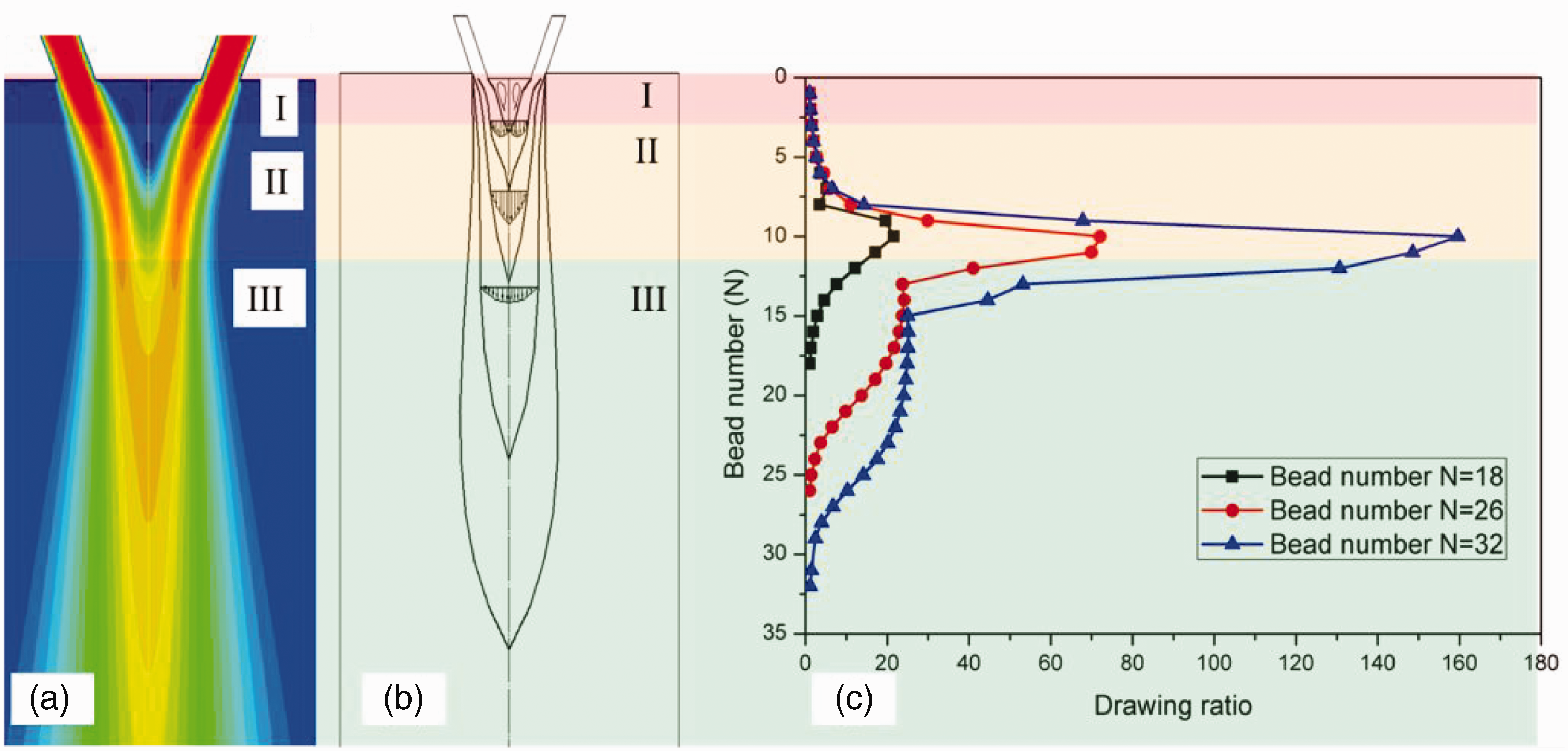
The relationship between the airflow field and the fiber drawing ratio: (a) the simulation of melt-blowing airflow field, (b) the schematic diagram of an air flow jet and (c) the drawing ratio of fiber in the melt-blowing process.

As mentioned, the air velocity distribution plays a significant role because polymer streams spend most of the time in the centerline below the die face. The polymer jet in the different regions obtains the different drawing ratios. The draw ratio is calculated by equation (22).

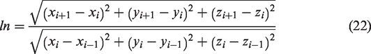
l n = \frac{\sqrt{{(x_{i + 1} - x_{i})}^{2} + {(y_{i + 1} - y_{i})}^{2} + {(z_{i + 1} - z_{i})}^{2}}}{\sqrt{{(x_{i} - x_{i - 1})}^{2} + {(y_{i} - y_{i - 1})}^{2} + {(z_{i} - z_{i - 1})}^{2}}}

(22)

Figure 6(c) illustrates the development of the fiber draw ratio for the model with different beads. In Region I, the mean air velocity on the centerline is negative in the recirculation zone. The fiber has a small draw in this region. The fiber draw ratio increases rapidly in Region II where the centerline velocity increases quickly. The peak of the fiber draw ratio corresponds to the location where the merging occurs in this region. The reason is that the velocity gradient between fibers and airflow increases due to the increase of airflow velocity. The air velocity increases to a maximum in this region. Figure 7 illustrated that rapid fiber attenuation occurs in the region and the motion trajectory of the fiber has large displacement. In Region III, the two air jets combine together to resemble single free jet flow behavior. The velocity gradient between air and fiber decreases in the area since the centerline air velocity drops rapidly. The draw ratio of the fiber begins to decrease in the zone.

Figure 7.

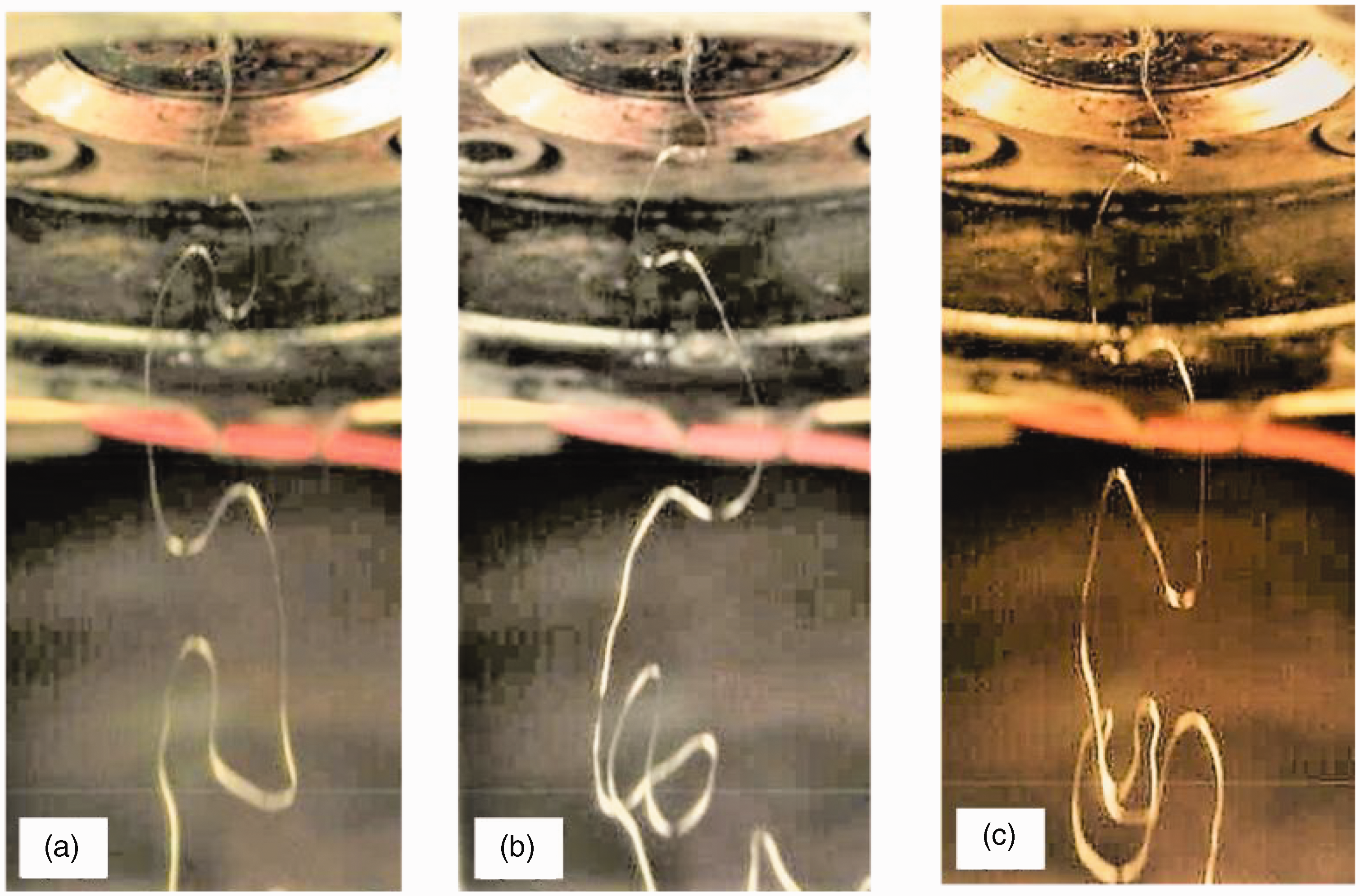
Evolution of fiber paths in the melt-blowing process, the time interval between the adjacent path profiles was 2 ms.

Figure 7 shows the time evolution of fiber motion by high-speed camera in the melt-blowing process. It appears that there are three different regions for the fiber attenuation. This is consistent with the simulation result of airflow field and fiber motion. At the beginning, it is the low air velocity region where the fiber stays nearly parallel to the air stream. This distance is short and then fiber moves into the air recirculation areas. It can be seen that fiber bending instability occurs as soon as the polymer jet enters the recirculation areas. Figure 7(a) demonstrates a short distance straight movement for the polymer jet. After that, the polymer jet develops a bending, spiraling, and looping path. The loops of polymer jet will grow longer and thinner as the perimeter of the loop increases. The reason is that the two air jets are converging in the merging region. The mean velocity of airflow exhibits maxima value and there is no inner region with recirculation in this zone. The relative velocity difference between fibers and airflow increases due to the sharp increase in airflow velocity and the melt-blowing fibers are drawn and refined. It is noted that this region is the most important for the melt-blowing fiber formation. During airflow velocity decay, Figures 7(b) and 7(c) show that the latter loop of the fiber overruns the former loop of the fiber. The adjacent loops can entangle as they move down a certain distance. During the movement, the fibers are draw by the airflow and the loop perimeter of fiber increases with increasing distance from the die. When the fiber loops are far away from the spinneret, fiber loops expand to a three-dimensional structure due to the entanglements. According to Wieland’s study,⁴¹ high aerodynamic forces act on the fiber loops due to high relative velocity gradients causing the fiber to elongate. However, the disturbance shape for most of the time before overturning is weakly dependent upon the drag and is mainly determined by the ‘lift’ component of the aerodynamic force. Zeng mentioned the loop perimeter as a function of the distance of collector from the die. As the perimeter of the loop increases, the diameter of the fiber becomes smaller.⁴²

To further understand the fiber formation and attenuation in the melt-blowing process, the resultant fiber diameters are measured at positions of 10 mm, 50 mm, 80 mm, and 100 mm below the die. Figure 8 shows the scanning electron microscope (SEM) images of the melt-blown fibers. There are different junctions in the melt-blowing fiber web. For the short distance (z = 10 mm), the fibers can stick together where fibers have not yet cooled as soon as the continuous polymer jets leave the spinnerets. The interlacing also can happen between two or among several fibers due to the randomly motion of fibers. The average diameter of the fiber was measured as 43.98 µm, 6.73 µm, 4.36 µm, and 3.38 µm at distances of 1 cm, 5 cm, 8cm, and 10 cm, respectively. For the 0.5 mm (500 µm) initial fiber diameter, the whole diameter reduction ratio can be calculated as 147.93. Therefore, the main diameter reduction ratio contributed by the distance from z = 50 mm is about 50.22% of the whole diameter reduction ratio. From Figure 5 and Figure 6, the main whipping in the melt-blowing process appears at a distance between1 cm and 5 cm; it can be seen that whipping plays a role in fiber attenuation. The results also support the known investigation that the fiber attenuation mostly occurs in the region when the distance from the die is within 5 cm.⁴⁰

Figure 8.

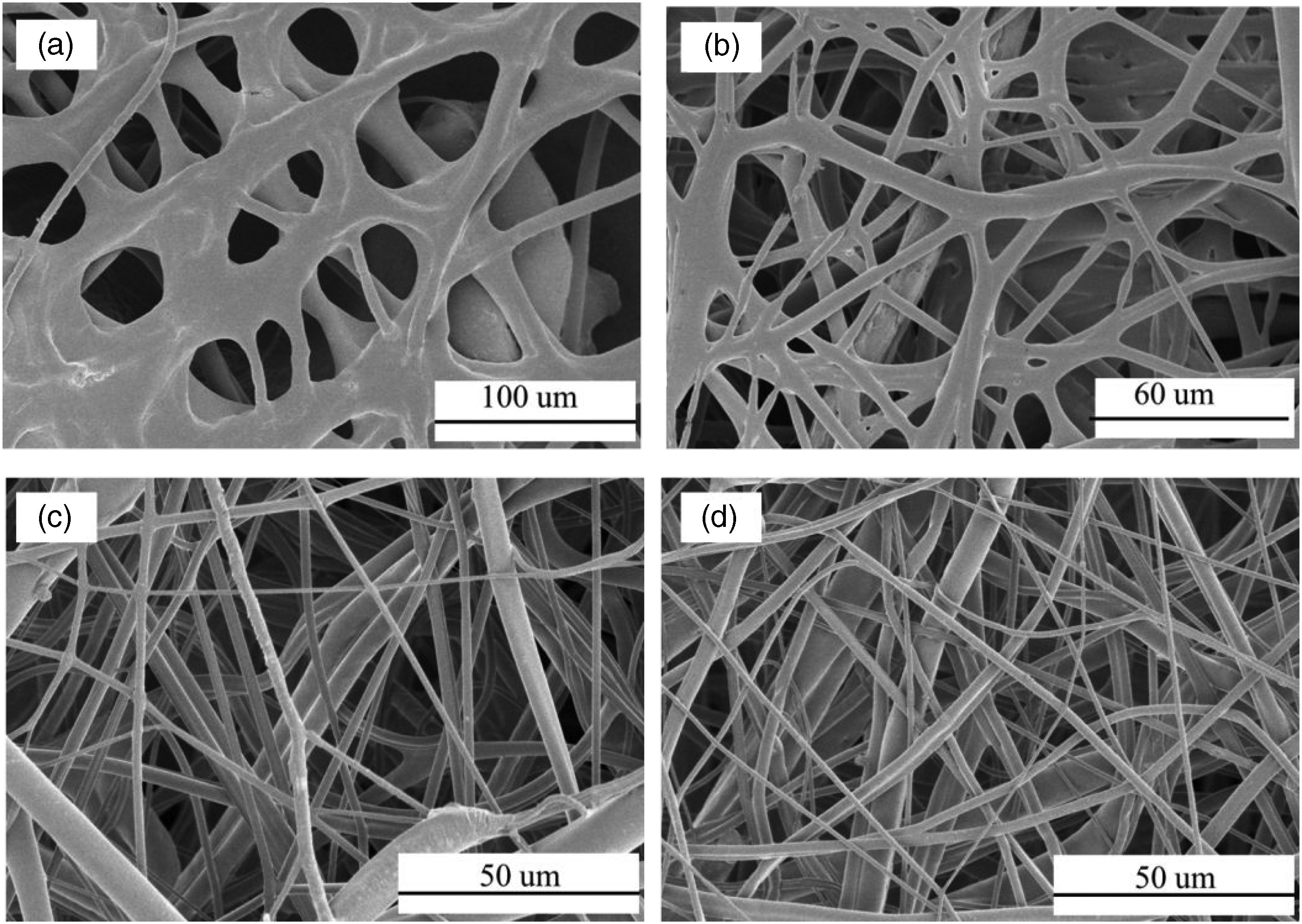
The morphology of fibers produced by the melt-blowing process at (a) z = 10 mm, (b) z = 50 mm, (c) z = 80 mm and (d) z = 100 mm, respectively.

Conclusion

In this work, the airflow field distribution for the slot-die melt-blowing process was simulated and analyzed to reveal the effects of the fiber motion and attenuation. A bead–viscoelastic element model was applied to simulate the fiber motion in melt-blowing process. The dynamic movement of fiber was captured by a high-speed camera in a short distance. There were three regions in the airflow field of melt-blowing process for fiber attenuation. The polymer jet starts whipping after entering the two recirculation areas in Region I. The main attenuation for fiber was in Region II where the relative velocity between fibers and airflow increases due to the confluence of airflow. The relationship between the airflow field distribution and the fiber attenuation has been discussed with the fiber simulation model and through experiment. The simulation results of fiber motion and attenuation are consistent with the experimental observations. This work firstly explains the conclusion by demonstrating the relationship among the airflow, fiber whipping, and the fiber attenuation, which is useful information for the melt-blowing fiber formation.

Footnotes

Declaration of conflicting interests

The author(s) declared no potential conflicts of interest with respect to the research, authorship, and/or publication of this article.

Funding

The author(s) disclosed receipt of the following financial support for the research, authorship, and/or publication of this article. This research is supported by Zhejiang Provincial Natural Science Foundation of China (LY22E060005), Jiaxing Science and Technology Project (2022AY10023), Key Laboratory of Yarn Materials Forming and Composite Processing Technology of Zhejiang Province (MTC-2022-08), National Natural Science Foundation of China (52263002).

ORCID iDs

Han Wanli

Yudong Wang

Xinhou Wang

References

Ramakrishna

Fujihara

Teo

W E

, et al. An introduction to electrospinning and nanofibers. Singapore: World Scientific Publishing, 2005, pp. 135–142.

Drabek

Zatloukal

Meltblown technology for production of polymeric microfibers/nanofibers: A review. Phys Fluids 2019; 31(9): 91301–91326.

Luiso

Henry

J J

Pourdeyhimi

, et al. Meltblown polyvinylidene difluoride as a Li-ion battery separator. ACS Appl Poly Mater 2021; 3(6): 3038–3048.

Kenry, Lim

C T.

Nanofiber technology: current status and emerging developments. Prog Polym Scie 2017; 70: 1–17.

Chen

Tung

One-step electrospinning to produce nonsolvent-induced macroporous fibers with ultrahigh oil adsorption capability.

Macromolecules 2017; 50(6): 2528–2534.

Salehhudin

Mohamad

Mahadi

WNL

, et al. Multiple-jet electrospinning methods for nanofiber processing: A review. Mater Mfg Proc 2018; 33(5): 479–498

Han

Nurwaha

, et al. Free surface electrospun fibers: The combined effect of processing parameters. Polym Engng Sci 2014; 54(1): 189–197.

Fedorova

Pourdeyhimi

High strength nylon micro- and nanofiber based nonwovens via spunbonding.

J Appl Polym Sci 2007, 104(5): 3434–3442.

Zhang

Peijs

, et al. Fabrication and properties of poly(tetrafluoroethylene) nanofibres via sea-island spinning. Polymer 2017; 109: 321–331.

10.

Wente

VA.

Superfine thermoplastic fibres.

Ind Engng Chem 1956; 48(8): 1342–1346.

11.

Ellison

Phatak

Giles

, et al. Melt blown nanofibers: Fiber diameter distributions and onset of fiber breakup. Polymer 2007; 48(11): 3306–3316.

12.

Uppal

Bhat

Eash

, et al. Meltblown nanofiber media for enhanced quality factor. Fibers Polym 2013; 14(4): 660–668.

13.

Hassan

Yeom

Wilkie

, et al. Fabrication of nanofiber meltblown membranes and their filtration proper-ties. J Membr Sci 2013; 427(0): 336–344.

14.

Han

Bhat

Wang

Investigation of nanofiber breakup in the melt-blowing process.

Ind Engng Chem Res 2016; 55(11): 3150–3156.

15.

Sun

Han

Wang

, et al. Overview of the fiber dynamics during melt blowing. Ind Engng Chem Res 2022; 61(2): 1004–1021.

16.

Barilovits

Khan

Shim

Experimental investigation of the fiber formation process and web structures using an annular meltblowing spinneret.

Ind Engng Chem Res 2021; 60(37): 13627–13636.

17.

Wang

Zhou

Experimental and numerical analysis of an improved melt-blowing slot-die. e-Polymers 2019; 19(1): 612–621.

18.

Soltani

Macosko

CW.

Influence of rheology and surface properties on morphology of nanofibers derived from is-lands-in-the-sea meltblown nonwovens.

Polymer 2018; 145: 21–30.

19.

Sun

Ruan

Wang

, et al. Numerical study of melt-blown fibrous web uniformity based on the fiber dynamics on a collector. Ind Engng Chem Res 2019; 58(51): 23519–23528.

20.

Sun

Yang

Sun

, et al. Simulation and modeling of microfibrous web formation in melt blowing. Ind Engng Chem Rese 2016; 55(18): 5431–5437.

21.

Han

Wang

Multi-objective optimization of the coat-hanger die for melt-blowing process.

Fiber Polym 2012; 13(5): 626–631.

22.

Han

Wang

Optimal geometry design of the coat-hanger die with uniform outlet velocity and minimal residence time.

J Appl Polym Sci 2012; 123(4): 2511–2516.

23.

Huang

Zeng

Effects of compatibilizer and airflow field on the formation of helical microfibers via melt blowing.

J Polym Sci. Part B: Polym Phys 2019; 57(21): 1423–1433.

24.

Xie

Han

Jiang

, et al. Turbulent air flow field in slot-die melt blowing for manufacturing microfibrous nonwoven materials. J Mater Sci 2018; 53(9): 6991–7003.

25.

Han

Xie

Shi

, et al. Study on airflow field and fiber motion with new melt blowing die. Polym Engng Sci 2019; 59(6): 1182–1189.

26.

Wang

Investigation on a new annular melt-blowing die using numerical simulation.

Ind Engng Chem Res 2013; 52(12): 4597–4605.

27.

Banerji

Jin

Mahanthappa

, et al. Porous fibers templated by melt blowing cocontinuous immiscible polymer blends. ACS Macro Lett 2021; 1196–1203.

28.

Luiso

Henry

Pourdeyhimi

, et al. Fabrication and characterization of meltblown poly(vinylidene difluoride) membranes. ACS Appl Polym Mater 2020; 2(7): 2849–2857.

29.

Sun

Song

, et al. Numerical modelling of microfibers formation and motion during melt blowing. J Text I 2018; 109(3): 300–306.

30.

Han

Wang

Modeling melt blowing fiber with different polymer constitutive equations.

Fibers Polym 2016; 17(1): 74–79.

31.

Hao

Zeng

A review on the studies of air flow field and fiber formation process during melt blowing.

Ind Engng Chem Res 2019; 58(27): 11624–11637.

32.

Rao

Shambaugh

RL.

Vibration and stability in the melt blowing process.

Ind Engng Chem Res 1993; 32(12): 3100–3111.

33.

Chhabra

Shambaugh

Experimental measurements of fiber threadline vibrations in the melt-blowing process.

Ind Engng Chem Res 1996; 35(11): 4366–4374.

34.

Beard

Shambaugh

, et al. Online measurement of fiber motion during melt blowing. Ind Engng Chem Res 2015; 46(22): 7340–7352.

35.

Xie

Zeng

Turbulent air flow field and fiber whipping motion in the melt blowing process: experimental study.

Ind Engng Chem Res 2012; 51(14): 5346–5352.

36.

Zeng

Sun

Wang

XH.

Numerical approach to modeling fiber motion during melt blowing.

J Appl Polym Sci 2011, 119(4):2112–2123.

37.

Sun

Song

, et al. Numerical modeling of microfibers formation and motion during melt blowing. J Text Inst 2018; 109(3): 300–306.

38.

Matsui

Air drag on a continuous filament in melt spinning.

Trans Soc Rheology 1976; 20(3): 465–473.

39.

Entov

Yarin

AL.

The dynamics of thin liquid jets in air.

J Fluid Mech 1984; 140: 91–111.

40.

Shambaugh

RL.

A macroscopic view of the melt-blowing process for producing microfibers.

Ind Engng Chem Res 1988; 27(12): 2363–2372.

41.

Wieland

Arne

Marheineke

, et al. Melt blowing of viscoelastic jets in turbulent airflows: Stochastic modeling and simulation. Appl Math Modell 2019; 76: 558–577.

42.

Xie

Zeng

Online measurement of fiber whipping in the melt-blowing process.

Ind Engng Chem Res 2013; 52(5): 2116–2122.