



Abstract
There is a complex interaction between primary fibers in pre-colored fiber blends, which leads to the impracticality of Duncan’s additive theory in the single-constant Kubelka–Munk (KM-1) model, resulting in poor accuracy for color prediction. This paper builds an optimized combined spectral calibration model based on the KM-1 function to solve this issue. This proposed model involves colored and non-colored parts with trained spectral coefficients, and was established to achieve a good matching between the predicted and actual ratio of the absorption coefficient K to the scattering coefficient S, K/S of samples for color prediction from the perspective of the spectrum. Experimentally, five primary cotton fibers were selected and prepared into fiber blends to demonstrate its validation, and its optimal number of training samples was found to be only 14, which was much less than the general training sampling method using half of all samples directly. Finally, a remarkable average color difference of only 0.63 CIEDE2000 units for 74 test specimens was achieved on this optimized model, which was significantly lower than that of the KM-1 model (∼1.16), two-constant KM model (∼1.03), Stearns–Noechel model (∼1.16) and Friele model (∼1.11). The results indicate that the optimized model behaves well and could be applied in the color prediction of pre-colored fiber blends.
Keywords
Pre-colored fiber blends are designed for multiple colors just through mixing only several primary fibers at different ratios.1,2 Compared with the traditional dyeing process, this production has the advantages of low water consumption, being environmentally friendly and having a unique visual haze effect and special beauty. Therefore, accurate color matching for it is one of the most important problems. It is fundamental to establish an effective and universally applicable model for color prediction and to describe the mechanism of color blending accurately.
Currently, several color prediction models for pre-colored fiber blends have been proposed and extensively studied, which were mainly based on empirical and theoretical models. In 1944, the Stearns–Noechel (S-N) model3,4 was proposed by Stearns and Noechel on the basis of the additive theory. The additive formula always needs a transfer function to satisfy the linear relationship, and the formula is as follows:
At present, these two empirical models have been applied to different fiber materials, yarns and fabrics.6–10 Studies on the S-N model and Friele model have been focused on the optimal empirical parameters to achieve accurate recipes for color prediction. Liu et al. 11 studied the optimal parameters of the S-N and Friele models for blending yarns by statistical analysis. It was found that the S-N model modified by components performed better for blends with components below five, and when this number reached five, the Friele model modified by the median should be applied. Li et al. 12 also proposed a spectrophotometric color matching algorithm based on the S-N model to improve the accuracy. In addition, Shen et al. 13 combined the S-N model with the artificial neural network (ANN) method to obtain a lower mean color difference of 0.86 CMC(2:1) units, which was better than both the ANN (2.21) and S-N (1.66) laws. However, the applicability and accuracy of the experimental models rely heavily on the number and categories of training samples. Moreover, their coefficients change not only with the categories, but also the differences in processing, testing conditions and other factors. 14 In this case, the theoretical models are more appealing.
The most common theoretical models are the single-constant and two-constant laws of the Kubelka–Munk (KM-1 and KM-2) theory, which was derived by Kubelka and Munk in 1931.15,16 For an infinitely thick and opaque material, the KM theory is formulated as follows:
In 1987, Walowit et al. 18 proposed a method of solving the absorption and scattering coefficients in the KM-2 model using the least-squares algorithm. Since then, the KM-2 model with the least-squares algorithm has been a very frequently used method in color prediction. This method has been applied in different kinds of fibers, yarns and fabrics.19–23 However, it is difficult to apply in practical cases because of its low prediction accuracy. Zhang et al.24,25 converted the Ki,λ of Equation (6) to (Ki,λ/Si,λ)*Si,λ to introduce Ki,λ/Si,λ of primary fibers in fiber blends based on the KM-2 law in color prediction, which improved the accuracy of the original model. Wang et al. 26 proposed an iteration method for the color prediction of stacked blending filaments. The predicted reflectance of a filament above the background was calculated by the KM law and set as the reflectance of background Rg for the next iterate. The parameters of the reflectance formula based on the KM law were the K and S of a monofilament from training mixed films on the KM-2 model and the reflectance of background Rg. The results showed that the average and maximum color differences obtained by the new model were 0.91 and 2 (CMC) (2:1) units, which were less than those of the KM theory (1.06 and 2.5).
The KM-1 model has the advantages of simple calculation and convenience in industry application, although it has commonly performed badly in past studies. 27 Some scholars have carried out to studies of performance and improvement strategies. Wei et al. 28 established a new additivity formula with a correction coefficient n based on the KM-1 method. This new formula effectively reduced the average color difference of 16 fabric in two-, three- and four-blends from 5.48 to 0.91 (CMC) (2:1) units. Nevertheless, their coefficient n trained by 10 specimens varied with the types and quantities of components in the samples. Gao et al. 29 adopted the min-max standard mapping method to eliminate the influence of extreme K/S values in the KM-1 model and determined the best optimal mapping range by the traversal algorithm for cotton fiber blends. However, for samples with white or black fibers, it was necessary to carry on this algorithm twice to ensure the mean color difference was below 1 (CMC) (2:1) units. Hence, the KM-1 model still needs an effective, convenient and widely used optimization method to improve its accuracy for color prediction in pre-colored fiber blends.
An optimized spectral correction model was proposed in this work to improve the color prediction of pre-colored cotton fiber blends based on the KM-1 model. It studied the interaction between fibers of the addition theorem from a new perspective of the spectrum on two parts of colored primary fibers and non-colored ones. Three-blends with colored fibers and two-blends with non-colored fibers were prepared as training samples, whose numbers were found to be nine and five, respectively. Finally, its accuracy turned out to be better than that of the S-N model, Friele model, KM-2 model and KM-1 model for 74 test samples.
Methods
As mentioned above, dye molecules are attached to the fibers, which make fibers possess different absorptions and scattering intensities on light. The fiber blend is a mixture of fibers with different colors, and its internal interaction is complex, making it difficult to reveal by a single linear relationship.
Different absorption and scattering properties of various colored fibers can cause inner multiple and complex light interactions. Theoretically, primary fibers in bicolor mixed assemblies selectively absorb and scatter lights, consisting of corresponding different absorption coefficients K and scattering coefficients S. However, the KM-1 model was established based on the assumption that the scattering coefficients S of primary fibers are the same and equal to those of blended mixtures, 27 excluding parts of the complicated scattering light interactions in fiber blends. Thus, this simplified linear additive model turns out to have relatively low accuracy in color prediction.
For the reason that the reflectance and K/S of the mixed fibers cannot be calculated by a single linear addition, an intermediate function should be proposed to consider the interaction in fiber blends and minimize the error between the theoretical and actual values. The function based on Equation (5) is as follows:
Experimental details
Materials and sample preparation
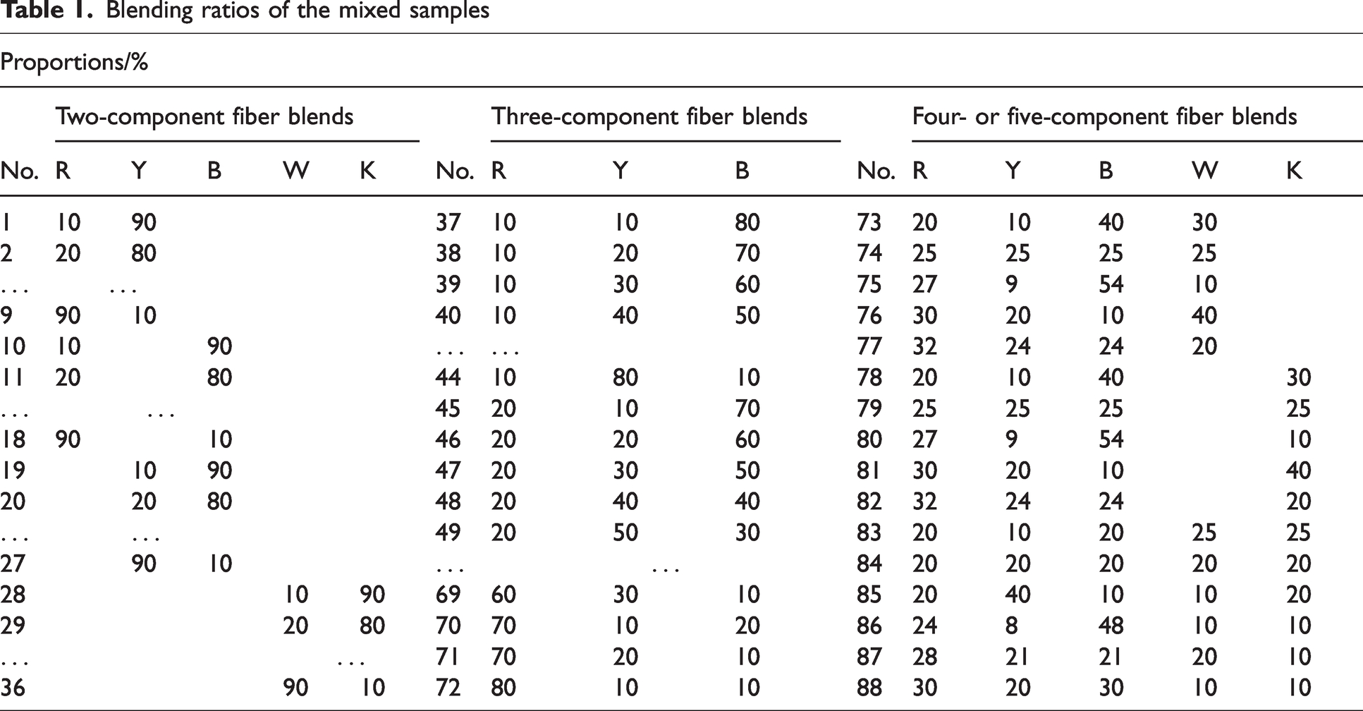
Three colored cotton fibers, comprising red (R), yellow (Y) and blue (B) fibers, and two non-colored cotton fibers, colored white (W) and black (K), were used as materials in this experiment. The reflectance, K/S spectra and images of these five primary fibers are shown in Figure 1. A total of 88 cotton fiber blending samples were prepared by mixing two (RY, YB, RB, WK), three (RYB), four (RYBW and RYBK) and five (RYBWK) kinds of cotton fiber slivers through a Y111 drafting instrument by simulating sliver blending at different ratios. In particular, two-blends and three-blends were mixed in fractional concentration increments of 10% for each, while four and five primary fibers were blended randomly; their specific ratios are listed in Table 1. Parts of the three colored cotton fibers blends (RYB) and non-colored fiber blends (WK) were adopted as training samples. These samples were designed to optimize the KM-1 model and determine the optimal number of training samples. The remaining samples were applied as testing samples to verify the effectiveness of the optimized model. Images of these samples were taken by a camera and are shown in Figure 2.
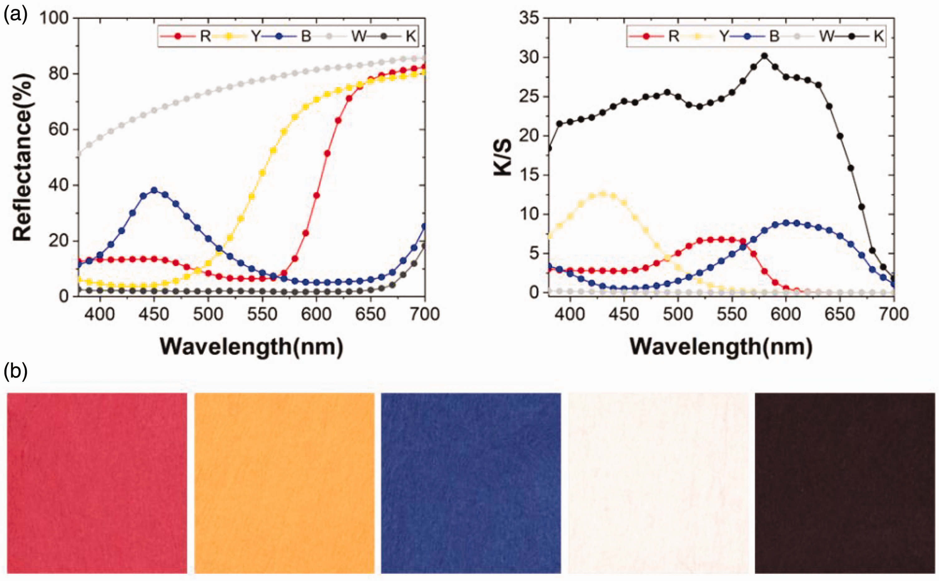
Five primary cotton fibers: (a) reflectance and K/S curve and (b) color images. R: red; Y: yellow; B: blue; W: white; K: black.
Blending ratios of the mixed samples
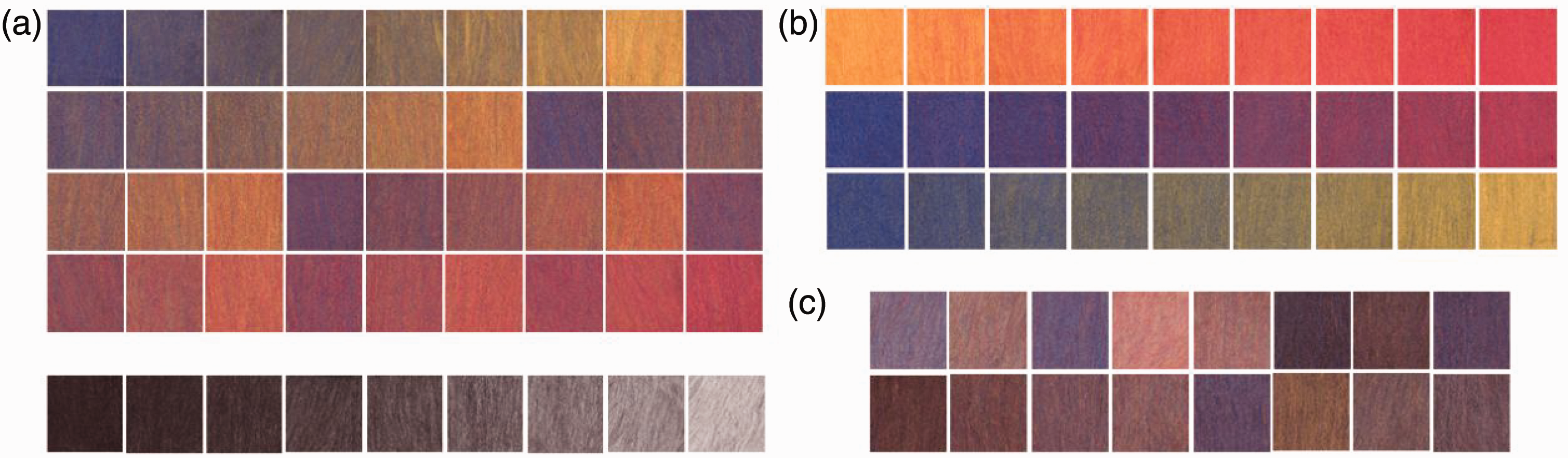
Images of fiber blending samples: (a) RYB fiber blends and WK fiber blends; (b) two-component fiber blends (RY, RB, YB) and (c) four- and five-component fiber blends (RYBW, RYBK, RYBWK). R: red; Y: yellow; B: blue; W: white; K: black.
Color measurement
Color measurement of the samples was carried out by Datacolor 600 spectrophotometer with the optical geometry of the d/8 system. To get reliable and repeatable color measurement data, each fiber sample with a weight of 4 g was loaded into a container with optical glass and squeezed until opaque, ensuring that the fibers were arranged in parallel. The measured values were recorded as 33-dimensional spectral reflectance data at intervals of 10 nm in the wavelength range (380–700 nm), and the specular component of the reflectance was included. To reduce the potential measurement error as much as possible, the largest aperture of 30 mm was selected to randomly measure nine times at different locations and directions over the whole surface of samples. Then the average of the nine measurements was taken as true color data of samples with paralleled fibers. In addition, the optical glass correction 30 was taken to eliminate the influence of the optical glass.
Optimized spectral calibration methods
Establishment of the optimized spectral calibration model
The prediction deviation of the KM-1 model mainly comes from the inapplicability of the addition theory. To improve its accuracy, nine non-colored fiber blends (WK) and 36 colored fiber blends (RYB) were adopted as the training materials here. Their (K/S)
mix,λ
based on the KM-1 model and their measured (K/S)
act,λ
based on Equation (4) were analyzed at each wavelength, respectively. Interestingly, obvious linear relationships between them were observed at each wavelength from 380 to 700 nm at an interval of 10 nm, as illustrated in Figure 3. In particular, the differences between them were probably due to the interaction between the primary fibers in the mixed samples and the simplified assumption. This assumption was that the scattering coefficient of the monochromatic fiber is about equal to that of the mixed fibers. Hereby, a linear equation was proposed based on Equation (7) in this paper aiming to reduce color differences, as follows:
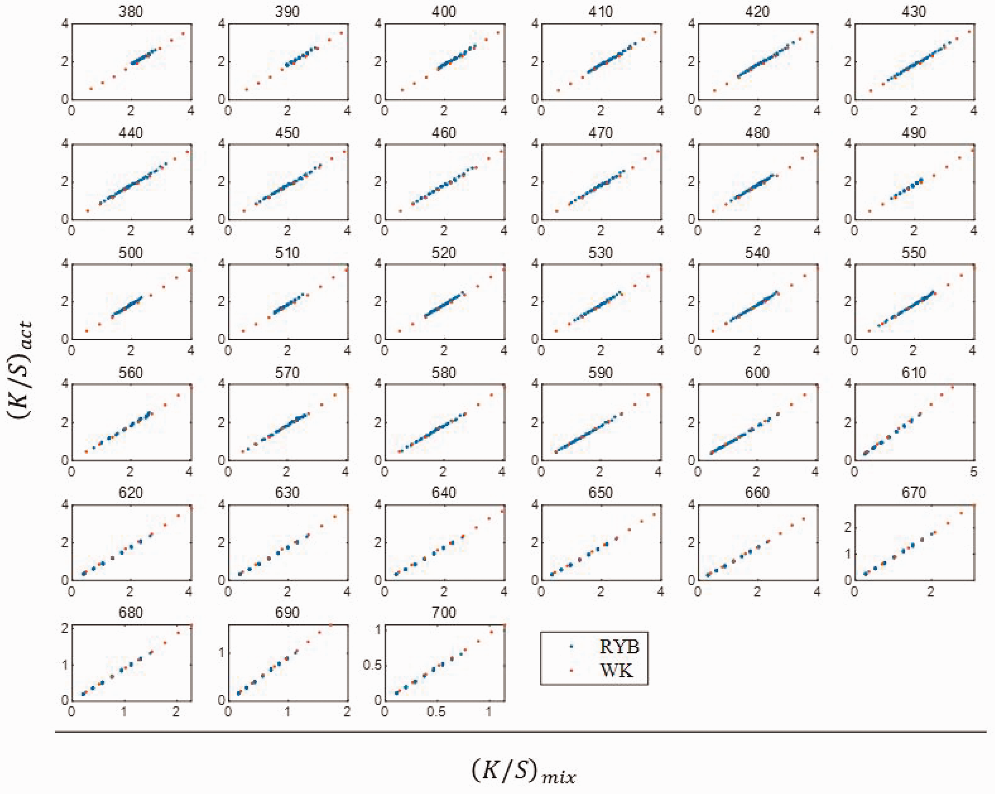
Comparison of (K/S) mix,λ and (K/S) act,λ at 33 spectral wavelengths of 36 RYB samples and nine WK samples. R: red; Y: yellow; B: blue; W: white; K: black.
As observed in Figure 3, although the RYB and WK samples shared a similar linear relationship, their linear inclinations were not consistent completely. In this case, they need to be explored separately. A combined spectral correction formula was formed with two parts of colored fiber blends and non-colored ones based on Equation (8):
Determination of the number of training samples
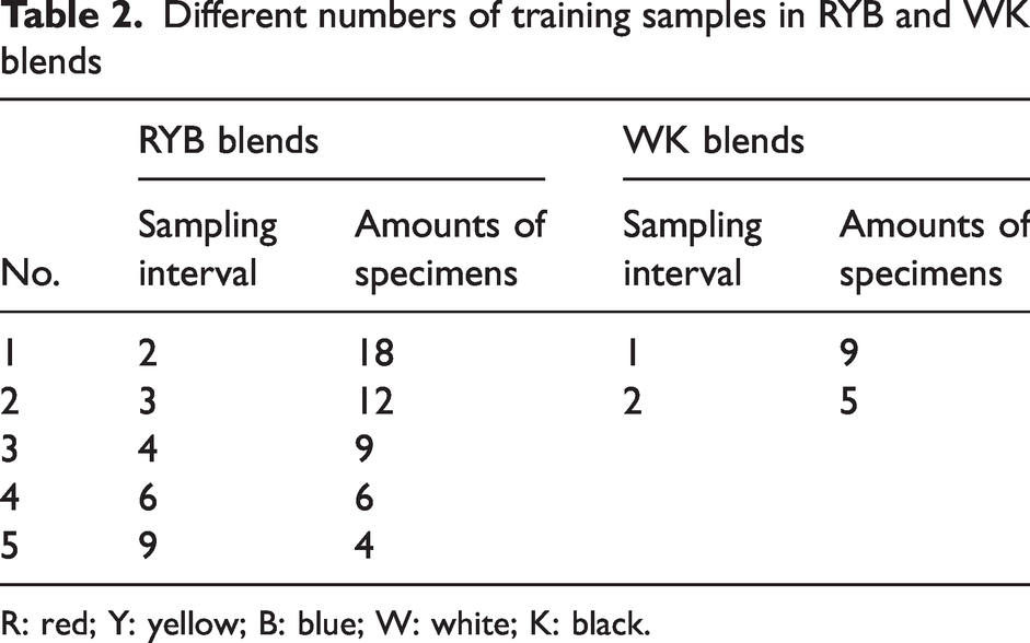
Usually, it is necessary to determine a certain number of training samples to reduce random error and ensure accuracy in the study of color prediction. For example, Zhang 31 declared 18 colored three-blends and nine non-colored fiber blends, white and black fibers, as training samples on the proposed KM-2 model, whose number was concluded to involve the range of fiber proportions as much as possible. Thus, to ensure the universality and justness of training samples, different sampling intervals of RYB and WK training samples were investigated as follows, referring to Table 2.
Different numbers of training samples in RYB and WK blends
R: red; Y: yellow; B: blue; W: white; K: black.
The correction spectral coefficients of Equation (8) could be obtained using the different schemes of training samples in Table 2 on the linear regression method. Afterwards, they were applied to calibrate the spectral predicted (K/S) mix,λ of 36 RYB and nine WK samples based on Equation (5), separately.
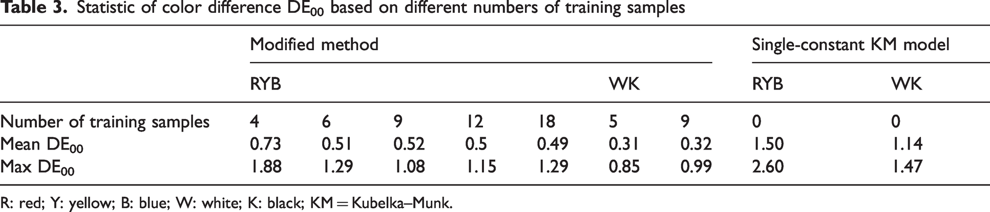
Color difference is the most important evaluation index, and the DE00 color difference formula 32 was used as the colorimetric metric. The values for the color difference formula were obtained under the CIE standard illuminant D65 and the 10° standard observer. For each sample, the predicted reflectance can be calculated from Equation (4). Meanwhile, the color information of each sample measured by a Datacolor 600 spectrophotometer was regarded as the standard, and the DE00 color difference between the predicted and measured values can be calculated. Then the color difference results based on this method were compared with those based on the KM-1 model using 36 RYB and nine WK specimens, respectively. For their specific color difference information, refer to Figure 4 and Table 3.
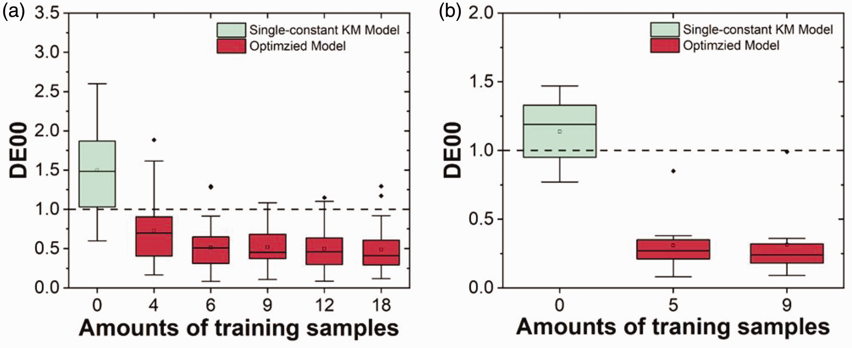
Comparison of color difference distribution based on the proposed method for different numbers of training samples and that of the single-constant Kubelka–Munk law: (a) RYB samples and (b) WK samples. R: red; Y: yellow; B: blue; W: white; K: black.
Statistic of color difference DE00 based on different numbers of training samples
R: red; Y: yellow; B: blue; W: white; K: black; KM = Kubelka–Munk.
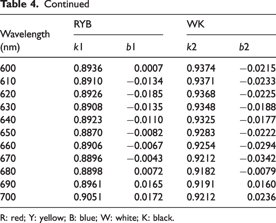
Figure 4 exhibits lower mean values and distribution ranges of DE00 based on the optimized method than those of the KM-1 model for both RYB and WK specimens, proving the sufficient stability and effectiveness. In particular, as shown in Table 3, the mean and maximum values of DE00 for RYB specimens drop as the number of their training samples increases, and then remain constant after this number reaches six. It is worth mentioning that the max DE00 for RYB specimens of 9, 12 and 18 training samples were all from the #46 sample, which was possibly caused by fiber loss and inhomogeneous mixing during sample preparation. Hence, although the accuracy of spectral correction increases as the number of training samples increases, an inaccurate sample may gain a larger DE00. In addition, these DE00 values based on five training samples in WK materials were even slightly smaller than those of nine samples. Accordingly, nine RYB and five WK samples were selected as training samples for the spectral correction of colored and non-colored fiber blends here, respectively. Their corresponding correction coefficients at each wavelength are listed in Table 4. The remaining 27 RYB and four WK specimens were adopted as part of the testing samples to examine the proposed model.
Correction coefficients for colored fiber blends and non-colored fiber blends
R: red; Y: yellow; B: blue; W: white; K: black.
Application and discussion
Prediction results for the optimized method
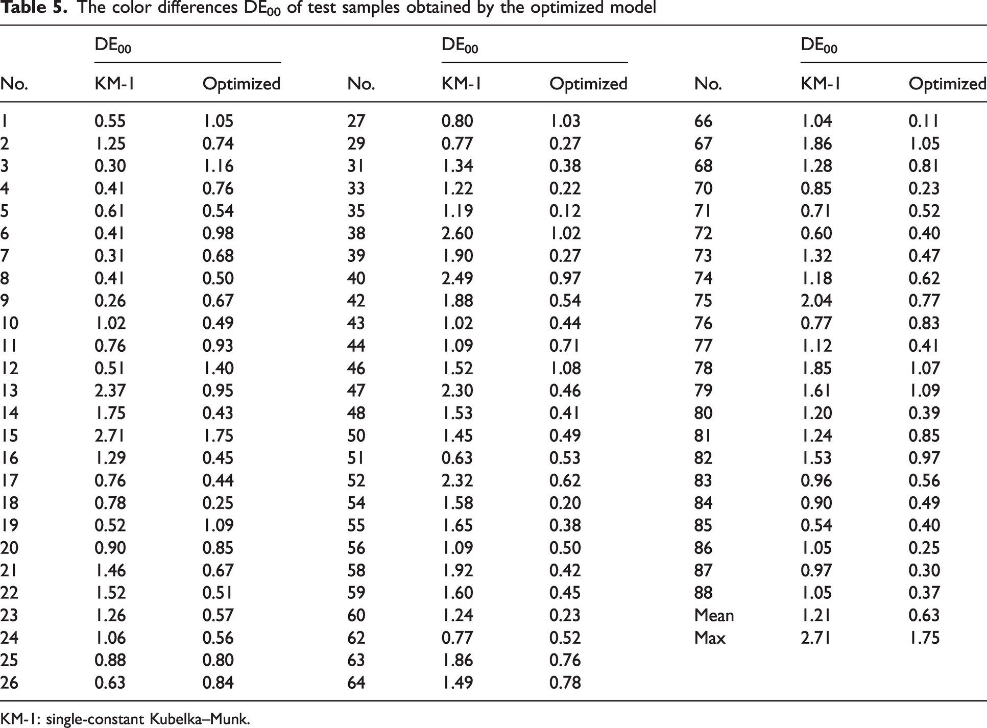
A total of 74 test samples in two-, three-, four- and five-blends were employed to test the validity of the proposed model. Firstly, we substituted the coefficients of Table 4 into Equation (9) to modify the (K/S) mix,λ of two-, three-, four- and five-blends based on the KM-1 model. Secondly, the color differences DE00 of all testing samples were computed based on the CIE2000 formula successively, as shown in Table 5.
The color differences DE00 of test samples obtained by the optimized model
KM-1: single-constant Kubelka–Munk.
The results shown in Table 5 led to the conclusion that the average and maximum color difference DE00 of all test samples on the modified method were improved to 0.63, 1.75 from 1.21, 2.71 of the KM-1 law in succession. Only some samples with a slightly larger DE00 based on the proposed method exist, which are acceptable and possibly caused by the spectral correction. In addition, the original reflectance measured by the Datacolor 600 spectrophotometer and predicted reflectance of 74 test samples and 14 training samples were converted to their corresponding L*a*b* color values. After that, the actual colors of all fiber blends were compared with the predicted ones via this method in pictures, as presented in Figure 5. In this picture, the marked parts with sample numbers of colored squares are the actual colors and the remaining parts are the predicted ones. Real images of the samples taken by the camera can be seen in Figure 2.
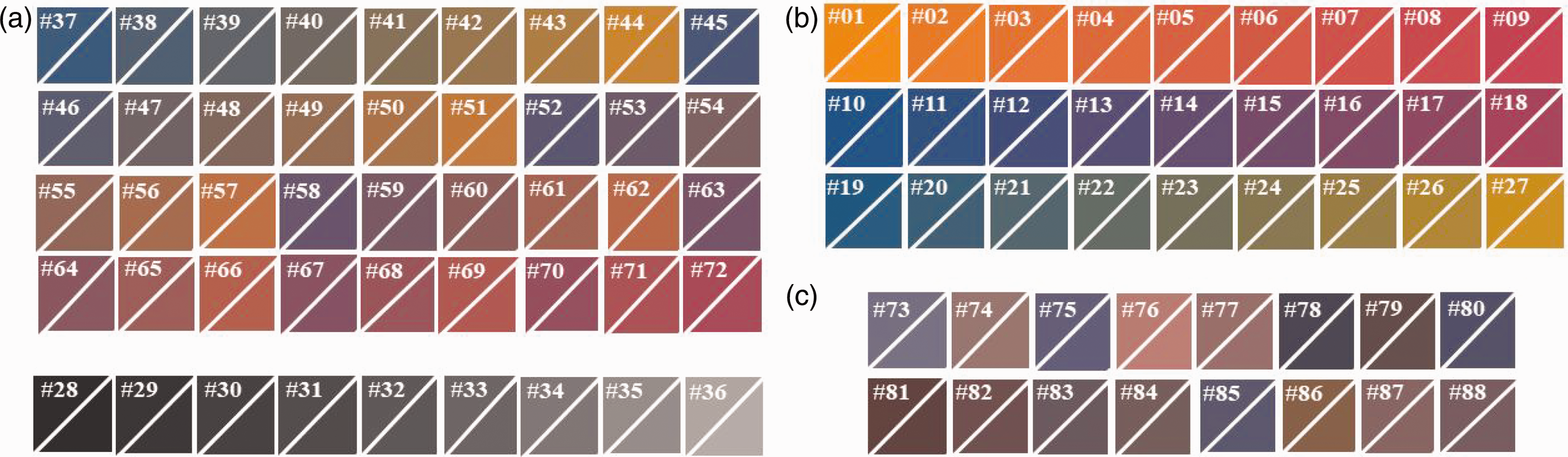
Color comparison of all samples between the measured (number marked) and predicted colors based on this method: (a) RYB fiber blends and WK fiber blends; (b) two-component fiber blends (RY, RB, YB) and (c) four- and five-component fiber blends (RYBW, RYBK, RYBWK). R: red; Y: yellow; B: blue; W: white; K: black.
Comparison with other prediction models
Four kinds of common color prediction laws were employed to compare with this optimized model due to its further demands of effectiveness verification, namely the KM-2 model, KM-1 model, S-N model and Friele model. In particular, their numbers of training and testing samples were set to be the same as those of this proposed model for comparison, except the KM-1 law with no training samples. Meanwhile, the empirical coefficients of the S-N and Friele models were 0.09 and 0.28, respectively, increasing from 0 to 1 at intervals of 0.01 to achieve the least mean color difference. Finally, the predicted color differences of each model were represented by a box diagram, and their statistic results are shown in Figure 6.
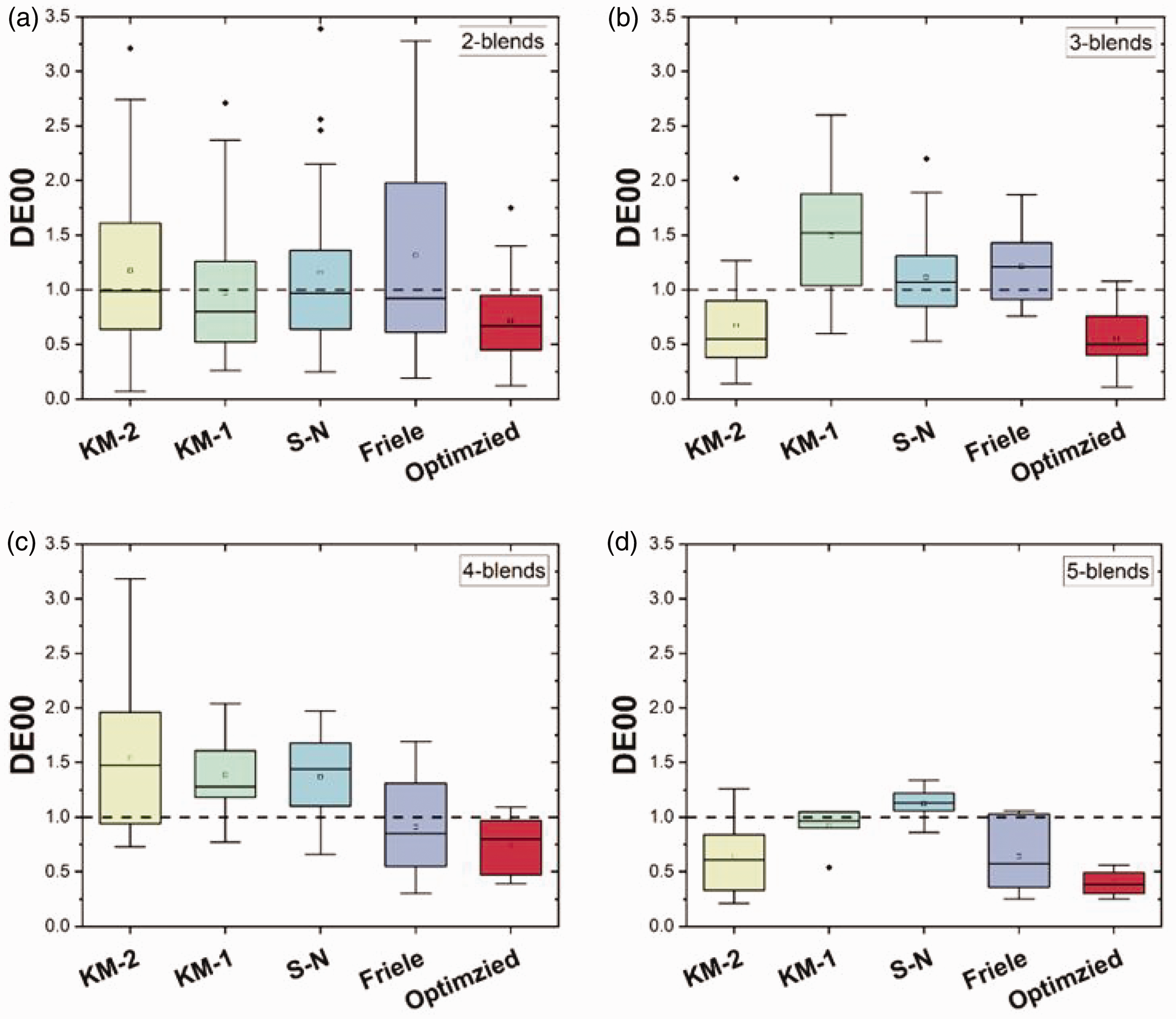
The color difference DE00 compared with other models: (a) comparison of two-blend samples; (b) comparison of three-blend samples; (c) comparison of four-blend samples and (d) comparison of five-blend samples. KM-2: two-constant Kubelka–Munk; KM-1: single-constant Kubelka–Munk; S-N: Stearns–Noechel.
As illustrated in Figure 6, the mean DE00 values obtained by this optimized model were apparently smaller than those of the other models for two-, three-, four- and five-blends. In addition, variations of DE00 on the new method also mostly performed better, except those for three-blends whose difference was not significant compared with the optimal one based on the KM-2 model. This could also be analyzed for each sample in detail in Figure 7. As can be seen, the color difference DE00 of most samples acquired based on this model were below 1, and almost all the remaining ones exceeded 1 and were very close to 1, except for two, which were above 1.25. By contrast, other models had large fluctuations and poor accuracy (Figure 7(a)). Besides, the spectral reflectance of two samples, #12 and #15, had the highest DE00 values of above 1.25 based on this method, and are shown in Figure 7(c). The reflectance curve of sample #12 based on this method was close to the actual and original ones. Obviously, the reflectance of sample #15 based on this optimized model was much closer to the real values than that based on the KM-1 model, although it has a large DE00 of 1.75. At the same time, the mean DE00 of different numbers of primary fibers via this method all became constant at around 0.5, whereas at least half of those samples based on other models had mean color differences greater than 1 (Figure 7(b)). Similarly, as listed in Table 6, the average, maximum and variation of the DE00 color difference gained by the optimized model were all smaller than that obtained by the other models, showing better prediction performance and more stable applicability. Notably, a maximum DE00 based on the optimized model was observed as 1.75 for the No.15 sample in two-blends, and relatively large DE00 values were also computed as 1.67, 2.71, 2.15 and 2.11 for this sample based on the KM-2, KM-1, S-N and Friele models, respectively. Therefore, these large errors were considered to probably come from random errors in the sample preparation. More importantly, the average and maximum values of color difference for the 74 test samples based on the optimized model were only 0.63 and 1.75, as shown in Table 6, which were much lower than those of the KM-2 model (∼1.03 and 3.21), KM-1 model (∼1.16 and 2.71), S-N model (∼1.16 and 3.39) and Friele model (∼1.11 and 3.28).
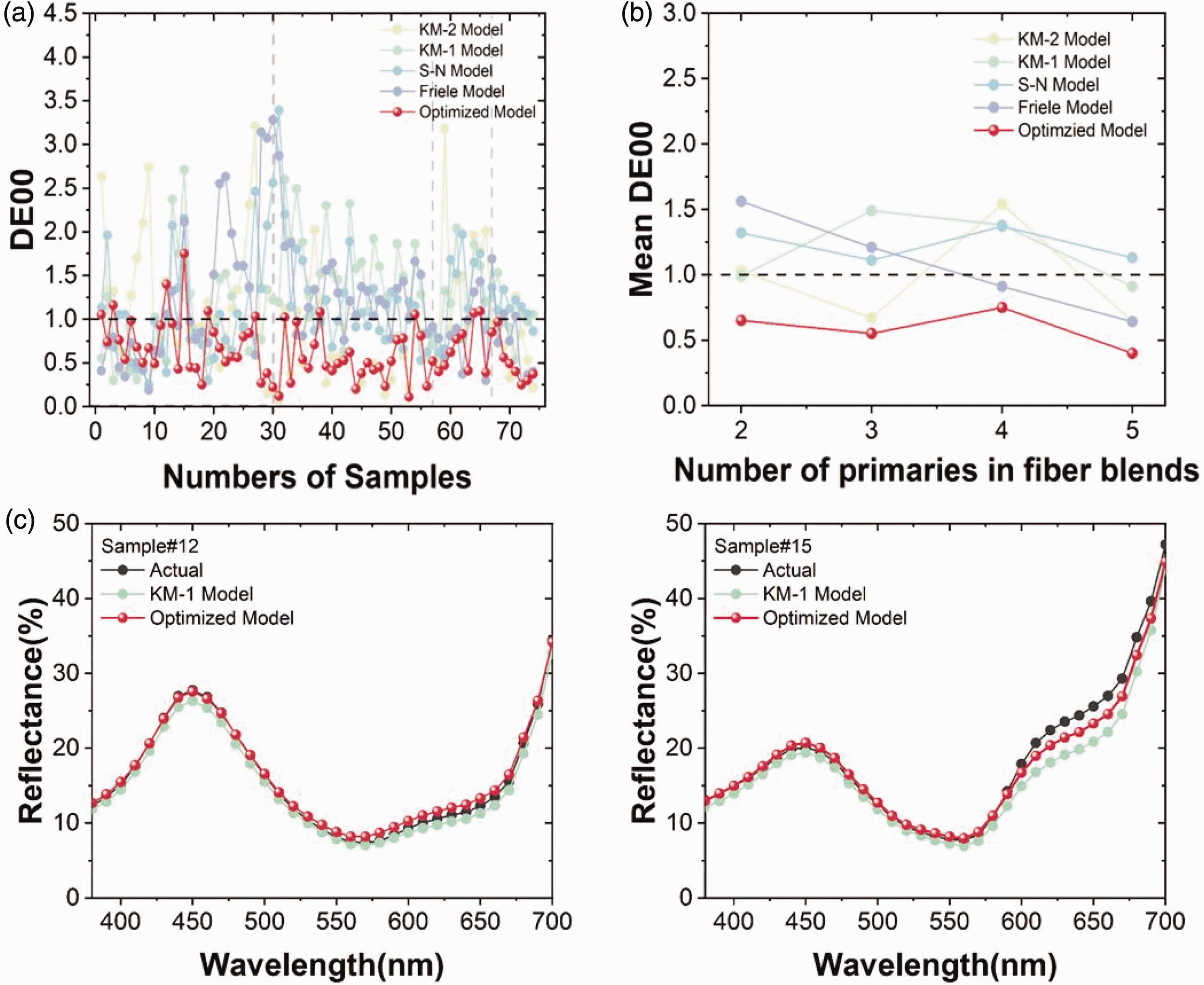
Color matching results of 74 test samples in terms of DE00: (a) color difference DE00; (b) average color difference DE00 for different component blends and (c) comparison of reflectance curves of the #12 and #15 samples obtained by the optimized model and single-constant Kubelka–Munk (KM-1) model. KM-2: two-constant Kubelka–Munk; S-N: Stearns–Noechel.
The color prediction results for the test samples
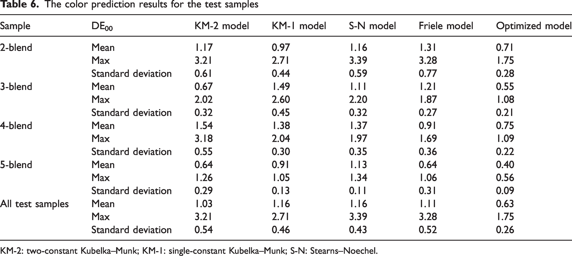
KM-2: two-constant Kubelka–Munk; KM-1: single-constant Kubelka–Munk; S-N: Stearns–Noechel.
Equally important, Figure 8 and Table 7 are shown to evaluate the distribution of DE00 on different models for the 74 test samples. It is revealed that 63 out of 74 test samples (that is, 85.13%) had color difference DE00 of less than 1 on the optimized model, which was higher than those on the other models. Surprisingly, as the range of color difference DE00 expanded to 0–1.1, the percentage of specimens involved based on the optimized model increased dramatically to 95.94%, which was significantly greater than that using the KM-2 (63.51%), KM-1 (45.95%), S-N (51.36%) and Friele (54.05%) models. In particular, other four methods had about six or seven samples with color difference DE00 above 2, while the DE00 color difference values of the optimized model were all smaller than 2.
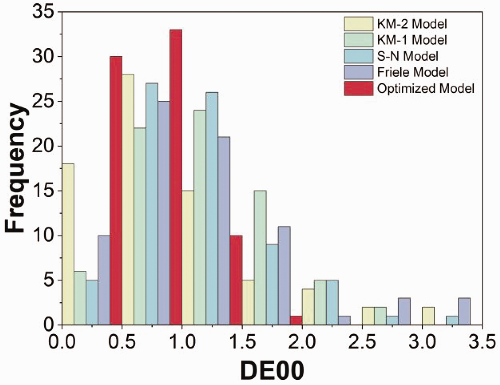
The frequency of color difference DE00 of different models. KM-2: two-constant Kubelka–Munk; KM-1: single-constant Kubelka–Munk; S-N: Stearns–Noechel.
Color difference distribution for test samples
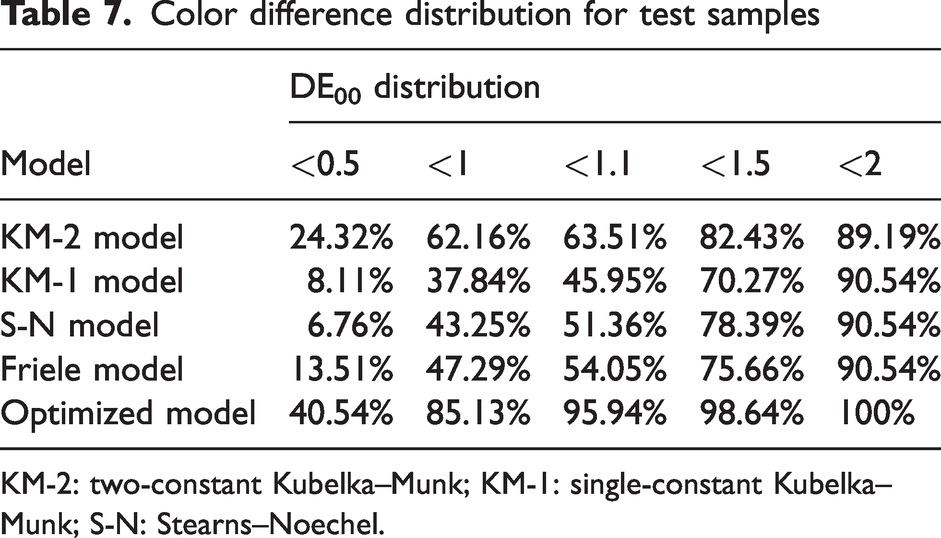
KM-2: two-constant Kubelka–Munk; KM-1: single-constant Kubelka–Munk; S-N: Stearns–Noechel.
What is more, so as to further ensure the validity of the optimized model, it was also compared with recent research on pre-colored fiber blends using the modified KM method. Zhang et al. 25 tested 34 blending fibers based on the modified KM-2 law. For the distribution of color prediction results in his study, as the range of color difference DE00 expanded to 0–1.5, the percentage of the 34 samples increased to merely 79.41%, which was lower than that of our model (98.64%). Thus, it could be appreciated that this spectra optimized method based on the KM-1 model can predict the color of fiber blends accurately by solving problems of the interaction among different component fibers.
Conclusions
This paper proposed an optimized combined spectral calibration model based on the KM-1 law for color prediction of pre-colored fiber blends. In particular, the spectral correction combined equation innovatively consisted of colored and non-colored fiber parts, and was constructed with (K/S) act,λ and (K/S) mix,λ of training samples at different wavelengths. This spectral correction method requires only 14 training samples in color prediction for fiber blending samples composed of the primary fibers. It solves the inapplicable problem of Duncan’s additivity theory for color prediction in pre-colored fiber blends and provides significant assistance to understanding the possible interaction mechanism in pre-colored fiber blends from a new perspective.
The above method was experimentally confirmed that the prediction results of the optimized model for pre-colored fiber blends are highly consistent with the actual ones. Also, its accuracy was demonstrated to be much better than other models using a total of 74 test samples, exhibiting a much lower mean color difference (0.63) than that of the KM-2 model (∼1.03), KM-1 model (∼1.16), S-N model (∼1.16) and Friele model (∼1.11). Besides, the color difference distribution of the optimized model was obviously superior to that of the other models, indicating a much higher percentage (85.13%) of samples with a DE00 below 1. In particular, as the range of DE00 expanded to 0–1.1, the percentages of specimens based on the optimized model was sharply enhanced to 95.94%, and the DE00 values of all samples based on this optimized model were all smaller than 2. In conclusion, the optimized model was verified to be appropriate and effective and could be applied to color prediction of pre-colored fiber blends with an ideal average color difference DE00 (0.63) and excellent color difference distribution using a small number of training samples. Different kinds of fiber blending samples, such as polymer and wool fibers, will be prepared to extend the applicability of the proposed model in future work, and the mechanism of mixing pre-colored fiber will be lucubrated unceasingly to further improve the precision of this model.
Footnotes
Declaration of conflicting interests
The author(s) declared no potential conflicts of interest with respect to the research, authorship, and/or publication of this article.
Funding
The author(s) disclosed receipt of the following financial support for the research, authorship, and/or publication of this article: This work was supported by the National Natural Science Foundation of China (52003244), the Science Foundation of Zhejiang Sci-Tech University (ZSTU) (20202092-Y) and the Outstanding Doctors Foundation of Zhejiang Sci-Tech University (2020YBZX15).
