
Abstract
Fiscal packages usually capitalise into house prices. Yet if enough land for construction is available, housing developers could supply new houses and capitalisation may disappear. This paper provides a theoretical model in which income taxes and public services capitalise at lower rates when housing supply elasticity increases. Using an empirical linear interaction model, we estimate the impact of available land for construction on capitalisation rates with a panel of Swiss communities. Results indicate that fiscal variables do not capitalise differently in communities where housing supply is constrained by land availability. Thus, land availability is a necessary but not sufficient condition for capitalisation to disappear.
1. Introduction
Households usually bid higher prices for houses in communities with lower taxes and higher public service levels to obtain their preferred fiscal package. This leads to capitalisation of fiscal differences into house prices. In his seminal paper, Oates (1969) confirms empirically that taxes and public expenditures are capitalised into property prices. Many papers confirm Oates’ result in the subsequent empirical capitalisation literature: Oates (1973), Johnson and Lea (1982), Reinhard (1981), Richardson and Thalheimer (1981), Yinger et al. (1988), Palmon and Smith (1998) and others report significant and negative tax capitalisation.
However, authors such as Edel and Sclar (1974), Henderson (1985) and Henderson and Thisse (2001) state that capitalisation should not occur in equilibrium if land and housing developers react to fiscal differences between communities. Housing developers supply new houses in fiscally attractive communities until prices are equalised. As a result, fiscal variables do not capitalise. There is some empirical evidence supporting the no capitalisation hypothesis: Wales and Wiens (1974) and Gronberg (1979) do not find capitalisation of taxes into property values, while Edel and Sclar (1974) show that the degree of capitalisation decreases over time. Thus, there is an old conflict in the theoretical and empirical literature as to whether capitalisation of fiscal variables really occurs or not.
This paper contributes to the debate by comparing differences in capitalisation of fiscal variables between communities with available land resources for construction and communities where land for construction is scarce. In a stylised theoretical model which combines the basic ideas of the two competing literature branches, we show that capitalisation of fiscal variables depends on the elasticity of housing supply. If housing supply is perfectly elastic due to ample construction possibilities, the reasoning of Edel and Sclar (1974) as well as of Henderson (1980, 1985) can be applied. In equilibrium, fiscal variables do not capitalise into property values. On the other hand, if housing supply is inelastic because of land scarcity, capitalisation persists as price differences are then driven by the demand side and suppliers cannot compensate demand shocks. Communities with small construction areas should see higher capitalisation. If no construction areas are available, supply cannot react even if enterprises would like to build new houses. Supply may only react if land for construction is available. If available land induces supply reactions, then capitalisation rates should be lower in communities with ample construction opportunities. Therefore, the availability of land for construction is a necessary condition for housing supply reactions.
We analyse empirically whether there is higher capitalisation of fiscal variables when construction areas are scarce. We use a panel dataset of 169 local jurisdictions from 1998 to 2004 in the Swiss Canton of Zurich which includes a comprehensive list of controls for public spending, mobility issues concerning individuals and location-specific characteristics. Our dataset allows us to study capitalisation effects of different public expenditure categories as opposed to most of the literature. Additionally, we analyse for the first time the influence of the availability of land for construction on capitalisation in a European case, which differs from cases in the US in terms of regulatory regimes for construction. Two approaches allow us to identify differences in capitalisation rates over communities depending on construction space availability. The first approach is to divide the dataset into two samples, a ‘no space available’ and a ‘space available’ set. Capitalisation coefficients of fiscal variables should be smaller for the ‘space available’ set if housing suppliers react to differences in capitalisation. In a second step, we use directly the amount of available land for construction and interact it with all fiscal variables. If available land for construction is not sufficient to induce supply reactions, we should observe insignificant interaction effects.
The general finding of this paper is that capitalisation does not significantly diminish when more land for construction is available. Even though capitalisation of fiscal variables is usually lower for communities in the ‘space available’ set, differences are not statistically significant. Thus, empirical evidence seems to support the pro-capitalisation faction. Available land for construction is only a necessary, but not a sufficient, condition for supply to react. Instrumental variable estimates with geographical instruments show that the results are not driven by politically induced changes in the amount of available construction area within different communities.
The results indicate that housing supply reactions do not only depend on the relative scarcity of land. Thereby, we complement the existing literature on capitalisation and land availability which pertains to the US. Instead of using land availability directly, Brasington (2002) argues that public goods packages should capitalise at a higher rate near the urban centre due to high population density and land scarcity, while capitalisation should be lower at the urban edge. Using data from the Ohio, he does not find any robust results for taxes but his hypotheses are confirmed for other aspects of public good provision. Hilber and Mayer (2009) show with data from Massachusetts that capitalisation of school spending decreases when a jurisdiction has more developable land.
Our results provide new and additional insights into the existence and persistence of capitalisation of fiscal variables for a European case. Housing supply cannot be elastic if land for construction is scarce. However, it will not necessarily be elastic if land for construction is available. Housing supply reactions are likely to be influenced by other factors than only land for construction. Regulatory regimes, political zoning decisions, uncertainty concerning the stability of fiscal differences between communities and the opposition of existing property owners (see Fischel, 2001) distinguish regions in Europe from regions in the US in general and also regions within the US may distinguish themselves. Existing property owners may try to prevent developers from new construction to maintain their property values and avoid uncertainty. Thus, available land for construction is only a necessary but not a sufficient condition for housing supply reactions to occur and our results indicate that capitalisation of fiscal variables may persist even in communities with ample construction opportunities.
The sequence of this paper is as follows. Taking account of the intensive discussion in the literature, we develop a simple theoretical model in section 2 that shows the link between demand and supply in the housing market with capitalisation of income taxes and public services. Section 3 presents two approaches to identify differences in capitalisation between communities where land is available and communities where land is scarce. The main variables for capitalisation used in the literature as well as additional controls are employed in our setting. Section 4 summarises the results, offers interpretations and concludes.
2. Basic Model
To illustrate the different ideas of the capitalisation debate, we present a simple stylised model with income taxes which puts together the two competing strands of literature.
1
We consider a metropolitan area composed of I jurisdictions and inhabited by N residents who are perfectly mobile and have identical tastes and incomes. A household’s income

with standard properties, taking account of the budget constraint

where,
When looking for a jurisdiction to live in, households consider tax–expenditure combinations as given and the community’s budget constraint does not enter the maximisation problem (see Yinger 1982). The household’s maximisation problem yields the indirect utility function

All N residents of the metropolis must be housed such that
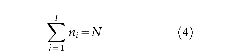
where, ni is the number of households residing in jurisdiction i. Equilibrium requires that housing market clears in each jurisdiction

where, hi(pi) denotes housing demand per resident; and Hi(pi) aggregate housing supply in community i. 2 Substituting (5) in (4), we obtain
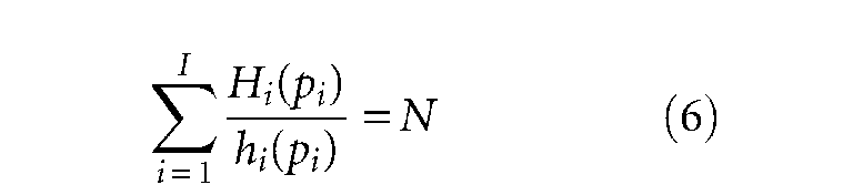
Equations (3) and (6) implicitly define equilibrium house prices as a function of disposable income and thus taxes, public goods as well as price elasticities of housing supply and demand. We differentiate (3) and (6) with respect to gi. After appropriate substitutions and solving for
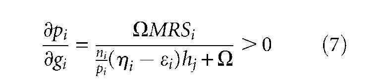
where,
Under standard assumptions regarding housing demand and supply elasticities (
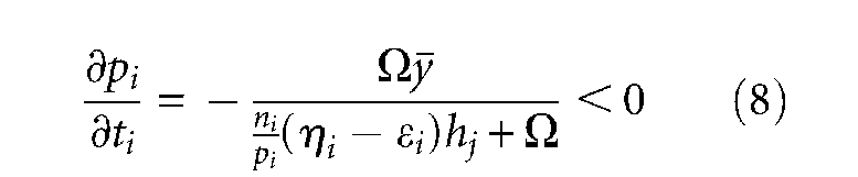
An increase in tax rate capitalises negatively. As already argued by Yinger (1981, 1982) for inelastic housing supply, public goods capitalise positively whereas taxes capitalise negatively. However, if enough land for construction is available, supply may be perfectly elastic and (7) and (8) indicate for
The supply elasticity in a community may increase when more land is available. We can compute the effect of an increase in housing supply elasticity on capitalisation by differentiating (7) and (8) with respect to

Thus, the model predicts that, if available land induces supply reactions, the higher supply elasticity negatively affects the extent of capitalisation of public goods and taxes. We test empirically whether land availability leads to differences in capitalisation of fiscal variables.
3. Estimation of Differences in Capitalisation
3.1 Data
For our purposes, we use a panel dataset of 169 communities from 1998 to 2004 for the Swiss Canton of Zurich which includes a comprehensive list of controls for public expenditures, mobility issues concerning individuals as well as location-specific characteristics. The variables, their definition, sources, medians, means and standard deviations are given in Table A1 in the Appendix. The metropolitan area of Zurich has approximately 1.3 million inhabitants which makes it the most populous of all 26 Swiss cantons. Moreover, it is also one of the most densely populated areas in Europe. The City of Zurich is the economic core of the agglomeration and the biggest city in Switzerland. Including commuters, around a million people either work or live there. 3 Because of their high degree of autonomy, the communities of the canton of Zurich are an ideal laboratory in order to test the influence of differences in capitalisation rates of local government expenditures and taxes.
As the dependent variable, we use the price of a standardised single-family house with five rooms, two bathrooms, 450 square metres garden area, 750 cubic metres volume, end-terrace house and one garage space. Such a price is available for every community over the years 1998 to 2004. The data were obtained from the Cantonal Bank of Zurich, the largest real estate bank in the canton, which evaluates houses by the sales comparison approach based on actual transactions. The sales comparison approach is a commonly used valuation method in real estate appraisals. The Cantonal Bank of Zurich uses a set of over 15 000 house sales in the canton to determine the magnitude of construction-specific attributes—such as the number of rooms, the age of the house and the number of bathrooms—on property values in the canton’s communities.
Our independent variables were obtained from the Statistical Office of the Canton of Zurich, the Secretary for Education of the Canton of Zurich, the Financial Statistics of the Canton of Zurich and the Cantonal Bank of Zurich.
We use a number of fiscal variables including taxes and different expenditure categories that allow us to analyse fiscal bundles as proposed by our model. Our dependent variable and all fiscal variables are tested for stationarity for each community using the KPSS test. All tested variables are either stationary or trend stationary. 4 The canton’s local jurisdictions are autonomous: Swiss communities have the possibility to levy income taxes via a municipal tax rate (collection rate) fixed by the community itself on a yearly basis. The collection rate is added to the cantonal base tax (in German: allgemeine Staatssteuer) which varies from canton to canton (see Stull and Stull, 1991, for income tax capitalisation in the US). Following the introduction of a harmonised public accounting system for bookkeeping and budgeting, reliable and consistent municipal financial data for different expenditure categories are available for all communities in our dataset. The literature often focuses on education aspects and school characteristics when analysing house prices (see, for example, Brasington, 1999; and Figlio and Lucas, 2004). We include a measure of the distance to the next school in metres and control whether the school is managed by the community itself or a separate school community (see Frey and Eichenberger, 2002). Furthermore, we take account of the class size in primary schools. 5
In the empirical analysis, it is common to control for median incomes, population density and the fraction of elderly people in the community. Also, we take account of mobility issues by including the fraction of commuters that leave the community every day. The unemployment rate and the fraction of foreigners are also used for robustness tests and represent additional controls for population and demographic effects. Finally, our dataset allows us to control for location-specific variables. These include a view of the lake, south and west situation in the community, the distance to Zurich main station and therefore to the economic core, distance to the next shopping centre and the pollution level. 6
In our analysis, we do not include the cities of Zurich and Winterthur. As opposed to the other communities, they are considered as cities and have a different structure: Zurich and Winterthur have each a number of separate districts that form these cities. The districts differ in important aspects such as median incomes, unemployment rates and the fraction of foreigners. Furthermore, Zurich is the centre of the canton and we control for the distance to the centre in order to treat mobility issues. Most importantly, the two cities are large with respect to the rest of the communities in the canton. 7
To test our main prediction, we use available construction area as a proxy for housing supply elasticity. Available construction areas as reported by the Office for Spatial Planning and Surveying denote land areas in square metres already zoned for residential use but not yet developed. A developer may start building residential real estate if his/her building project has been approved. Available construction areas do not include land zoned for other purposes such as farming or industry which might be potentially rezoned as rezoning processes usually require a time-horizon of many years and involve uncertainties. According to estimates by the Office for Spatial Planning and Surveying, undeveloped construction areas—i.e. the available construction area—in the Canton of Zurich could accommodate approximately 155 000 additional inhabitants, over 10 per cent of the current population. Figure 1 plots a histogram of average available land for construction for the years analysed.
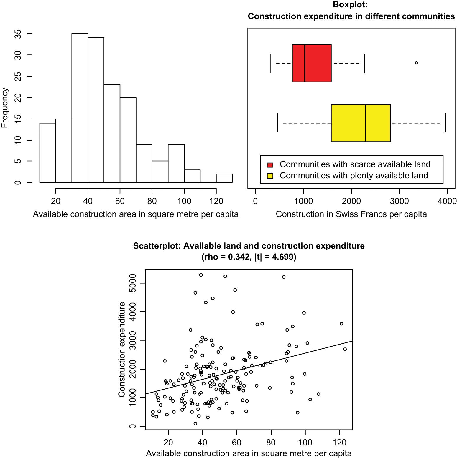
Available construction area per capita and building activity.
The available construction area for individual communities ranges from below 20 square metres per capita to over 130 square metres per capita, enabling us to analyse the effects of construction possibilities on capitalisation rates. The boxplot presented in Figure 1 shows that construction expenditures per capita for family houses in the sample of communities with a low number of square metres of available construction area per capita (upper boxplot) are usually lower than construction expenditure per capita for family houses in communities with a high number of square metres of available construction area per capita (lower boxplot). Even the first quartile of construction expenditure per capita in communities with plenty of available land is higher than the median of construction expenditure per capita in communities with scarce available land without holding constant other intervening variables such as school, demographic, socioeconomic and location-specific characteristics of communities. Thus, more construction seems to take place in communities where more land for construction is available. A similar relationship can be seen in the scatterplot for available land for construction and construction expenditure per capita.
3.2 Analysis of Separate Samples
Our theoretical model shows that the extent of capitalisation declines when the elasticity of housing supply increases. We identify whether land availability is sufficient for supply reactions to happen and for capitalisation of fiscal variables to vanish by using two different methods which allow us to identify differences in capitalisation of fiscal variables over space. Each of the approaches uses an amenity model setting which is common in the literature (see, for example, Brasington, 2000, 2002).
The first approach is to divide the dataset into two distinct samples. The average available construction area in the year 1998 over all 169 communities in the dataset was 55.425 square metres per capita. Communities with less than 55.425 square metres of available construction area per capita form the ‘no space available’ set while communities with more than (or equal to) 55.425 square metres per capita form the ‘space available’ set. A dummy variable denoted
Testing for decreasing capitalisation over space when land is available (dummy)

Notes: The impact of a 1 per cent increase of the mean of the respective independent variable on property prices. The left-hand-side variable in all regressions is the average price of a comparable single-family house for the respective years 1998 to 2004 across 169 municipalities. Robust standard errors in parenthesis. a indicates a significance level of below 1 per cent; b indicates a significance level between 1 and 5 per cent; c indicates significance level between 5 and 10 per cent.
Taking a look at the coefficient estimates of specifications (1) and (2), we find—like Oates (1969), Stull and Stull (1991) and other authors—that the tax rate has a negative and significant influence on house prices. 9 Similarly, aggregate public expenditures increase house prices significantly. While class size has a significant negative impact on house prices for both samples, the distance to the next school has a negative and significant effect only in the ‘space available’ sample. The form of school organisation in separate school communities does not have any significant impact. House prices react positively and significantly to higher median incomes as commonly documented in the literature. More densely populated areas with a higher fraction of elderly people have higher prices too, but the significance depends on the sample chosen. Commuting imposes costs on individuals and capitalises negatively and significantly in the ‘space available’ sample. Unemployment rate negatively affects house prices in the ‘no space available’ sample. The fraction of foreigners has a positive and significant influence on house prices in both specifications because of a large number of well-educated expatriates in the Canton of Zurich. All location-specific controls have the expected signs: the average view of the lake and good situation increase prices, distance to the centre and the next shopping facility as well as the level of air pollution decrease them.
Oates’ (1969) estimations were criticised by Henderson and Thisse (2001) and by a number of other authors who argued that capitalisation rates should tend to zero because of housing supply reactions. As more land for construction is available, housing supply can react more easily to differences in fiscal packages. Consequently, capitalisation of fiscal variables is expected to be lower in communities with ample construction possibilities. Looking at the results for specifications (1) and (2), we find that a 1 per cent increase in the mean income tax rate reduces house values by 1298.80 Swiss francs in the ‘no space available’ set and by 745.40 Swiss francs in the ‘space available’ set. Thus, tax capitalisation is lower in communities where housing supply can react due to more available land. Similarly, a 1 per cent increase in aggregate expenditures raises house values by 669.80 Swiss francs when fewer construction areas are available and by 560.00 Swiss francs when more construction areas are available.
Specifications (3) and (4) use diverse public expenditure categories instead of aggregate public expenditures. Again, we find that taxes capitalise less in jurisdictions with more construction space. Similarly, a 1 per cent increase in public expenditures for culture raises house values by 222.70 Swiss francs when land for construction is scarce, as opposed to 162.40 Swiss francs when construction possibilities are available. For social expenditures, the effects are less robust as capitalisation of this category is lower in the ‘no space available’ set. Capitalisation for administrative expenditures is negative and not significant in both samples. Finally, health expenditures have again a marginally larger impact when construction space is scarce.
Even though estimates for separate samples indicate that capitalisation is lower in communities with more construction areas per capita, it is unclear whether these differences are statistically significant. Point estimates of tax coefficients in columns (1)–(4) are significantly different from zero, but not necessarily significantly different from each other. For public expenditures, point estimates are relatively close. To test formally for such significant differences in capitalisation across communities, the dummy variable for land availability is interacted with tax rates, aggregate public expenditures as well as different public expenditure categories. Housing supply can be sufficiently elastic only if construction space is available. Moreover, if housing development reacts to capitalisation, we expect tax interaction coefficients to be positive and expenditure interaction coefficients to be negative—i.e. capitalisation in communities with supply reactions should be lower. In columns (5) and (6), we estimate a dummy interaction model to test whether the differences in capitalisation in the sets are statistically significant. The identifier for whether construction areas are scarce or easily available,
To make sure that these results are not only valid for the chosen threshold of the identifier
3.3 Linear Interaction Model
Our second method to evaluate differences in capitalisation of fiscal variables is to analyse a linear interaction model. The empirical model interacts a standardised measure for available construction area with taxes and expenditure variables. 11 If available land for construction is sufficient to induce supply reactions to fiscal packages, then the interaction of taxes with available construction areas should be positive while the interaction of public expenditures with available construction areas should be negative—i.e. capitalisation tends to decrease with more construction space within the communities. Table 2 reports the results.
Testing for decreasing capitalisation over space when land is available (interaction + IV)

Notes: The impact of a 1 per cent increase of the mean of the respective independent variable on property prices. The left-hand-side variable in all regressions is the average price of a comparable single-family house for the respective years 1998 to 2004 across 169 municipalities. Robust standard errors in parenthesis. a indicates a significance level of below 1 per cent; b indicates a significance level between 1 and 5 per cent; c indicates significance level between 5 and 10 per cent.
The base effects in column (1) have the expected signs and are significant. Their impacts expressed in Swiss francs on house prices are comparable with previous estimates. The interaction effect for taxes and the standardised measure for available construction area have a positive sign but are insignificant. The interaction effect for aggregate expenditures is negative and insignificant. Thus, capitalisation of fiscal variables is not significantly different when more space for construction is available.
In specification (2), we estimate the interaction model with disaggregate expenditures. Expenditures for culture, social welfare and health have a positive and significant impact on house prices, while administrative expenditures capitalise negatively but insignificantly. All interaction effects are insignificant and consequently no housing supply reactions can be found even though more space for construction was available.
So far, we have only reported results from OLS estimations. However, such estimates could suffer from possible simultaneity bias. 12 Available construction areas do not only depend on geography but also on political decisions by citizens, and thus on their property values. Even though available construction space in the Canton of Zurich changed slightly over time, it is not necessarily exogenously given but might be the result of fiscal preferences. It could be possible that high house prices induce communities either to restrict the amount of land for construction to preserve house values or induce them to increase the amount of land for construction to make additional profits by selling land. In either case, additional land for construction could emerge endogenously. This, of course, would leave our coefficient estimates for available land and the interaction effects biased. To address this problem, we estimate 2SLS regressions in columns (3) and (4). We use, as instruments, geographical variables which are independent of local political decisions. The first instrument indicates whether the community is next to the cities of Zurich or Winterthur and consequently forms part of the densely populated centre. As a second instrument, we look at if the community lies near the cantonal border where densities are lower and more farming land might be rezoned and used for construction. Finally, we take the fraction of traffic area as a measure of communal development as well as communal importance. This measure is stable over time and usually only influenced by cantonal instead of local decisions. All instruments do not have a directly discernible influence on house prices and on fiscal variables when controlling for measures of density and distance to the centre. Concerning the quality of the instruments, F-tests for the first-stage variable are highly significant for explaining available land. 13 The J-statistics which deal with the over-identifying restrictions confirm the quality of the instruments. The coefficients of the fiscal variables and the interaction effects are similar to the OLS estimates. Taxes capitalise negatively and significantly while aggregate expenditures as well as the different expenditure categories capitalise positively and significantly. 14 The hypothesis that housing supply reacts more when construction space is available can be rejected as none of the interaction effects is statistically significant.
Finally, to ensure that these results do not only depend on a specific time-frame chosen, we investigate the relationships for each year individually. The respective specifications (1) and (2) of Table 2 are estimated separately for the years 1998 to 2004 in Table A3 in the Appendix. The base effects for taxes remain negative and significant. Public expenditures usually have a positive and significant influence. None of the interaction terms with available land for construction and fiscal variables ever turns significant. Thus, housing supply does not influence capitalisation of fiscal variables when more construction area is available.
4. Conclusion
Capitalisation occurs when households bid higher prices for houses in communities with lower taxes and better public services. Part of the theoretical literature argues that fiscal variables capitalise owing to the scarcity of construction space in metropolitan areas. Many empirical papers show that fiscal variables capitalise into house prices. However, some authors argue that capitalisation is only a demand-side phenomenon. If house developers react to differences in fiscal packages, they will provide houses in fiscally attractive communities. Due to potential supply reactions, capitalisation may not occur in equilibrium. According to both views, the question of whether capitalisation exists in equilibrium is a central issue of the theory of local public finance (see Yinger et al., 1988).
We have brought the arguments of the two sides together and have shown how capitalisation depends on the elasticity of housing supply. Assuming an inelastic and upward-sloping supply function, capitalisation of taxes and public expenditures occurs. When housing supply is perfectly elastic, capitalisation does not persist. Using a set of 169 communities from 1998 to 2004 in the Swiss Canton of Zurich, we bring our theoretical insights to the data.
We find support for the pro-capitalisation faction at common statistical significance levels. If housing supply reacts to fiscal differences, supply reactions should be stronger in communities with a higher amount of available construction space. A linear interaction model shows that tax capitalisation is not significantly lower when more land for construction is available. Similarly, public services do not capitalise significantly less in communities with more construction possibilities. Estimates for interaction terms between fiscal variables and available land point to somewhat smaller capitalisation. However, a high variance does not allow us to draw supportive conclusions for the no-capitalisation faction. Housing supply does not react significantly more in communities with more developable land and capitalisation of fiscal variables is not significantly lower in such communities. The yes-capitalisation faction has a point, as house developers do not seem to react to a large extent to fiscal differences over space even if land is available. Capitalisation of fiscal packages persists even if new housing construction is possible. Available land for construction is only a necessary but not a sufficient condition for supply reactions to occur. The elasticity of supply is likely to be influenced by other factors too, such as zoning decisions, uncertainty concerning changes in fiscal variables and existing homeowners’ opposition.
Our results are complementary to those of Brasington (2002) and Hilber and Mayer (2009) who find that capitalisation decreases when space is more readily available in a community. While their studies are based on data for the US, we focus on a European metropolitan area. Available land for construction alone is a theoretically necessary but not a sufficient condition. In the European case, different landscape topography, zoning regulations, fiscal uncertainty and other factors may prevent housing suppliers from reacting despite the availability of land for construction. This view is consistent with ideas by Fischel (2001) that homeowners are reluctant to see new construction and exert political pressure to prevent new development even if land for construction is available. More research is needed to identify the driving-forces behind housing suppliers’ reactions.
Footnotes
Notes
Funding Statement
This research received no specific grant from any funding agency in the public, commercial or not-for-profit sectors.
Appendix
Yearly estimates for testing for decreasing capitalisation over space
| Variable | 1998 ExpAgg | 1999 ExpAgg | 2000 ExpAgg | 2001 ExpAgg | 2002 ExpAgg | 2003 ExpAgg | 2004 ExpAgg | 1998 Categories | 1999 Categories | 2000 Categories | 2001 Categories | 2002 Categories | 2003 Categories | 2004 Categories |
|---|---|---|---|---|---|---|---|---|---|---|---|---|---|---|
| Intercept | 684 000 a (130 200) | 751 358 a (131 800) | 759 100 a (147 600) | 708 103 a (134 400) | 769 900 a (143 700) | 719 000 a (143 300) | 824 900 a (144 700) | 748 900 a (143 000) | 750 087 a (137 400) | 770 892 a (156 300) | 734 400 a (139 800) | 833 600 a (151 600) | 817 400 a (147 900) | 901 400 a (141 300) |
| TaxRate | −984.50 b (460.600) | −1 268.95 a (440.600) | −916.60 c (492.100) | −831.78 c (440.900) | −937.30 c (521.900) | −954.40 c (504.500) | −1 137.10 b (527) | −989.60 b (488.600) | −1 167.27 a (432.400) | −885.71 c (525.200) | −834.12 c (467.100) | −949.50 c (500.600) | −927.95 c (473.600) | −1 175.02 b (466.700) |
| Int(Tax * LandAvailable) | 10.330 (12.420) | 5.131 (13.600) | 14.080 (13.280) | 11.795 (13.390) | 7.907 (16) | 2.970 (14.340) | 1.926 (15.600) | 22.350 (88.840) | 101.492 (78.700) | 150.636 (92.920) | 160 (99.210) | 44.310 (121.600) | 72.470 (124.300) | −96.250 (125.700) |
| ExpAgg | 84.810 a (31.040) | 92.487 a (31.830) | 72.220 b (35.850) | 167.721 a (33.220) | 164.300 a (29.270) | 167.400 a (34.340) | 132.800 a (35.090) | |||||||
| Int(ExpAgg * LandAvailable) | −0.071 (0.773) | −1.016 (0.862) | −0.573 (0.967) | −1.301 (0.969) | −0.264 (0.911) | −0.274 (0.915) | −0.124 (0.822) | |||||||
| ExpCulture | 150.100 c (81.580) | 155.088 c (83.800) | 168.179 c (87.550) | 186.800 b (86.560) | 140.600 c (83.820) | 163.300 c (86.090) | 110.300 (76.950) | |||||||
| Int(ExpCulture * LandAvailable) | −2.062 (2.471) | −3.218 (2.759) | −3.475 (2.604) | −1.242 (2.706) | −0.726 (2.257) | −2.953 (2.470) | −2.312 (2.335) | |||||||
| ExpSocial | 63.160 c (37.290) | 74.833 c (40.350) | 49.532 c (31.780) | 111.400 b (45.750) | 104 b (45.790) | 88.920 b (44.670) | 71.600 c (38.320) | |||||||
| Int(ExpSocial * LandAvailable) | −0.392 (1.449) | 1.585 (1.396) | 0.783 (1.779) | 1.188 (1.710) | 0.113 (1.436) | 0.372 (1.200) | 0.373 (0.949) | |||||||
| ExpAdmin | −62.370 (39.290) | −5.330 (34.410) | −20.866 (35.510) | −8.992 (36.570) | −4.038 (32.550) | −16.120 (28.250) | −9.178 (28.820) | |||||||
| Int(ExpAdmin * LandAvailable) | −1.344 (1.037) | −1.931 (1.374) | −1.137 (1.136) | −0.620 (1.124) | −1.086 (0.853) | −1.194 (0.801) | −2.495 (2.921) | |||||||
| ExpHealth | 137.500 c (70.300) | 97.786 c (60.100) | 88.379 c (54.840) | 249.400 a (52.950) | 308.300 a (73.580) | 343.300 a (91.090) | 337.500 a (113.600) | |||||||
| Int(ExpHealth * LandAvailable) | −1.269 (2.712) | −2.844 (3.392) | −1.204 (2.962) | −1.162 (1.375) | −1.508 (2.427) | −2.191 (3.250) | −3.739 (3.271) | |||||||
| LandAvailable (Continous) | −1 532 (1 535) | −1 387.20 (1 699) | −2 170 (1 655) | −2 206.45 (1 804) | −1 244 (2 038) | −754.100 (1 760) | −85.390 (1 834) | 335.600 (581.300) | 309.004 (696.500) | 830.855 (738.900) | 2.374 (799.600) | 131.600 (793.900) | 162.600 (868.100) | 665.500 (911.600) |
| Other controls | YES | YES | YES | YES | YES | YES | YES | YES | YES | YES | YES | YES | YES | YES |
| Adjusted R2 | 0.879 | 0.875 | 0.871 | 0.890 | 0.898 | 0.892 | 0.887 | 0.879 | 0.877 | 0.871 | 0.890 | 0.898 | 0.895 | 0.894 |
| N | 169 | 169 | 169 | 169 | 169 | 169 | 169 | 169 | 169 | 169 | 169 | 169 | 169 | 169 |

Notes: The left-hand-side variable in all regressions is the average price of a single-family house for the respective years 1998 to 2004 across 169 municipalities. Robust standard errors in parenthesis. a indicates a significance level of below 1 per cent. b indicates a significance level between 1 and 5 per cent. c indicates significance level between 5 and 10 per cent.