Assessing the Impacts of Smart Growth Policies on Home Developers in a Bi-state Metropolitan Area: Evidence from the Portland Metropolitan Area

Abstract

While there are many empirical studies examining the effectiveness of smart growth policies, few of them study the perspective of developers, the major urban space producers in US cities. This article assesses the impacts of smart growth policies on home developers in the Portland bi-state metropolitan area by developing home developer location choice models. The study shows that home developers in the region are sensitive to most smart growth policies being implemented in the region, but they react to them differently across the border between Oregon and Washington due to their different land use planning systems. The findings suggest that smart growth policies impact single- and multifamily home developers’ location choices differently and that home developers exhibit strong spatial inertia in their location choice.

Introduction

There are extensive empirical studies on the impacts of smart growth policies; however, very few of them consider the perspective of individual decision-makers and, to our knowledge, none has studied developers as location-aware decision-making agents. Thus, much of the current understanding of the effectuality of smart growth policies lacks a micro-level behavioural foundation. Literature review finds some studies using agent-based models to test the impacts of land use on individuals’ residential location choice, but being household-based represents only the demand side of the land development market. The other side of the market, the provision of housing supply as represented by developers, remains understudied.

Using a unique eight-year housing permit and land use dataset provided by Metro, the elected regional government for greater Portland, Oregon (Figure 1), this study fills this research gap partially by studying the impacts of smart growth policies on home developers’ location choice in the Portland metropolitan area, a bi-state metropolitan area straddling the border between Oregon and Washington, including Vancouver. While numerous smart growth policies have been implemented in the Portland region, this study focuses on three important aspects of smart growth—urban growth containment, transport accessibility and utilisation of existing infrastructure—while controlling many other relevant variables. This study considers three research questions

To what extent do smart growth policies influence developers’ location choice in the Portland metropolitan area?

Do smart growth policies have different impacts on developers’ location choice in Oregon compared with across the border in the state of Washington?

Do single-family home (SFH) and multifamily home (MFH) developers exhibit different preferences for their project location choices?

To answer those research questions, we have developed a set of developer location choice models. In this study, we define a SFH as a housing structure with only one detached dwelling unit; a MFH is a housing structure composed of more than one unit. We have modelled SFH developers and MFH developers separately, as distinct market segments. In the remainder of this paper, we will discuss the Portland metropolitan area and its smart growth policies; review some of the prior research that has examined the effectiveness of these policies; discuss the data used for the current study, the model design and estimation results; and conclude with a summary of important findings.

Portland Metropolitan Area and Its Smart Growth Policies

Straddling the border between Oregon and Washington, the Portland metropolitan area is a bi-state metropolitan area composed of four counties: Multnomah, Washington and Clackamas in Oregon, and Clark County in Washington (Figure 1). For transport planning purposes, the four-county region is divided into 1998 traffic analysis zones (TAZs), which we use as spatial units for the location choice models developed in this study. As Figure 1 shows, the sizes of TAZs vary, but 60 per cent are smaller than 1 square kilometre and 80 per cent are smaller than 2 square km.

Figure 1.

Counties, TAZs and the UGB in the Portland Metropolitan Area.

While the four counties in the region comprise the same housing market, the market functions under two different state land use systems. The three counties in Oregon are served by Metro, the only elected regional government in the US. According to its Charter (Metro, 1992), Metro has the power to require changes in local comprehensive plans to make them consistent with its functional plans. Oregon law also requires local comprehensive plans to be compatible with state-wide planning goals (Abbott, 2002). Metro includes Clark County, Washington (Vancouver area) on its 2040 Growth Concept maps (Metro, 1995), but has no regulatory powers there. The planning and zoning in Clark County is regulated by Washington state laws, which include a Growth Management Act (GMA) enacted in 1990 to guide planning for growth and development in Washington. Notably, while designing their growth management system, the Washington legislature deliberately avoided the top–down planning system found in Oregon (Weitz, 1999) and limited the power of the State to alter the content of local plans (Abbott, 1997).

Portland has an international reputation as a model for smart growth. Among many smart growth policies that have been implemented in the Portland region, the urban growth boundary (UGB) garners the most attention. Figure 1 shows the UGB in the metropolitan area in 2005. The basic purpose of the UGB is to prevent urban sprawl by identifying and separating rural land from urban and ‘urbanisable’ land, thereby providing orderly, efficient transitions from rural to urban use (Metro, 1995). In Clark County, Washington, as required by the GMA, urban growth areas (UGAs) were designated and urban growth is encouraged to be inside them. In this study, we treat the boundary of the UGAs in Clark County, Washington, as its UGB.

As a policy tool, the UGB represents a set of planning policies that regulate land use outside and inside it. A comparison of the state-wide planning goals in Oregon and Washington shows that both the states have land use policies regulating the land use outside the UGB by: protecting agricultural and forest lands, environmentally critical areas and open spaces; restricting the establishment and extension of public facilities; and, controlling residential, commercial and industrial land developments on rural land. While the two states share similar goals in restricting land developments outside the UGB, the regulations on land developments outside the UGB in Clark County, Washington, tend to be less restrictive and traditional sub-divisions of moderately priced houses with large size land lots were still available in the study period.

In addition to the land development regulations outside the UGB, both Oregon and Washington have set state planning goals to encourage mixed-use, high-density and transit-oriented development (TOD) within the UGB. The real effects of those planning goals and policies, however, are highly dependent on the planning and land use regulations by local governments, especially their zoning. The data show that there is more land zoned for medium- and high-density residential use and mixed use in the three Oregon counties than in Clark County, Washington, both in total and proportionally. Compared with Clark County, the Oregon side of the metropolitan area also has a more fully developed bus transit system and light rail and streetcar modes not found in Clark County/Vancouver.

Prior Examination of Portland’s Smart Growth Policies

Previous studies examining the impacts of Portland’s smart growth policies have focused on its UGB, questioning whether it has successfully prevented urban sprawl and encouraged certain growth patterns such as higher land use density, more mixed use and TOD.

Nelson and Moore (1993) divided the fore-mentioned three Oregon counties into four parts based on their locations relative to the Portland UGB. Comparing land use density in these four areas from 1985 to 1989, they concluded that development was being directed to the areas within the UGB, but recognised that considerable development continued outside the UGB. Abbott’s (2002) analysis of multiple data sources concluded that Portland’s UGB had successfully contained new development within it, increased land use density and decreased average new lot size. Further, he noted that almost all the new housing outside the UGB was located in Clark County, Washington.

While these studies report that Portland’s UGB is at least partially achieving its goals, other researchers have come to contradictory conclusions. For example, Richardson and Gordon (2001) argued that Portland is actually statistically similar to Los Angeles in terms of suburbanisation, decentralisation and public transit. Jun’s (2004) study confirms Richardson and Gordon’s argument that Portland has not been successful in sprawl control, citing that Portland experienced substantial population suburbanisation from 1980 to 2000. Jun’s study also suggested that Portland’s UGB has had little effect on attracting new residential development into its UGB and has actually had a significant impact on diverting new growth into Clark County, Washington.

There may be many reasons for the contradictory conclusions of previous studies, but data limitations and methodological inconsistency figure prominently. First, many studies fail to recognise that the success of the UGB is highly dependent on the support of these other planning policies as well as the existing built environment and exogenous socioeconomic factors. In the extensive literature assessing the effectiveness of the UGB, very few studies control those factors. Indeed, these studies also rely upon outcomes aggregated at a fairly coarse spatial level and lack a behavioural foundation rooted in economic theory.

Another gap in the literature reviewed is that very few studies have examined the impacts of smart growth policies from a developer’s perspective. As major space producers in US cities, real estate developers’ attitude to such policies is critical to their success. Downs (2005) summarised three main groups that advocate smart growth practices: non-government environmentalists, urban planners and other local public officials, and innovative private real estate developers. Compared with the other two groups, however, the preference of developers towards smart growth policies is ambiguous. On the one hand, it is reported that consumers are willing to pay a premium for housing with smart growth characteristics (Song and Knaap, 2004) and some developers have applied for permits to build projects that follow smart growth principles (Downs, 2005). On the other hand, in O’Connell’s (2009) recent survey of over 202 US cities on their planning and development, officials identify developers and real estate interests as the most active opponents of smart growth policies.

Our research is distinguished from earlier works in several respects. First, to our knowledge, this is one of the few studies exploring individual developer location decisions. Hence, it provides a microeconomic treatment of the perceived utility/disutility of various attributes of alternative locations from the perspective of developers. Secondly, in previous studies that evaluated the effectiveness of the UGB, many important factors such as the availability of land and many existing location attributes were not fully controlled. In contrast, our study tests for the impacts of the UGB while controlling for several other important location and socioeconomic attributes in one comprehensive model, allowing us to isolate individual policy effects from other exogenous factors. Thirdly, except for the study by Jun (2004), other studies focusing on Portland have ignored the portion of the market in Clark County, Washington. In our study, we explicitly include project location alternatives in Clark County, allowing us to assess whether home developers respond differently to the two states’ land use policy systems within the same metropolitan market. Lastly, previous studies examined Portland’s smart growth policies using data before 2000. In the past decade, Metro has systematically collected land use and building permit data at a local scale, providing us with reliable, detailed data from which to identify trends in the region since 2000, an important consideration given the promulgation of Washington State’s GMA in the mid 1990s and the recentness of it impacts.

Data and Model Formulation

Our study utilised four sets of data provided by Metro. The primary dataset consisted of geo-coded housing permit information such as the number of housing units, their locations and corresponding developer information in the Portland metropolitan area from 2000 to 2007. Metro’s Regional Land Information System (RLIS) provided geographically detailed land use, existing housing stock, zoning and transport information for each year of the study. From Metro’s travel demand modelling system, we derived 2005 TAZ-to-TAZ morning peak two-hour period travel time matrices by auto and transit modes and used these to calculate accessibility measures—namely, a zone’s accessibility to employment. For transport planning purposes, Metro decomposed the employment data in Census 2000 to the TAZ level. These employment data, along with household information provided by Census 2000 data at the census-tract level (US Bureau of the Census, 2000) were used to describe local socioeconomic characteristics of each TAZ.

Discrete choice modelling techniques were used to reveal the compensatory trade-offs that developers make when choosing sites for their housing projects among a set of alternative locations. Since each developer may have several housing projects, we used projects rather than developers as observations in the model. Thus the model represents the choice of location for a particular project, given the attributes of that project and its developer. We defined a housing project as a cluster of housing units permitted for construction by a developer in one TAZ in a single year.

Each individual makes a choice from a set of TAZs assumed to be available to them. Since most SFH projects were built on vacant land, we assumed only TAZs with enough buildable vacant land were considered as eligible alternatives. Thus, smaller-size projects tend to have larger universal choice sets than larger projects since they require less amount of buildable land. From 2000 to 2007, there were 21 237 SFH projects and 1530 MFH projects from within the Portland region. Even with the buildable land constraint, it was still computationally infeasible to assume that SFH developers would consider all eligible TAZs as alternatives in their choice sets. In this study, we used a random sample of alternative TAZs, plus the chosen TAZ as the choice set for each SFH project. Alternatives were sampled from eligible TAZs without replacement and without any type of importance sampling or stratification. According to McFadden (1978) and Nerella and Bhat (2004), random sampling of alternatives provides good estimates even for small sample sizes when using a multinomial logit (MNL) model.

To evaluate the robustness of model results, we tried 19, 29, 39 and 49 draws when we specified model formulas for SFH developers. Compared to many model specifications that have been tested, the two SFH model formulas finally chosen by this study yielded relatively more robust results among different numbers of draws in terms of parameter significance and sign. SFH model results reported in Table 2 were from models in which each project faces 50 alternative TAZs (49 draws plus the chosen TAZ).

Compared with SFH projects, the number of MFH projects was much smaller and they were more likely to occur in urban redevelopment areas, especially in the city of Portland. Thus, instead of using buildable vacant land as a constraint and sampling alternatives, a universal choice set with all 1998 TAZs was used for each MFH project.

Discrete choice models are usually derived under the assumption that decision-makers seek to maximise their utility. Following Train (2003), the discrete choice location models in this study were derived as follows. Each developer n faces a choice among alternative locations. The developer obtains a certain level of utility U_ni from each alternative location and the utility is composed of two parts, the systematic portion V_ni and the error ϵ_ni

U_{ni} = V_{ni} + ε_{ni}

(1)

For each alternative location i, we have a set of alternative specific location attributes X_ni. Assuming that the error ϵ_ni in utility function is identically and independently distributed (IID) across alternatives and to follow a Gumbel distribution, the choice probability for alternative TAZ i is

Pr (n, i) = \frac{\exp (β' X_{ni})}{\sum_{j = 1}^{J} \exp (β' X_{nj})}

(2)

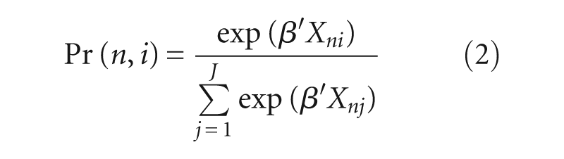
where, β denotes the parameters for each TAZ attribute. The discrete choice models developed under these assumptions are called MNL models. Models were estimated using maximum likelihood methods using BIOGEME software version 2.0 (Bierlaire, 2008).

Our descriptive analysis reveals that the sizes of projects vary quite a bit. In order to account for the size differences and the relatively greater complexity and constraints faced by developers as the magnitude of a project increases, we estimated models using project size in dwelling units as observation weight. Preliminary estimation results show much better goodness-of-fit measures for the weighted models compared with the unweighted models and parameter estimates that were more consistent with our expectations. In this paper, we reported only the estimation results from the weighted models.

Description of Explanatory Variables

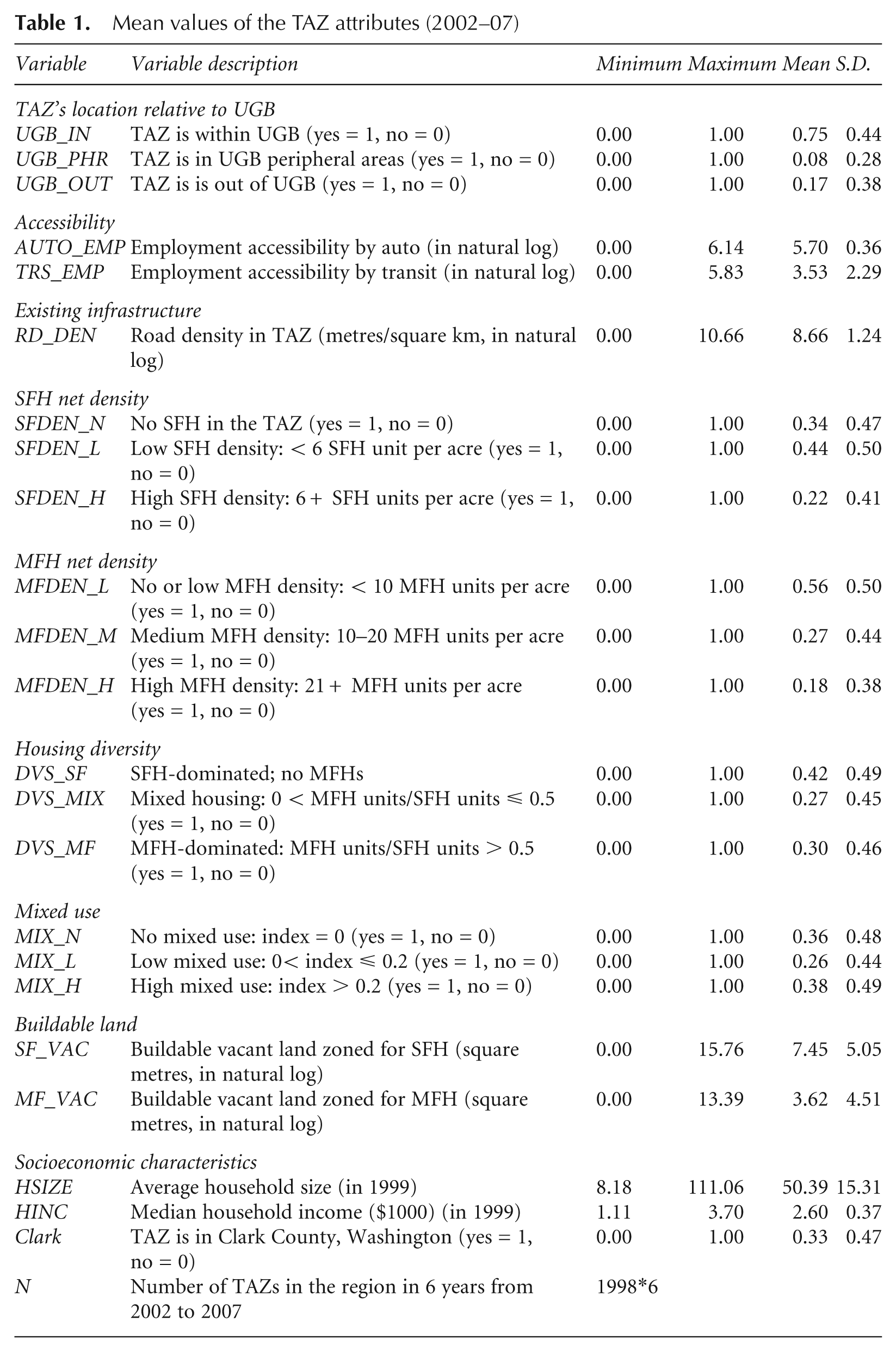
While the TAZ attribute data were available since 2000, only TAZ attributes from 2002 to 2007 were used for model estimation due to a two-year lag considered in models. Table 1 shows the descriptive statistics of TAZ attributes from 2002 to 2007.

Table 1.

Mean values of the TAZ attributes (2002–07)

Variable	Variable description	Minimum	Maximum	Mean	S.D.
TAZ’s location relative to UGB
UGB_IN	TAZ is within UGB (yes = 1, no = 0)	0.00	1.00	0.75	0.44
UGB_PHR	TAZ is in UGB peripheral areas (yes = 1, no = 0)	0.00	1.00	0.08	0.28
UGB_OUT	TAZ is is out of UGB (yes = 1, no = 0)	0.00	1.00	0.17	0.38
Accessibility
AUTO_EMP	Employment accessibility by auto (in natural log)	0.00	6.14	5.70	0.36
TRS_EMP	Employment accessibility by transit (in natural log)	0.00	5.83	3.53	2.29
Existing infrastructure
RD_DEN	Road density in TAZ (metres/square km, in natural log)	0.00	10.66	8.66	1.24
SFH net density
SFDEN_N	No SFH in the TAZ (yes = 1, no = 0)	0.00	1.00	0.34	0.47
SFDEN_L	Low SFH density: < 6 SFH unit per acre (yes = 1, no = 0)	0.00	1.00	0.44	0.50
SFDEN_H	High SFH density: 6+ SFH units per acre (yes = 1, no = 0)	0.00	1.00	0.22	0.41
MFH net density
MFDEN_L	No or low MFH density: < 10 MFH units per acre (yes = 1, no = 0)	0.00	1.00	0.56	0.50
MFDEN_M	Medium MFH density: 10–20 MFH units per acre (yes = 1, no = 0)	0.00	1.00	0.27	0.44
MFDEN_H	High MFH density: 21+ MFH units per acre (yes = 1, no = 0)	0.00	1.00	0.18	0.38
Housing diversity
DVS_SF	SFH-dominated; no MFHs	0.00	1.00	0.42	0.49
DVS_MIX	Mixed housing: 0 < MFH units/SFH units ≤ 0.5 (yes = 1, no = 0)	0.00	1.00	0.27	0.45
DVS_MF	MFH-dominated: MFH units/SFH units > 0.5 (yes = 1, no = 0)	0.00	1.00	0.30	0.46
Mixed use
MIX_N	No mixed use: index = 0 (yes = 1, no = 0)	0.00	1.00	0.36	0.48
MIX_L	Low mixed use: 0< index ≤ 0.2 (yes = 1, no = 0)	0.00	1.00	0.26	0.44
MIX_H	High mixed use: index > 0.2 (yes = 1, no = 0)	0.00	1.00	0.38	0.49
Buildable land
SF_VAC	Buildable vacant land zoned for SFH (square metres, in natural log)	0.00	15.76	7.45	5.05
MF_VAC	Buildable vacant land zoned for MFH (square metres, in natural log)	0.00	13.39	3.62	4.51
Socioeconomic characteristics
HSIZE	Average household size (in 1999)	8.18	111.06	50.39	15.31
HINC	Median household income ($1000) (in 1999)	1.11	3.70	2.60	0.37
Clark	TAZ is in Clark County, Washington (yes = 1, no = 0)	0.00	1.00	0.33	0.47
N	Number of TAZs in the region in 6 years from 2002 to 2007	1998*6

Variables Relevant to Smart Growth Policies

The effects of the UGB can be affected by many existing location attributes. The data available for this study allow us to control the effects of some of those location attributes, such as those related to residential density and diversity, mixed land use, transport accessibility and utilisation of existing infrastructure. An important consideration of this inquiry is that being inside or outside the UGB can also capture other relevant factors that are concomitant to the UGB, such as buildable land availability, whose effect we were also able to control. What remains after controlling for these factors that we can measure, is the UGB effect which we hope to capture through parameter estimates. This effect represents policies and concomitant land use conditions and costs, such as development impact fees and taxes, and perhaps consumer demand that we were not able to measure directly and hence control. Thus, we have specified UGB dummy variables in our models which indicate whether a particular location is within the UGB, in UGB peripheral areas (including TAZs straddling the UGB border and TAZs within designated UGB expansion areas),¹ or completely outside the UGB.

Smart growth encourages travel mode transition from auto to transit and TODs. In this study, the calculation of transport accessibility was based on the modelled morning two-hour peak travel times for pairs of TAZs, utilising a static estimate of 2005 congested network travel times. The Metro travel demand model also provides 2005 estimates of employment by TAZ and by industry sector. We adapted the negative exponential travel impedance formula from Meyer and Miller (2001, p. 336)

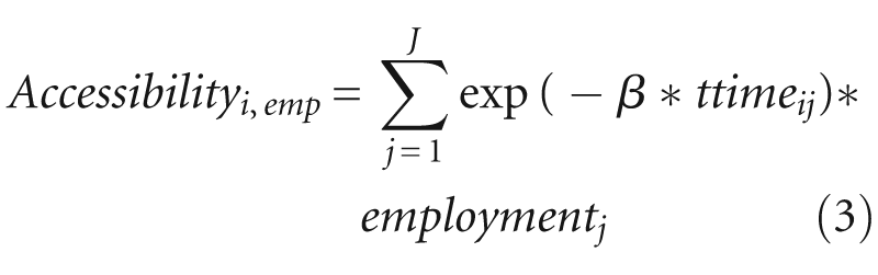
Accessibilit y_{i, emp} = \sum_{j = 1}^{J} \exp (- β * ttim e_{ij}) * employmen t_{j}

(3)

in which Accessibility_i,emp measures the employment accessibility for TAZ i; β is a parameter indicating the sensitivity of trip making to travel time; ttime_ij is the travel time from TAZ i to TAZ j; and employment_j is the number of jobs in TAZ j. With this formula, we calculated transport accessibilities by auto and transit modes for employment purpose in each TAZ. To account for their non-linear effects, both auto and transit accessibilities were used in natural log form in models. As Table 1 shows, auto provides much better travel-time weighted access to employment opportunities than transit in the region.

One important smart growth principle is to encourage new developments in locations where roads, sewers, water system and other infrastructure already exist. Haider and Miller (2004) used the length of roads to measure physical development in zones. In this study, considering that the sizes of TAZs vary a lot, we used the density of roads to represent the level of infrastructure concentration in each TAZ, which was calculated by dividing the total length of roads in a TAZ over the area of the TAZ. To account for its non-linear effect, natural log was taken when it was included in models.

Controlled Location and Socioeconomic Attributes

Besides the variables relevant to smart growth policies already discussed, there are also many other location and socioeconomic attributes that can influence home developers’ location choice. Some of them, such as residential density, housing diversity and mixed land use, are also conceptually relevant to smart growth. By including these variables in our models, we examined whether housing developments had been attracted to locations with existing location characteristics favoured by smart growth advocates in the study period.

For example, higher residential densities are generally thought to conserve land and provide critical mass for efficient transit service. In this study, we calculated TAZ-based measures of density for SFH and MFH as the total number of housing units divided by the total land area they actually occupied. Rather than using these density measures directly, we found more statistically significant correlations with location choices by grouping them into categories as indicated by Table 1.

A mix of housing types is often advocated as means of providing affordable living options to various socioeconomic strata and more equitable access to neighbourhood resources, such as schools. To measure housing diversity in each TAZ, the ratio of MFH units to SFH units in each TAZ was calculated and TAZs were grouped into three categories based on the ratio: TAZs dominated by SFHs, TAZs with mixed housing and TAZs dominated by MFHs.

Smart growth advocates mixing residential and commercial land uses to provide work and non-work opportunities within shorter travel distances, ideally fostering a sense of community and reducing auto travel. Since each TAZ’s employment accessibility has been controlled by accessibility variables, we used the ratio of the number of retail employees to the number of housing units to measure each TAZ’s mixed-use level. As shown in Table 1, based on this ratio, TAZs were categorised into three roughly even groups based on their levels of mixed use.

The availability of buildable land is a critical factor that developers have to consider when they choose locations. For SFH developments, the availability of buildable land in each TAZ is the area of vacant land zoned for low-density residential use and suitable for building houses.² For MFH developments, the availability of buildable land in each TAZ is the area of vacant land zoned for medium- and high-density residential purposes or a mixed-use purpose.³

Land price is another important factor that developers will consider when they decide locations for their projects. In this study, the only information we have about land price is the tax assessment value of land, which can be used as a rough proxy for land price. An ordinary least square (OLS) regression was run to examine the relationship between assessed land value and explanatory variables used in our models, as listed in Table 1. The regression yielded an adjusted R-squared value of about 0.74, suggesting that about 74 per cent of variations in assessed land value can be explained by other explanatory variables in the model. Another issue with the land price variable is that it might be correlated with the error component in the utility function, leading to an endogeneity problem. Therefore, the land price variable was dropped from the model.

In order to assess the effects of existing area demographics, which might have some bearing on the attractiveness of potential project sites, we included average household size and median household income, as reported in the 2000 Census for each census tract, and applied these to each TAZ. The inclusion of these two variables might also capture some characteristics of the potential consumers in the local housing market.

Besides these variables, there are still some factors such as financial incentives from local governments and corporate social responsibility that can influence developers’ location choice. However, due to data limitations, we were not able to include them in the model.

Effects of Previous Choices

A developer’s familiarity with an area based on past experience is likely to make it attractive for future work for reasons such as comfort with the local market, relationships with local contractors and government officials, and investments in local infrastructure. In addition, what appear to be multiple projects separated in time might actually be multiple phases of the same project. In this study, we hypothesise that home developers tend to locate their projects in the TAZs in which they had development activities in previous years and the TAZs that are geographically close to those TAZs. To test this hypothesis, we created variables to indicate whether alternative TAZs in a choice set were chosen by the same developer in previous years or were adjacent to TAZs chosen by the same developer in previous years. We limited our consideration to lagged variables of no more than two years in order to use as many observations as possible. Accordingly, we created four dummy variables to represent the lagged effects for developers’ location choice in year t. Auto-regressive variables AR(1) and AR(2) indicate that a TAZ in a choice set was chosen by the same developer in years t–1 and t–2 respectively. Neighbouring zone indicator variables NB(1) and NB(2) indicate that a TAZ in a choice set is adjacent to a TAZ chosen by the same developer in years t–1 and t–2 respectively. By accounting for these lagged effects, we have specified a dynamic model.

Model Results and Findings

Table 2 presents estimation results from the base models and the bi-state models for SFH and MFH developers. The base models assess to what extent SFH and MFH developer location choices were influenced by smart growth policies in the region while controlling for other site and socioeconomic variables and lagged effects of past choices. In the bi-state models, variables were interacted with a dummy variable representing TAZs in Clark County, Washington, to indicate whether there were statistically significant differences across state lines.

Table 2.

Base model and bi-state model results

	SFH developers (n = 16320)				MFH developers (n = 1138)
	Base model		Bi-state model		Base model		Bi-state model
Variables	Coefficient	S.E.	Coefficient	S.E.	Coefficient	S.E.	Coefficient	S.E.
UGB and SFH buildable land
SF_VAC	−0.1460	0.0033***	−0.1420	0.0034***			–	–
SF_VACUGB_PHR*	−0.0094	0.0030***	−0.0243	0.0040***			–	–
SF_VACUGB_PHRClark			0.0415	0.0059***	–	–	–	–
SF_VACUGB_OUT*	−0.0277	0.0033***	−0.0364	0.0043***			–	–
SF_VACUGB_OUTClark			0.0272	0.0065***	–	–	–	–
Accessibility
AUTO_EMP	−0.4040	0.0136***	−0.3990	0.0144***	−0.1190	0.1140	−0.1550	0.1070
AUTO_EMPClark*			0.1620	0.0337***			0.4500	0.1650***
TRS_EMP	−0.0217	0.0051***	−0.0461	0.0068***	−0.0127	0.0303	−0.0578	0.0327*
TRS_EMPClark*			0.0536	0.0102***			0.2170	0.0719***
Existing infrastructure
RD_DEN	−0.0811	0.0116***	−0.0864	0.0143***	0.1070	0.0542**	0.1710	0.0656***
RD_DENClark*			−0.1110	0.0232***			−0.2690	0.1040***
SFH net density
SFDEN_N					–	–	–	–
SFDEN_L	0.3200	0.0367***	0.2500	0.0488***	–	–	–	–
SFDEN_LClark*			0.2140	0.0791***	–	–
SFDEN_H	0.2840	0.0429***	0.1480	0.0554***	–	–	–	–
SFDEN_HClark*			0.5350	0.0931***			–	–
MFH net density
MFDEN_L	–	–	–	–
MFDEN_M	–	–	–	–	0.6750	0.1530***	0.6080	0.1610***
MFDEN_MClark*			–	–			0.2740	0.5190
MFDEN_H	–	–	–	–	1.1500	0.1560***	1.1900	0.1630***
MFDEN_HClark*			–	–			−0.5770	0.5500
Housing diversity
DVS_SF	–	–	–	–
DVS_MIX	−0.1070	0.0249***	0.1700	0.0360***	−0.1650	0.1880	0.0218	0.2310
DVS_SFClark*			−0.5530	0.0525***			−0.6590	0.5200
DVS_MF	−0.1430	0.0280***	0.0406	0.0375	0.1710	0.1900	0.3680	0.2300
DVS_MFClark*			−0.0776	0.0619			−0.4400	0.5700
Mixed use
MIX_N	–	–	–	–	–	–	–	–
MIX_L	0.2230	0.0222***	0.2340	0.0298***	0.6740	0.1120***	0.8630	0.1490***
MIX_LClark*			0.0201	0.0458			−0.7660	0.2590***
MIX_H	0.1940	0.0240***	0.2310	0.0306***	0.3950	0.1100***	0.5710	0.1480***
MIX_HClark*			0.0063	0.0540			−0.6870	0.2520***
MFH buildable land
MF_VAC	–	–	–	–	0.2130	0.0101***	0.2180	0.0120***
MF_VACClark*			–	–			−0.0227	0.0224
Socio-economic attributes
HSIZE	0.8700	0.0336***	0.7950	0.0347***	−1.4000	0.0913***	−1.3800	0.0937***
HINC					0.0052	0.0025**	0.0057	0.0025**
AR(1)	4.7900	0.0460***	4.7900	0.0461***	5.0900	0.1510***	5.0800	0.1510***
NB(1)	0.9010	0.0571***	0.9040	0.0571***	2.0900	0.2140***	2.0900	0.2130***
AR(2)	0.7440	0.0715***	0.7470	0.0714***	0.8210	0.3180***	0.8290	0.3170***
NB(2)	0.7720	0.0610***	0.7590	0.0610***	1.4500	0.2580***	1.4500	0.2580***
Number of parameters	17		28		16		26
Null log likelihood	−63 844		−63 844		−8 649		−8 649
Final log likelihood	−40 978		−40 806		−6 873		−6 848
Rho squared	0.358		0.361		0.205		0.208
Adjusted Rho squared	0.358		0.360		0.203		0.205
Weighting variable	Project size		Project size		Project size		Project size

Notes: * significant at the 10 per cent level; ** significant at the 5 per cent level; *** significant at the 1 per cent level.

UGB

As mentioned earlier, for each SFH project, only TAZs with enough buildable vacant land were considered as eligible alternatives in its choice set. In SFH models, UGB dummy variables were interacted with the amount of buildable land in each TAZ to test how their locations relative to the UGB affected the chances of buildable land being chosen by SFH developers.

Estimation results of the base model show that for TAZs within the UGB, SFH developers tend to choose TAZs with less amount of buildable land. With vacant land within the UGB as the reference, vacant land in UGB peripheral areas and outside the UGB is less likely to be chosen by SFH developers, indicating that the UGB in the Portland region has successfully reduced SFH developments in urban peripheral and rural areas. However, the bi-state model shows that, compared with SFH developers on the Oregon side, SFH developers in Clark County, Washington, are more likely to choose vacant land in peripheral areas and outside the UGB, suggesting that the UGB in the three Oregon counties is more effective in containing SFH developments within the UGB. This may reflect a more lenient growth management policy framework in Clark County, Washington, compared with the three Oregon counties. Since most MFH developments were within the UGB, UGB dummy variables were not included in MFH models.

Auto and Transit Accessibility

As shown in Table 2, the effects of both auto and transit accessibilities for employment are negative for SFH developments. This can be interpreted to suggest that SFH developers in the Portland metropolitan area still show a propensity to locate away from major employment centres, especially the Portland city centre, which has the highest auto and transit accessibilities for employment purposes. The SFH bi-state model shows that SFH developers in Clark County, Washington, are more likely to choose locations with better auto and transit accessibilities than those in Oregon. This can be attributed to the fact that the city of Vancouver, the employment centre of Clark County, Washington, has more buildable land for SFH developments than the city of Portland.

The base model for MFH developers shows that they are not sensitive to auto and transit accessibilities. However, the bi-state model suggests that MFH developers in Clark County, Washington, are more likely to choose locations with better auto and transit accessibilities, which tend to be TAZs in the city of Vancouver. This might reflect the fact that MFH projects in the three Oregon counties are more dispersed, while MFH developments in Clark County, Washington, are concentrated in the city of Vancouver.

Existing Infrastructure Concentration

Using road density as a proxy for development-supportive existing infrastructure, we tested the hypothesis that smart growth policies encourage more efficient use of existing infrastructure. Model results indicate that SFH developers in both states are more likely to choose locations with less infrastructure concentration, consistent with the finding that SFH developments tend to locate away from major employment centres in the region. However, compared with their counterparts in Clark County, Washington, Oregon SFH developers tend to choose locations with higher infrastructure concentration. This confirms the finding that SFH developers on the Oregon side are more likely to choose vacant land within the UGB, which tends to have higher infrastructure density than vacant land in UGB peripheral areas or outside the UGB.

Different from SFH developers, MFH developers are more likely to choose locations with higher infrastructure density. However, the MFH bi-state model shows that this only applies to MFH developers on the Oregon side. MFH developers in Clark County, Washington, tend to choose locations with lower infrastructure density. This contrast suggests that smart growth policies in Oregon have been more effective in encouraging new high-density developments in locations with higher existing infrastructure concentration.

Site Characteristics and Socioeconomic Variables Controlled

Residential density

The existing density of SFH in units per acre was found to have a significant, positive effect on the location preference of SFH developments. Relative to the reference case of zero existing SFH units, SFH developers are more likely to choose locations with some existing SFH units. However, SFH developers in Oregon and Washington show different tastes in existing SFH density. In the three Oregon counties, SFH developers prefer locations with low-density SFHs, but those in Clark County, Washington, show a preference for locations with high-density SFHs. This may be a sign of SFH densification in Clark County, Washington.

Our model results show that MFH developers prefer locations with some existing MFH units, especially locations with high-density MFHs, and the differences between developers in Oregon and Washington are not statistically significant.

Housing diversity

Regarding housing diversity, our base model results indicate that SFH developers still prefer locations without any MFHs, rather than those with mixed housing. In the bi-state model, however, SFH developers in the two states show different tastes in housing diversity. In the three Oregon counties, the preference would be for developing in ‘mixed housing’ zones, followed by ‘SFH-dominated’ and ‘MFH-dominated’ zones. In Clark County, the net effect of the parameter estimates reveals a preference for ‘SFH-dominated’ and ‘MFH-dominated’ zones followed by ‘mixed housing’ zones. The seeming ambiguity of the Clark County results might reflect a less mature growth management system in which there is an existing shortage of mixed housing areas.

Both the MFH base and bi-state models show that MFH developers in both states are not sensitive to housing diversity in zones.

Mixed use

Using ‘No mixed use’ TAZs as the reference case, the base model suggests that SFH developers are more likely to choose TAZs with somewhat mixed use and bi-state model results show that this is true for SFH developers in both Oregon and Washington.

For MFH developers, our base model results show that they also prefer locations with mixed use, especially zones with low-level mixed use. The bi-state model, however, shows significant offsetting negative parameters for Clark County. The net effect is that MFH developers in Clark County are more likely to choose zones with low mixed use, followed by zones with no mixed use and, finally, zones with high mixed use. Recent efforts to guide growth into a mixed-use scenario in Washington is in its early stages; therefore, lacking a great deal of existing highly mixed-use areas, new housing developments are being built in areas with low or no mixed use.

Buildable land

In the SFH models, the buildable land variable is interacted with UGB dummy variables and the model results were discussed earlier. For MFH developments, the supply of vacant developable land in a TAZ is an important attractor for MFH developments and this is evident in our models by the very strong, significant positive parameter estimates of MFH-zoned vacant land. The MFH bi-state model shows that the difference of marginal utility of each additional vacant square metre is statistically insignificant in the two states.

Socioeconomic variables

Average household size and median household income at the census-tract level were used to represent socioeconomic characteristics of zones and potential local housing market. Since the effect of the household income variable was inconsistent across different numbers of draws while sampling alternative zones for SFH developers, it was dropped from the SFH models. Model results of the household size variable show that it has a very significant positive effect on SFH developments, but a very significant negative effect on MFH developments, which makes sense since the MFH market in the Portland region tends to meet the demand of small-size households, such as young couples without children. Model results suggest a positive effect of household income on MFH developments, indicating that MFH developers prefer zones with higher median household income.

Lagged Effects of Previous Choices

The estimation results on lagged effects on SFH and MFH developers are similar and quite intuitive. As shown in Table 2, if a developer was active within the previous two years, there is a significant positive effect of locating the current project in the same TAZ as the previous project, or in a neighbouring TAZ. The effects lessen somewhat going from a one-year lag to a two-year lag and are greater for the same zone (AR) than for a neighbouring zone (NB). The magnitude and significance of these variables make them the strongest predictors in the entire specification. This confirms the finding by Haider and Miller (2004) that developers tend to focus on locations in which they have built before. In addition, lagged effect variables might also capture some factors that influence developers’ location choice but are missed from our models.

Conclusions

The developer project location choice models developed in this study show that home developers in the Portland metropolitan area are sensitive to most smart growth policies being implemented in the region, but they react to them differently across the border between Oregon and Washington. In addition, SFH and MFH developers show different preferences for location attributes.

On the Oregon side of the Portland metropolitan area, everything else equal, there is a preference for developing SFH units on vacant land within the UGB, rather than that in UGB peripheral areas and outside the UGB. This lends supports for the argument that Portland’s UGB has successfully reduced urban sprawl in the region. On the Washington side, developers also show a propensity to avoid developing SFH units on vacant land outside the UGB, but they show a preference for vacant land in UGB peripheral areas over those within the UGB, which may reflect a market segment preference for moderately priced houses with large-size land lots and may be largely the collective outcome of many one-time private developers who build a single residence on a large lot in rural areas in Clark County, Washington. Compared with the long history of urban growth management in Oregon, the implementation of Washington’s GMA and its recent efforts to guide growth into the UGB are in their early stages.

SFH and MFH developers in both states show a strong propensity to locate away from major employment centres with better transport accessibility for employment purposes. Compared with developers on the Oregon side, developers in Clark County, Washington, are more likely to choose locations with better transport accessibility, possibly due to the larger amount of buildable land in the city of Vancouver.

Both SFH and MFH developments in the three Oregon counties are more likely to be in zones with higher infrastructure concentration than their counterparts in Clark County, Washington. In Oregon, state legislation requires consistency between transport and land use plans and the Oregon Department of Transportation is involved in reviewing plan amendments; thus the adequate provision of infrastructure is assured.

In both states, SFH developers seem to respond positively to existing location attributes that follow smart growth principles in terms of encouraging home developments at higher densities, providing a mix of housing types and encouraging mixed-use development. One exception is that it seems that SFH developers in Clark County, Washington, show a tendency to avoid zones with mixed housing. Our interpretation is that, compared with the three Oregon counties, Clark County has fewer existing neighbourhoods with mixed housing and, due to its suburban and rural lifestyles, the market potential for mixed housing projects is limited.

In terms of MFH, in both states the development preferences seem to favour existing locations with higher MFH density. At the same time, we found that, compared with their counterparts in Clark County, MFH developers in the three Oregon counties are more likely to choose locations with mixed land use.

In terms of future research, conducting in-depth interviews and structural surveys on housing developers will be helpful to understand how developers view smart growth policies and what role those policies play when they choose project locations. The models developed in this study implicitly assume taste homogeneity for location attribute preferences and we intend to examine to what extent taste variation plays a role in location choice decisions. Finally, future research should also consider the impacts of smart growth policies on commercial property developments.

Footnotes

Acknowledgements

The authors are thankful to three anonymous referees and Joe Broach for their constructive comments and suggestions. They are also thankful to Metro for their data support.

Notes

Funding Statement

This research received no specific grant from any funding agency in the public, commercial or not-for-profit sectors.

References

Abbott

(1997) The Portland region: where city and suburbs talk to each other and often agree, Housing Policy Debate, 8(1), pp. 11–51.

Abbott

(2002) Planning a sustainable city: the promise and performance of Portland’s urban growth boundary, in: Squires

G. D.

(Ed.) Urban Sprawl: Causes, Consequences, and Policy Responses, pp. 207–235. Washington, DC: Urban Institute.

Bierlaire

(2008) Estimation of discrete choice models with BIOGEME 1.8 ( http://biogeme.epfl.ch ).

Downs

(2005) Smart growth: why we discuss it more than we do it, Journal of the American Planning Association, 71(4), pp. 367–378.

Haider

Miller

E. J.

(2004) Modeling location choices of home builders in the greater Toronto area, Transportation Research Record, 1898, pp. 148–156.

Jun

M. J.

(2004) The effects of Portland’s urban growth boundary on urban development patterns and commuting, Urban Studies, 41, pp. 1333–1348.

McFadden

(1978) Modeling the choice of residential location, Transportation Research Record, 673, pp. 72–77.

Metro (1992) Metro charter. As adopted in November 1992 and amended in November 2000 (http://www.oregonmetro.gov/index.cfm/go/by.web/id=629; accessed 2 March 2010).

Metro (1995) 2040 growth concept ( http://www.oregonmetro.gov/index.cfm/go/by.web/id=29882 ; accessed 3 March 2010).

10.

Meyer

M. D.

Miller

E. J.

(2001) Urban Transportation Planning. New York: McGraw-Hill.

11.

Nelson

A. C.

Moore

(1993) Assessing urban growth management: the case of Portland, Oregon, the USA’s largest urban growth boundary, Land Use Policy, 10(4), pp. 293–302.

12.

Nerella

Bhat

C. R.

(2004) Numerical analysis of effect of sampling of alternatives in discrete choice models, Transportation Research Record, 1894, pp. 11–19.

13.

O’Connell

(2009) The impact of local supporters on smart growth policy adoption, Journal of the American Planning Association, 75(3), pp. 281–291.

14.

Richardson

H. W.

Gordon

(2001) Sustainable Portland? A critique, and the Los angles counterpoint. Paper presented at the ACSP Conference, Cleveland, OH, November.

15.

Song

Knaap

G. J.

(2004) Measuring the effects of mixed land uses on housing values, Regional Science and Urban Economics, 34, pp. 663–680.

16.

Train

K. E.

(2003) Discrete Choice Methods with Simulation. New York: Cambridge University Press.

17.

US Bureau of the Census (2000) Census 2000. Census Bureau, US Department of Commerce, Washington, DC.

18.

Weitz

(1999) Sprawl Busting: State Programs to Guide Growth. Chicago, IL: Planners Press.