
Abstract
Little appears to be known about the value of urban green spaces (tree canopy cover and grassy areas) in a Mediterranean climate, or in relation to multifamily buildings. This study starts addressing this gap by quantifying the impact of urban green spaces on the value of 1197 multifamily buildings sold in 2003/04 in Los Angeles, California. To assess the robustness of the results, a spatial Durbin model is contrasted with a geographically weighted regression model and an extensive sensitivity analysis is conducted. It is found that increases in grassy areas either on the parcels of multifamily buildings or in their vicinity (200 metres outward from each parcel boundary) would typically not enhance their value and neither would more parcel tree canopy cover (TCC); by contrast, most multifamily properties would benefit from an increase in vicinity TCC. These results have implications for tree planting programmes that rely heavily on private property owners.
The best time to plant a tree was 20 years ago. The next best time is now (Chinese proverb).
1. Introduction
Many cities around the United States appear to have embraced this old Chinese proverb, as urbanites seem increasingly convinced of the many benefits of trees and green spaces. Indeed, they beautify neighbourhoods and provide habitats for many species. Shade from trees decreases energy use, which helps to reduce the urban heat island effect. Trees also improve urban air quality, mostly by intercepting particulate matter and by capturing ozone as well as nitrogen dioxide (Miller, 1997) and they remove some carbon dioxide from the atmosphere. Finally, trees help to control erosion by limiting water runoff. As a result, many cities, including Baltimore, Denver, Los Angeles and New York have undertaken large urban tree planting programmes.
As emphasised in Conway et al. (2010), however, the dearth of empirical research on the amenity value of neighbourhood green spaces is problematic for justifying large public tree planting programmes in periods of stressed local budgets. Furthermore, our review of the literature revealed that the benefits of trees have been assessed only for a few ecosystems and mostly in relation to single-family detached houses. Little appears to be known about the impact of green spaces on the value of multifamily buildings and, with the exception of Conway et al. (2010), we found no published paper on the value of urban green spaces in Mediterranean environments like southern California.
In this context, our paper makes two contributions. First, it quantifies the impact of local land cover on the value of multifamily buildings in Los Angeles (LA). This is especially important because LA residents of multifamily buildings are often disadvantaged economically and belong to minority groups. Secondly, our econometric analysis contrasts a spatial Durbin model with a geographically weighted regression model to improve our understanding of how values from urban green spaces vary spatially. Improving the handling of the omitted variable bias (resulting from local omitted variables) and spatial autocorrelation enables us to obtain more robust results.
We find that increases in grassy areas either on parcels of multifamily buildings or in their vicinity (200 metres outward from each parcel boundary) would typically not enhance their value and neither would more parcel tree canopy cover (TCC); by contrast, most multifamily properties would benefit from an increase in vicinity TCC.
In the next section, we provide some background on the economic valuation of urban green spaces with an emphasis on hedonic studies. In section 3, we present our data and in section 4 we introduce our methodology. Section 5 discusses our results and section 6 examines their implications for tree planting in Los Angeles. The last section summarises our conclusions.
2. Background and Literature Review
Different methods have been employed to estimate the value of urban green spaces. A number of papers (see Brander and Koetse, 2007, for references) have relied on contingent valuation. However, this method relies on stated preferences that may not translate into actual behaviour. An alternative is the travel cost method, but, with the exception of Dwyer et al. (1983), it has not been used for valuing urban green spaces because it is not thought to work well for neighbourhood recreational resources (More et al., 1988). Others have valued urban trees based on the benefits and costs of the ecological services they provide (for example, see McPherson et al., 2005; Nowak et al., 2007). This is clearly useful for policy analysis, but it requires detailed data on tree populations and community forestry expenditures that are often unavailable.
In this paper, we rely instead on the hedonic pricing method, which explains the price of a product by its characteristics using observed market behaviour (Rosen, 1974). This widely popular approach (see Sirmans et al., 2006) was first applied to urban forests in the 1970s (Payne, 1973; Morales et al., 1976). Early papers relied on ad hoc samples analysed via ordinary least squares (OLS) and typically found that trees increase the value of single-family detached houses. According to Morales (1980), for example, good tree cover could add 6 per cent to the value of a house.
In the past decade, many published hedonic studies of urban trees have analysed larger datasets of single-family detached houses using OLS with time and sub-market dummy variables and they have considered spatial autocorrelation. For example, Des Rosiers et al. (2002) examined the impact of trees and landscaping on 760 homes sold between 1993 and 2000 around Québec City (Canada). They found that each percentage difference in tree cover with a property’s immediate neighbours raises its value by 0.2 per cent. Kestens et al. (2004), who studied 2740 houses in the same area for different years (1986/87 and 1993–96), concluded that an increase of 10 per cent in mature trees within 100 metres of a home raises its value by 1 per cent. Mansfield et al. (2005) analysed 11 200 homes sold in 1996–98 in the Research Triangle Region (North Carolina, USA). They reported that increasing parcel forest cover by 10 per cent adds less than $800 to property values, which is small compared with other published estimates. More recently, Kong et al. (2007) considered a wider set of urban amenities for Jinan City (China); they found that a higher forest scenery index, accessibility to parks and green plazas, and a higher percentage of urban green space significantly increase property values.
Two papers that analyse data from Portland, Oregon (USA) stand out. The first one (Netusil et al., 2010) includes a second-stage hedonic analysis, which is uncommon. After examining 30 015 properties sold in 1999–2001, the authors reported that the mean canopy cover within one-quarter of a mile of a property is worth between 0.75 and 2.52 per cent of its mean sale price. In another recent paper, Donovan and Butry (2010) modelled the impact of trees and time-on-market on the value of 3479 properties sold in 2006/07. They found that trees add on average $8870 to sales price and reduce time-on-market by 1.7 days.
A couple of published papers have relied on spatial hedonic models. Sander et al. (2010) estimated a spatial error model with monthly and school district dummy variables on 9992 homes sold in 2005 in two Minnesota (USA) counties. According to their results, a 10 per cent increase in tree canopy cover within 100 metres increases the average home price by $1371. Conway et al. (2010) considered instead a spatial lag model to examine 260 homes sold in 1999/2000 in Los Angeles, California (USA). According to their results, a 1 per cent increase in green spaces 200–300 metres from single-family properties raises their value by 0.07 per cent.
Other hedonic studies have investigated the value of urban trees on the rent of commercial buildings (Laverne and Winson-Geideman, 2003) and how distance to urban parks impacts house prices (see Cho et al., 2006, and references herein). For an overview of older hedonic papers, see Sander et al. (2010). Except for Conway et al. (2010), however, none of the studies referenced has considered urban green spaces found in the Mediterranean climate that characterises Los Angeles and many developing megacities. Anderson and Cordell (1988), for example, emphasised that their findings are limited to the eastern part of the US. Moreover, we found only two published hedonic studies dealing with multifamily housing (Fisher et al., 2005; Sun and Yu, 2005) but they do not consider the value of urban land cover.
The multifamily housing market, especially for buildings with five or more units, is distinctly different from the single-family residential market. Larger multifamily buildings are generally considered to be commercial properties (US Census Bureau, 2005). Their owners often use these properties to generate rent income and they do not reside in them. Multifamily building residents are also more likely to be economically disadvantaged and to belong to minority groups (Goodman, 1999). As a result, urban trees and green spaces may impact the value of multifamily properties differently than they do single-family detached buildings. In this study, our starting hypothesis is that trees and irrigated grass are positive amenities that enhance the value of multifamily buildings. We test this hypothesis on measures of green spaces both on the parcels of multifamily buildings and in their vicinity.
3. Data
Our study analyses the price of multifamily buildings sold in 2003 and 2004 in the city of Los Angeles, California. Table 1 defines our variables and presents summary statistics.
Descriptive statistics of variables in this research (N = 1197 households)
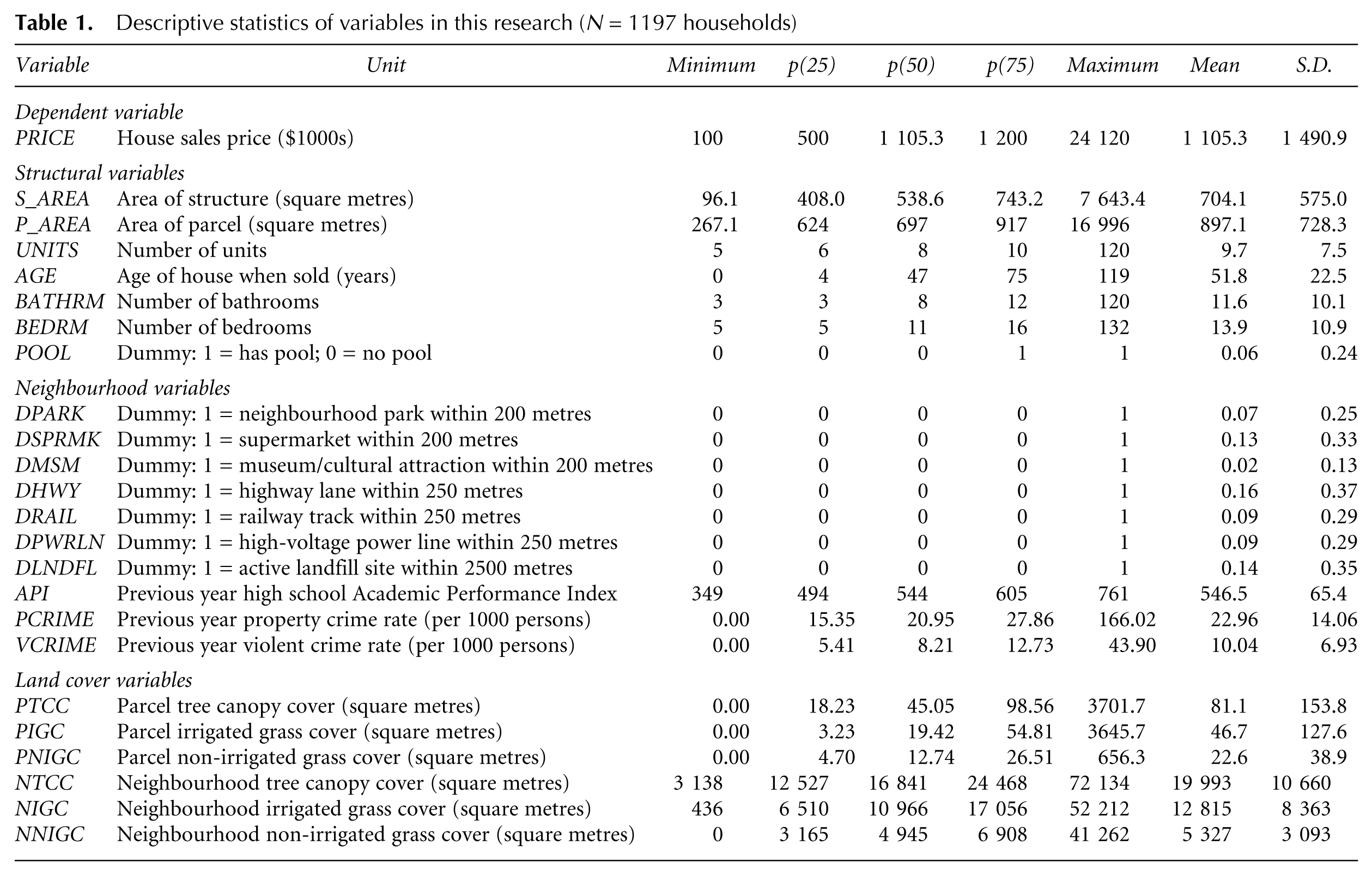
We purchased our housing data from DataQuick Information Systems. 1 Each building was mapped using the ArcGIS software with reference to the Los Angeles County Parcel Boundary Map from the Assessor’s Office, because this approach proved more accurate than relying on street addresses. Available structural variables include age, parcel area, structural square footage, number of units, number of bathrooms, number of bedrooms and presence of a pool.
In addition, neighbourhood variables were collected from different sources. ESRI Inc. (the developer of ArcGIS) gave us coastlines, parks and highways data. Several public agencies kindly shared their data with us, including the California Department of Transportation (location of high voltage transmission lines and railroad tracks), the Los Angeles County Sanitation District (landfill locations), the Los Angeles Police Department (crime data) and the Los Angeles Unified School District (High School Academic Performance Index data). We also obtained from Zillow Inc. the boundaries of their Los Angeles neighbourhoods. Zillow developed its neighbourhoods in consultation with the Los Angeles chamber of commerce, tourism and convention boards, real estate agents and community members. We then calculated distances from each multifamily building to the nearest local features of interest (such as parks or museums) and to the coastline using geographical information system (GIS) software.
The variables of primary interest to this study are land cover variables. We relied on a unique dataset created by McPherson et al. (2007), who generated a high-resolution (2 feet) land cover map that provides information about tree canopy cover (TCC), irrigated grass cover (IGC), non-irrigated grass cover/bare soil (NIGC) and impervious surfaces from high-resolution QuickBird remote sensing data and aerial photographs of the city of Los Angeles. Their work showed that 21 per cent of the city of Los Angeles is covered by trees, while IGC and NIGC account respectively for 12 per cent and 6 per cent of the city’s area. As expected, TCC is strongly related to land use: low-density residential land uses have the highest TCC (31 per cent), while industrial and commercial land uses have the lowest TCC (3–6 per cent).
To capture the impact of land cover on housing values, we created two sets of variables. The first set comprises the areas of TCC, IGC and NIGC on the parcel of each multifamily building in our dataset. The second set includes similar land covers variables measured in an area 200 metres outward from each parcel boundary. These ‘vicinity’ variables are designed to capture land use near each multifamily property; we chose 200 metres because it reflects how far most Americans are willing to walk away from their house (Krizek and Johnson, 2006). Since our best model includes the logarithm of these land cover variables, we added 1 square metre to land cover variables that equal zero to avoid losing valid observations.
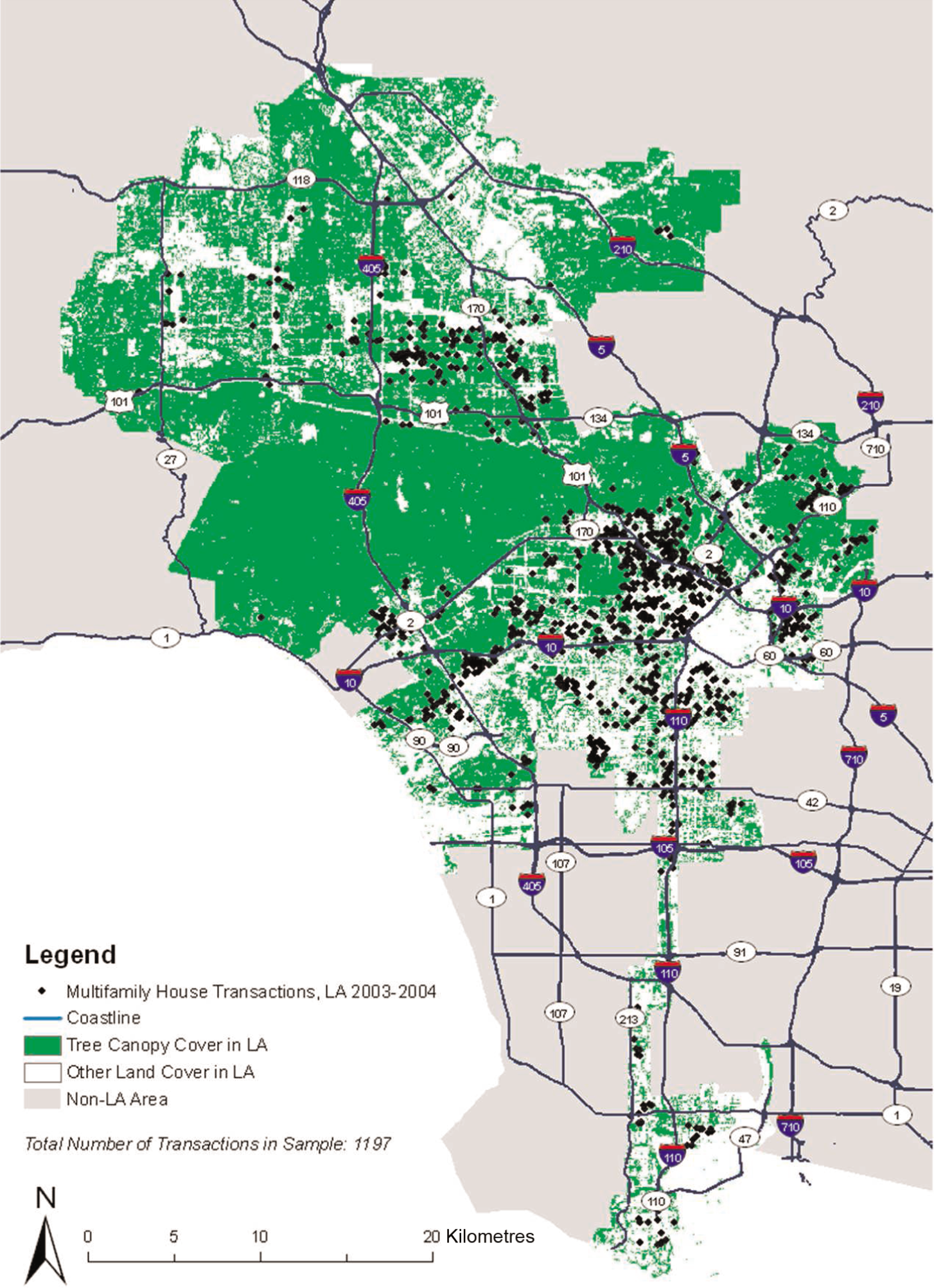
Our initial DataQuick dataset had 2909 transactions. We discarded 1291 observations with missing variables (including 1003 properties with no sales price), 318 observations with unlikely structural characteristics and 85 observations whose price per square foot was excessively high or low, based on local real estate websites. Generally, buildings with missing sales price had more units and were more likely to have a pool, but they were located in socioeconomic areas similar to the rest of our dataset, so their absence should not bias our results. Finally, to prepare for our spatial hedonic models, we dropped 18 observations that were alone in their Zillow neighbourhood. These steps left us with 1197 observations for modelling (see Figure 1).
Tree canopy cover and location of multifamily buildings sold in 2003/04 in Los Angeles, CA.
4. Methodology
4.1 Overview
Following the standard hedonic framework (Rosen, 1974), we explain the market price

The partial derivative of f with respect to a characteristic is an implicit price that represents marginal willingness to pay for that characteristic.
To be valid, Rosen’s (1974) framework requires perfect competition and market equilibrium, perfect information for buyers and sellers, and a continuum of products. Some of these conditions may not be met in practice. Fortunately, Bajari and Benkard (2005) showed that perfect competition, perfect information and a continuum of products are not necessary for the hedonic pricing method to be valid. Moreover, Maclennan (1977) argued that market equilibrium can be assumed in the absence of severe shocks, which is the case here. Meese and Wallace (1997) further found that real estate markets typically adjust quickly to small shocks, so we assume that the 2003/04 Los Angeles housing market was in equilibrium.
Unfortunately, economic theory provides little guidance for choosing the functional form of hedonic models. In a recent paper, Kuminoff et al. (2010) recommend flexible approaches that include spatial fixed effects, temporal controls and Box–Cox transforms. However, the Box–Cox transformation is not readily available for the spatial models we considered (Kim et al., 2003). In addition, spatial fixed effects models are not ideal here because their fine-scale implementation requires many degrees of freedom (Redfearn, 2009). To guide our model selection, we inspected graphically the relationship between sales price and the continuous explanatory variables in our dataset, which suggested a log–log model. We also explored log–linear models, which we compared with log–log models with the same variables using the Akaike and the Bayesian information criteria (AIC and BIC).
One of the main challenges to overcome when estimating a hedonic model is omitted variables. Indeed, it is well known that omitting an important variable leads to biased and inconsistent estimators if this omitted variable is correlated with the included independent variables (Greene, 2007). As shown by Case (1991), omitted variables may be spatially correlated and thus create spatial autocorrelation in the error terms of hedonic models; examples include local climate and neighbourhood quality.
Even the most extensive data collection efforts cannot remove the threat of omitted variable bias. One common remedy is to estimate spatial hedonic models; following Brasington and Hite (2005) and Pace and LeSage (2008), we adopted the spatial Durbin model (SDM). Another possibility is to estimate a geographically weighted regression model (GWRM). Both control for spatial dependence, but the flexible functional form of a GWRM might be better suited to capture the diversity and the complexity of Los Angeles’ sub-markets (Redfearn, 2009). For an in-depth discussion of other econometric issues related to hedonic models, see Taylor (2008).
4.2 The Spatial Durbin Model (SDM)
The spatial Durbin model (Anselin, 1988; Kim et al., 2003) is more general than the spatial autoregressive model and the spatial error model, both of which can be obtained by imposing restrictions (Brasington and Hite, 2005). Let M, N and K respectively designate our sample size, the number of explanatory variables (including an intercept) and the number of explanatory variables with spatial lags. Our SDM can then be written
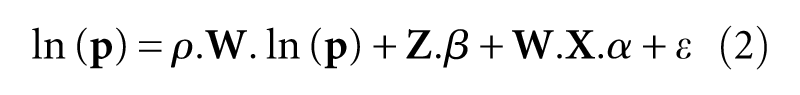
where, ln(
The term ρ·
Real estate prices can also depend on non-monetary attributes of neighbouring properties. For example, property values go down when a nearby house has poorly maintained landscaping or graffiti on its walls. This spillover effect is captured by the spatial lag term
To assess the influence of
For our first weight matrix, neighbours of a property are in the same Zillow neighbourhood and they have equal weights. Our second weight matrix also relies on Zillow neighbourhood but a weight is inversely proportional to the squared distance between a property and its neighbour. For our third weight matrix, neighbours of a property share a Delaunay triangle (Pace and Le Sage, 2003) with it and have equal weights. Since parameter estimates were very similar with all three weight matrices, we present results only for the first one.
To interpret equation (2), we move all price terms to the left side, left-multiply throughout by
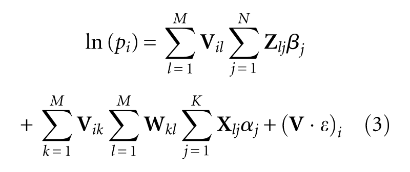
where, the subscript ij on a matrix denotes the component on its ith row and jth column, and
From equation (3), we see that the elasticity of price varies with each observation. Simple derivations
2
show that the elasticity of price of observation i with respect to continuous explanatory variable

We can interpret
For our first weight matrix,
Arraiz et al. (2010) showed that heteroscedasticity could cause parameters obtained by maximum likelihood to be inconsistent for a wide class of spatial models that includes the SDM, so with Kelejian and Prucha (2010, and references therein) they proposed instrumental variables and generalised-method-of-moments (GMM) techniques that yield consistent model parameters. We therefore investigated the presence of heteroscedasticity and conducted a careful analysis to assess the validity of our results.
4.3 Geographically Weighted Regression Model (GWRM)
To gauge the robustness of our results, we also considered a geographically weighted regression model (GWRM), which entails estimating a weighted least-squares model for each observation with a diagonal weight matrix

where, now
To calculate the diagonal term

where,
Some researchers (for example, Cho et al., 2006) set to zero the weights of observations beyond b. Although this approach reduces the computational burden, it is unsuitable here because it would produce a weight matrix with few observations in some areas outside downtown Los Angeles, which would compromise the precision of our estimates.
5. Results and Discussion
Our results were obtained using Stata 11.2. For the SDM, we relied on “spmlreg” (Jeanty, 2010) complemented with “spreg” (Drukker et al., 2011) for robustness checks and, for the GWRM, we used “gwr” (Pearce, 1999). In our discussion, we mention all significant digits in order to connect the text to Table 2 without implying great precision.
Modeling results (N = 1197 households)
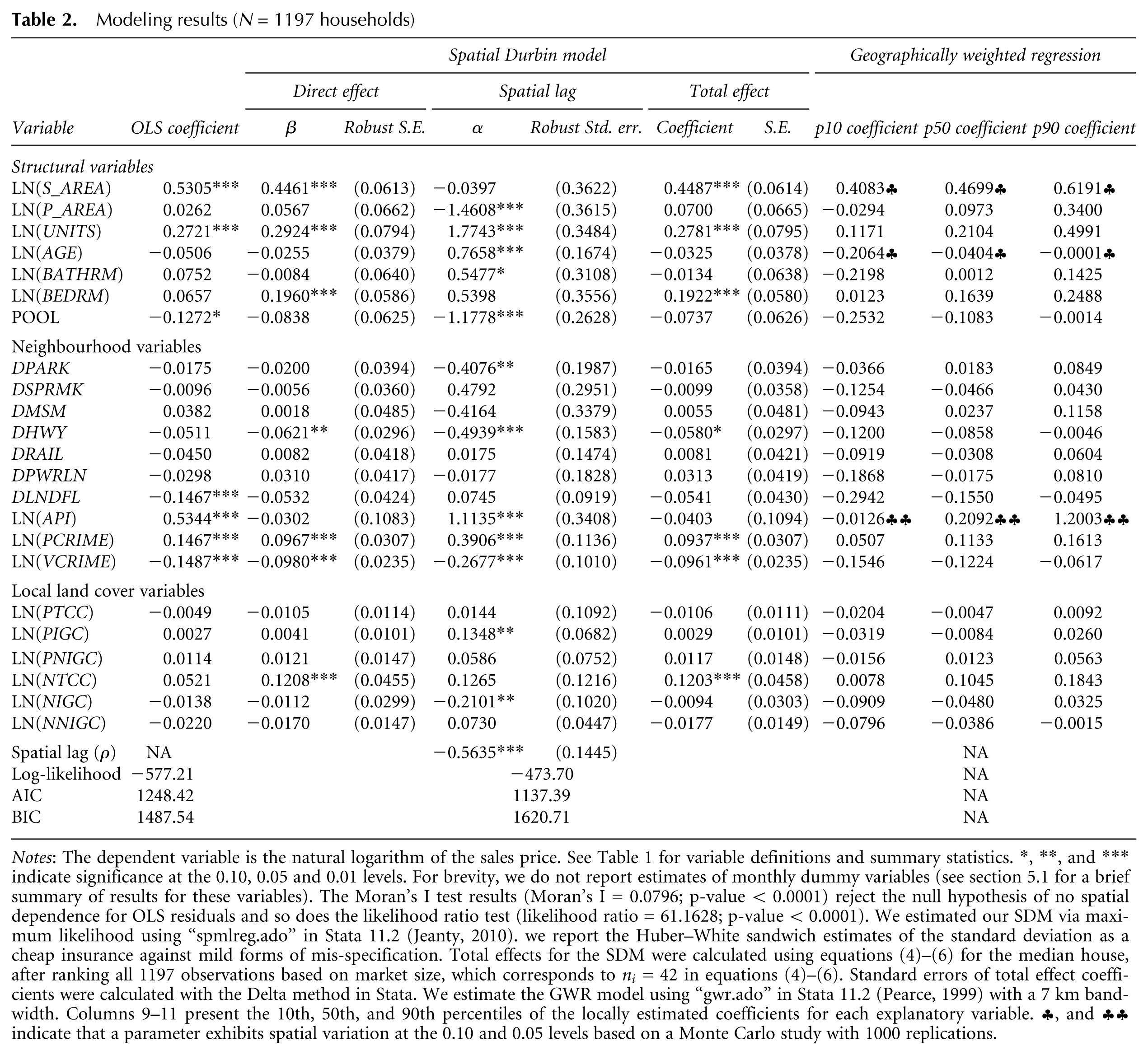
Notes: The dependent variable is the natural logarithm of the sales price. See Table 1 for variable definitions and summary statistics. *, **, and *** indicate significance at the 0.10, 0.05 and 0.01 levels. For brevity, we do not report estimates of monthly dummy variables (see section 5.1 for a brief summary of results for these variables). The Moran’s I test results (Moran’s I = 0.0796; p-value < 0.0001) reject the null hypothesis of no spatial dependence for OLS residuals and so does the likelihood ratio test (likelihood ratio = 61.1628; p-value < 0.0001). We estimated our SDM via maximum likelihood using “spmlreg.ado” in Stata 11.2 (Jeanty, 2010). we report the Huber–White sandwich estimates of the standard deviation as a cheap insurance against mild forms of mis-specification. Total effects for the SDM were calculated using equations (4)–(6) for the median house, after ranking all 1197 observations based on market size, which corresponds to
5.1 Results for the Spatial Durbin Model (SDM)
To check the homoskedasticity assumption, we first graphed SDM residuals versus our estimated dependent variable but did not detect any pattern. In the spirit of the Breusch–Pagan LM test (Greene, 2007), we then regressed the squared residuals on our independent variables. We obtained a low R2 (= 0.0587) and could not reject the null hypothesis that model parameters are jointly 0 (at 1 per cent) based on an F-test. In addition, we estimated a Cliff–Ord model (Anselin, 1988) with the same explanatory variables as our SDM model and with spatial lags for the dependent variable and for the error terms, which gave very similar results via maximum likelihood and heteroscedasticity-robust GMM (Drukker et al., 2011). Finally, we added a spatially lagged error to equation (2) and found that it is not statistically different from 0. All these tests suggest that heteroscedasticity is not a problem here and that the SDM is a sensible choice.
Results are summarised in Table 2. For brevity, we do not report estimates of monthly dummy coefficients. With the exception of the February 2003 coefficient, they are positive and they tend to increase over time. When we discuss the significance of SDM parameters, we refer to total effects, for which standard errors were calculated via the Delta method (Greene, 2007).
Structural and neighbourhood variables
Results for structural and neighbourhood characteristics appear reasonable and generally conform to our expectations. The sales price of a multifamily property increases by 0.4487 per cent for every 1 per cent increase in structural area, 0.2781 per cent for every 1 per cent increase in the number of units and 0.1922 per cent for every unit increase in the number of bedrooms. These parameters are all statistically significant (p-value <0.01) and their distributions are clustered around their means. Coefficient estimates of other structural variables appear reasonable but they are not statistically significant.
Proximity variables such as distance to the nearest park, supermarket, museum, railway tracks, landfill and power lines are not statistically significant either, but their impact is likely to have been captured via the spatial component of the SDM. We note, however, that being within 400 metres of a freeway lowers the value of a multifamily property by 0.0580 per cent (p-value <0.10).
Although school quality does not have a significant effect on multifamily property values, crime does: a 1 per cent increase in violent crime decreases property values by 0.0961 per cent. We note that the property crime rate has a positive effect on multifamily property values; this finding echoes Bowes (2007), who reports that property crime increases with retail development and generally raises property values, while violent crime has the opposite effect.
Our SDM results confirm our hypothesis that the structural characteristics of neighbouring properties impact the value of a multifamily building, but their impact is typically small as can be seen by comparing columns 3 and 7 in Table 2.
Local land cover
Let us now interpret our SDM results for tree canopy cover (TCC), irrigated grass cover (IGC) and non-irrigated grass cover/bare soil (NIGC), which are measured on the parcel of each property in our dataset and in its vicinity (an area 200 metres outward from each parcel boundary). The default category is impervious surfaces.
From Table 2, we see that, except for vicinity TCC, the elasticities of price with respect to local land cover variables are small and not statistically significant. Non-irrigated grass may remind people of this region’s natural landscape, but it may also be perceived as an eyesore since it is likely to be yellowish or brown for a good part of the year in this semi-arid region. Moreover, although Angelinos seem to be fond of lawns, more grassy areas imply less land for parking, which may be scarce near crowded multifamily buildings.
Results for urban trees are of particular interest here. First, we find that increasing by 1 per cent the parcel TCC of a multifamily building would have no statistically significant impact on its value. However, adding 1 per cent to vicinity TCC would increase the values of multifamily properties within 200 metres by 0.1203 per cent (p-value <0.01), so our median multifamily property would gain approximately $790 from an additional 100 square metres in vicinity TCC. This implies that on average multifamily building owners in Los Angeles do not have a financial incentive to increase their parcel tree canopy cover, but they would slightly benefit from more trees in the vicinity of their properties. As already mentioned, trees provide many public and private benefits but they can also entail substantial private costs related to watering, pruning, root damage and property damage in case of fire or earthquake.
SDM versus OLS
Our selection of the SDM was predicated on the importance of mitigating for omitted neighbourhood variables and accounting for spatial effects, so testing for spatial autocorrelation is warranted. First, our estimate of Moran’s I-statistic (0.0796) is highly significant (p-value <0.0001). Secondly, a likelihood ratio test of the spatial dependence component of the SDM strongly rejects the null hypothesis of no spatial effects (p-value <0.0001). Finally, our spatial lag coefficient (-0.5635) is highly significant.
As shown in Table 2, there are substantial differences between the OLS and SDM results. For example, OLS overestimates the impact of proximity to landfills, school quality and crime rates. More importantly, while with our SDM a 1 per cent increase in vicinity TCC increases the value of nearby properties by 0.1203 per cent (p-value <0.01), with OLS this effect equals 0.0521 per cent and it is not statistically significant. These differences illustrate some practical impacts of omitting neighbourhood variables and ignoring spatial autocorrelation.
5.2 Comparison with GWRM Results
Columns 9–11 in Table 2 show the 10th, 50th and 90th percentiles of the GWRM elasticity distributions of our model parameters. Comparing with column 8, we note that SDM total effects estimates are all between the 10th and the 90th percentiles of the estimates of their GWRM counterparts (with the exception of LN(API)). Moreover, all statistically significant SDM parameters are within one standard deviation of the median value (p50) of their GWRM counterparts.
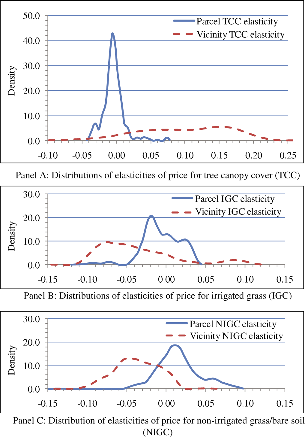
Let us now focus on the distributions of land cover variables (Figure 2). For tree canopy cover (TCC; Panel A), most parcel-level elasticities range between −0.04 and 0.02 (with p50 = −0.0047 vs −0.0106 for the SDM). By contrast, TCC vicinity elasticities tend to be larger and more spread out: they range mostly from −0.08 to 0.23 and p50 = 0.1045 is within one standard deviation of the SDM estimate of 0.1203.
GWRM distribution of elasticities of price.
By contrast, for irrigated grass cover (IGC; Panel B), parcel elasticities and vicinity elasticities overlap substantially. The former range from −0.05 to 0.05 and p50 = −0.0084 is within one standard deviation of the SDM median estimate. Vicinity elasticities are still more spread out and fall mostly in the interval (−0.12, 0.12) with p50 = −0.0480 vs −0.0094 for the SDM.
Finally, for parcel non-irrigated grass (NIGC; Panel C), parcel elasticities tend to be larger than vicinity elasticities, but their spread is closer: (-0.05, 0.10) (p50 = 0.0123) for the former versus (-0.10,0.02) with p50 = −0.0386 for the latter.
5.3 Robustness Checks
To assess further the robustness of our SDM results, we contrasted log–log and log–linear models using AIC and BIC; we found that the former outperformed the latter for both measures. We also performed a RESET test on our preferred log–log model and rejected the null hypothesis that power combinations of the estimated values help to explain the logarithm of the sales price of multifamily buildings (p-value = 0.349). In addition, we found that the three weight matrices we considered give very similar results. Except for vicinity TCC, the elasticities of price with respect to local land cover variables are small and not statistically significant. However, adding 1 per cent to TCC within 200 metres of a multifamily property would increase its value between a low of 0.0713 per cent (with a Delaunay matrix) and a high of 0.1203 per cent (with uniform weights and Zillow neighbourhoods; see Table 2).
Our sensitivity analysis for the GWRM focused on the value of the bandwidth used to weight nearby properties: we estimated models with bandwidths of 6–9 km. We found that the median values of the distributions of the land cover parameters (which are elasticities with respect to price here) are not sensitive to the value of the bandwidth, but the tails of these distributions are, especially for TCC and irrigated grass vicinity parameters. With larger bandwidths, the spread of the land cover elasticities shrinks as their left tails shift towards higher values, while their right tails shift to smaller values. Overall, these results suggest that most multifamily buildings in our sample would lose value with more trees or irrigated grass on their parcels, but their value would increase with more trees in their vicinity.
6. Policy Implications for Greening Los Angeles
As already mentioned, most multifamily building residents are renters. Although these renters may appreciate both trees and irrigated grass, our results show that property owners typically have no financial incentives to provide these amenities. By contrast, Saphores and Li (2011) found that more parcel irrigated grass and (to a much smaller extent) more parcel trees would increase the value of most single-family detached houses in Los Angeles. Several reasons may explain why multifamily building owners are not looking forward to increasing green spaces on their properties.
First, the maintenance costs of trees and irrigated grass areas can be substantial. Property owners could pass along some of these costs to their renters but they may instead try to keep costs down if their tenants are struggling economically.
Secondly, some of the benefits from green spaces (for example, air quality improvement or carbon sequestration) are public goods, so there are few incentives for a private party to provide them. Moreover, shade and the resulting energy savings, which are private goods, are likely to be insignificant for multifamily properties compared with single-family detached homes. Although adding more parcel trees to a property may benefit the owners of surrounding multifamily buildings, experience shows that private property owners are unlikely to negotiate compensations for those willing to take a loss to provide local public goods, probably due to high transaction costs.
Thirdly, landscaping may be competing with parking, which is essential in southern California’s auto-oriented development, so the opportunity costs of green spaces are likely to be substantial.
These results have implications for the tree-planting programmes that have sprouted up around the country and in Los Angeles in particular. Since September 2006, the city of Los Angeles has embarked on a major tree planting campaign (the Million Trees Los Angeles or MTLA), aiming to plant 1 million trees between 2006 and 2010 (McPherson et al., 2007), although that deadline was recently extended to 2013 or 2014. Given its ongoing budget woes, Los Angeles had planned to get private property owners to plant 70 per cent of MTLA trees—a much higher proportion than New York’s Million Trees programme (40 per cent), for example.
However, the pace of tree plantings has been much slower than expected: only 192 000 trees had been planted by the MTLA as of mid December 2010 (Burry, 2011) even though trees have been given for free to private landowners by five non-governmental organisations. This number excludes the 56 000 trees sold by Home Depot stores in Los Angeles between fall 2006 and the end of 2010 that were curiously included in the MTLA official tally. In addition, we should mention that small giveaway trees (41 000 of these 192 000 trees were seedlings and bare-root trees) typically experience much higher mortality rates than trees planted by specialists.
The modest success so far of the MTLA may seem surprising since McPherson et al. (2011) found that each new tree in Los Angeles will provide average annual benefits ranging between $38 and $56 depending on mortality scenarios. However, their study quantifies only benefits and ignores costs linked to tree planting and upkeep. Secondly, their estimated benefits are averaged over 35 years without discounting. Most importantly, over 80 per cent of their benefits are in the ‘aesthetic/other’ category and they were calculated from results obtained by Anderson and Cordell’s (1988) study in Athens, Georgia.
Hence, available space for planting new trees, which was highlighted in McPherson et al. (2007), should not be the main criterion for a large tree planting programme. In addition to accounting for the preferences of residents and landowners, it is important to consider who benefits from the expenditure of scarce public funds dedicated to tree planting. According to our GIS analyses, the average vicinity tree canopy cover for multifamily properties is approximately half of the vicinity TCC for single-family residences (19 993 square metres versus 30 714 square metres). Likewise, the average area of vicinity irrigated grass for multifamily properties is 12 815 square metres, compared with 17 731 square metres for single-family residences. Population density further exacerbates these differences. Although multifamily building residents are typically closer to public parks (0.8 km versus 1.0 km for single-family residents), the quality and the safety of these parks are often questionable. This situation should motivate efforts to explore the benefits and costs of neighbourhood green spaces, given mounting evidence of their health benefits (for example, see Takano et al., 2002).
7. Concluding Remarks
In this paper, we investigated the relationship between local land use and prices of multifamily properties sold in the city of Los Angeles in 2003 and 2004. We estimated a spatial Durbin model (SDM) and a geographically weighted regression model (GWRM) to deal with spatial dependence and omitted variable bias. A comparison between SDM and OLS results illustrated the perils of omitted variable bias, while our sensitivity analyses gave us confidence in the robustness of our findings.
Our analysis suggests that green spaces impact multifamily property values quite differently on parcels and in their vicinity. Our GWRM results suggest that increasing the parcel tree canopy cover of a multifamily building would typically decrease its value slightly, whereas increasing the tree canopy cover in its vicinity (200 metres outward from its parcel boundary) would enhance its value. By contrast, the impact of more irrigated grass is mixed. Our findings reflect that multifamily building owners have no financial incentive to provide more trees or irrigated grass areas on their property, even if their renters would enjoy them.
We therefore suggest that the city of Los Angeles explore the net benefits of planting trees on public land in the vicinity of multifamily buildings as there is growing evidence of links between urban green spaces, health and social safety (Groenewegen et al., 2006; Tzoulas et al., 2007). If public funds are spent on large tree planting programmes, equity considerations require focusing on the situation of disadvantaged groups.
Footnotes
Funding Statement
Financial support from NSF and EPA is gratefully acknowledged.