



Abstract
Based on a lifetime consideration, previous research has extended Frank’s graphical model with borrowing, property taxes and moving costs to analyse the welfare effects of housing appreciation and depreciation, and has shown that appreciation can make homeowners worse off, but homeowners’ welfare cannot decrease with depreciation. The latter is counter-intuitive, especially for owners with a high portion of mortgage in a housing slump. Alternatively, this paper treats property tax as an annual taxation and measures mortgage loan as a portion of house value when it was purchased. It is shown that if a house owner adjusts his/her house size in response to a price change, then with a low mortgage loan (or no mortgage), the owner will be better off only when there is a large appreciation or depreciation, while he/she cannot be better off under depreciation if he/she bought that house largely via a mortgage loan.
1. Introduction
In his microeconomics textbook, Frank (2006, pp. 166–167) shows that, starting from a fixed bundle of housing and a composite good, either an increase in the price of housing (appreciation) or a decrease in the price of housing (depreciation) makes an owner better off. 1 The intuition is as follows: a house owner can sell his/her house at a higher price after housing appreciation and use this revenue to purchase more composite goods with a constant price and thus raise his/her utility. On the other hand, after housing depreciation an owner can also sell his/her house and repurchase a larger house at a cheaper price. His/her utility is increased in the sense that he/she replaces the composite good with a cheaper good (housing). However, Frank’s (2006) model is too simple to capture some real-world factors such as property tax, mortgage loan and moving cost.
In a parallel study on this issue, Lai, McDonald and Merriman (2010) (LMM model, hereafter) 2 use a diagrammatic analysis 3 and a lifetime span consideration to verify the correction of Frank’s (2006) model with moving cost and mortgage loan. In the case of housing appreciation, their conclusion is close to that of Frank (2006). In other words, an owner will be better off if this appreciation is large enough to compensate for the fixed cost (moving cost or mortgage loan), while the owner will be worse off after a small appreciation. In the case of housing depreciation, the result is quite different. First, if there is no mortgage loan, the owner’s utility is definitely increased, no matter whether the owner moves to another house or not. This is because the property tax liabilities fall. Secondly, if an owner still has some remaining mortgage balance, he/she will be better off by moving to another house with the optimal size if the depreciation is large. Even if the depreciation is small, by choosing to stay in the same house, the owner cannot be worse off due to the fall of property taxes liabilities. Based on these two points, the owner can never be worse off after housing depreciation. Is this right for the LMM model in reality?
The world economy encountered a financial crisis in 2008, which was initially caused by the collapse of the housing bubble in the US and many financial institutions holding mortgage or mortgage-backed securities being driven to near-bankruptcy. From July to December 2008, housing prices fell 27 per cent and 2.3 million foreclosures occurred (Mankiw, 2010). It is obvious that many house owners felt worse off during this financial crisis. Even now, the housing market has not returned to its normal track.
The LMM model is restricted by the diagrammatic analysis and some assumptions should be modified. For example, the lifetime property tax assumption in the LMM model can simplify the mathematical process, but it may not fit reality. In the real world, the property tax is an annual tax and is proportional to the housing value, and thus the tax payment can change from year to year due to housing price changes. Therefore, the composite good consumption is also affected by the property tax change. A crucial difference between this paper and the LMM model is that the LMM model considers the property tax to be included based on a lifetime framework, while this paper defines the wealth coming from a house as the total money that the owner can receive when the house is sold, which does not include tax. It is obvious that tax is paid to the government and cannot be counted as the owner’s wealth. Consequently, only when the price change is larger than the tax payment will an owner’s utility be raised. 4
Moreover, in the LMM model, the remaining mortgage loan is assumed to be a constant, something like a constant moving cost, to accommodate to their analysis framework. However, in the real world, a mortgage loan is, in general, a proportion of the original housing value. In a housing slump, the actual housing value is evaluated at the current price, but the monthly repayment is still based on the original price. The owner therefore may have great difficulty changing to another house, because he/she needs to pay back the loan, but his/her house value is no longer as high. Based on the observation in the real world, this paper develops a mathematical model with more reasonable assumptions such that the property tax is counted on an annual basis and the mortgage loan is a portion of the original housing value. It will be shown that house owners with a high portion of mortgage will be worse off during a housing slump, instead of being better off as Frank (2006) and LMM (2010) claim.
The rest of the paper is organised as follows. Section 2 is the model; section 2.1 recapitulates Frank’s (2006) model; section 2.2 revises the model to add property taxes; section 2.3 is the general case which includes property taxes and mortgage loans; section 2.4 discusses the choice of staying in the same house; section 2.5 is an extension; and section 2.6 provides two numerical examples. Some concluding remarks are discussed in section 3.
2. The Model
Suppose there is a city where each resident should have one house in this city. In order to ease our analysis, a Cobb–Douglas utility function is employed hereafter as a standard example to depict the current model mathematically. Suppose each agent has a utility function
Solving for the Lagrangian
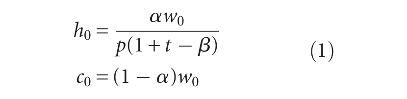
The equilibrium indirect utility is then
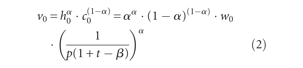
Suppose the housing price now changes to p′. The new wealth is then
This is because his/her current housing value is now p′h0, while his/her mortgage is still βph0. If the agent decides to change the house size, then he/she must first pay off the old mortgage loan and apply for a new mortgage loan. 7 The Lagrangian is thus

Solving for the Lagrangian yields

The indirect utility function is therefore
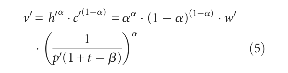
We should notice that the major difference between LMM’s assumptions and those in the current paper is the definition of wealth when housing prices change. Precisely speaking, in their model, the new wealth after housing prices change from p0 to p′ is
Note that the agent has another choice, which is staying in his/her current house. If he/she stays in the original house, it can be considered that he/she repurchases his/her house with the current conditions each year. 8 The new wealth in this case is

where, the subscript A represents the case where the owners stay in their original houses. The Lagrangian in this case is thus

where,

The indirect utility function is then

The purpose of our analysis is to compare the relative utility of a house owner before and after housing price change. Dividing equation (5) by equation (2) yields
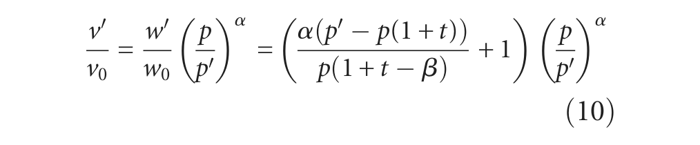
In order to ease our mathematical derivation, we define a new function g as

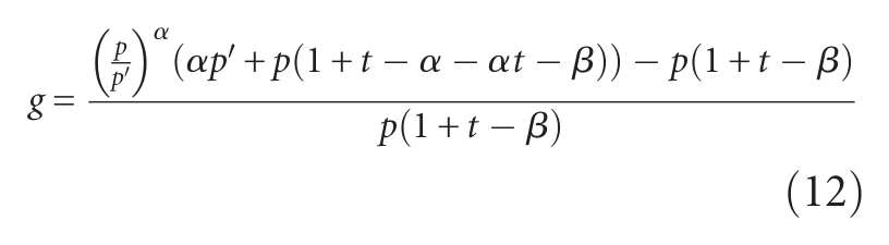
It is clear that the change in the price of housing makes a house owner better off if g > 0, in the sense that v′ > v0. Conversely, a house owner feels worse off after housing price change if g<0, in the sense that v′ < v0. Since the denominator in equation (12) is unambiguously positive, the sign of function g depends only on the numerator in equation (12). If the numerator in equation (12) is positive, then g > 0 and v′ > v0. If the numerator in equation (12) is negative, then g < 0 and v′ < v0. The following discussions will be separated into three parts.
2.1 When t = 0 and β = 0 (Frank’s case)
In Frank’s (2006) case, there are no property taxes (t = 0) and no mortgage loans (β = 0). Substituting t = 0 and β = 0 into equation (12) yields

Substituting p′ = p into equation (13) yields

Differentiating equation (13) with respect to p′ yields

It is clear that

It follows that the function gF is concave in p′ if
Proposition 1. When t = 0 and β = 0, then v′ > v0 if p′ ≠ p and v′ = v0 if p′ = p. In other words, Frank’s (2006) result is correct when there are no taxes and no mortgage loans. A new finding is that gF is concave (convex) when
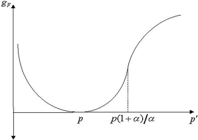
The function g when t = 0 and β = 0 (gF).
2.2 When t > 0 and β = 0
When a property tax is introduced and house owners do not use any mortgage loans, then substituting β = 0 into equation (12) yields

Differentiating equation (15) with respect to p′ yields
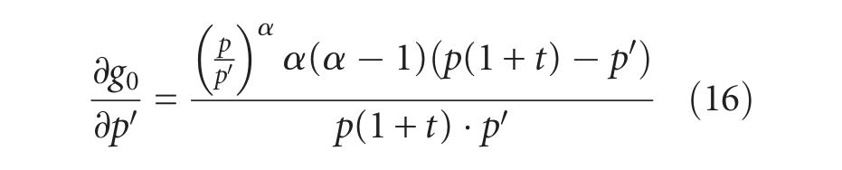
From equation (16), the sign of

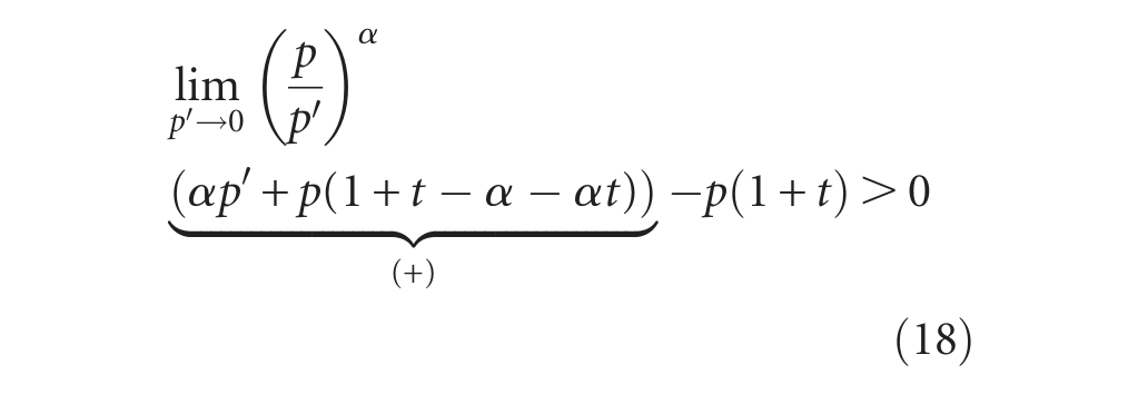
Similarly, the sign of function g0 depends only on the numerator in equation (15). The following equation (18) indicates that the value of the function g0 is positive when p′ is approaching zero. 9
The second-order derivative of the function g0 is calculated as
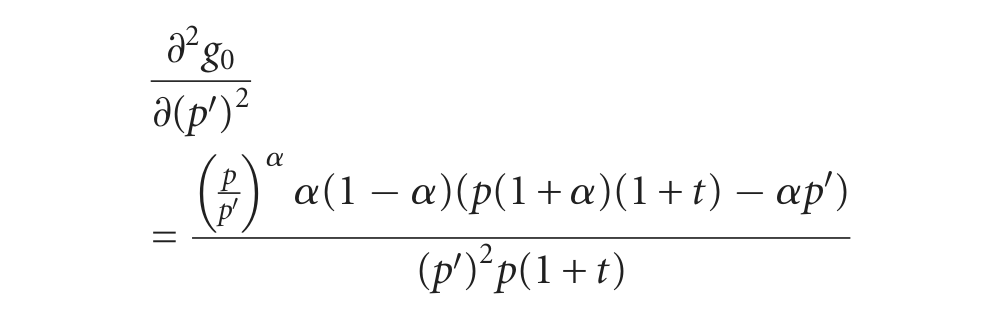
It follows that the function g0 is concave in p′ if
Combining equations (16), (17) and (18), the function g0 can be depicted as Figure 2. Note that g0 > 0 if
Proposition 2. When t > 0 and β = 0, then v′ > v0 if
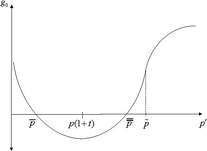
The function g when t >0 and β = 0 (g0).
The implication of Proposition 2 is that, when there is no mortgage, v′ (the utility of changing to the house with an optimal size) is higher than v0 (the original utility level) when housing price appreciation (depreciation) is large. If this price change is not sufficiently large, then changing to a new house (with optimal size) makes the owner worse off, because the benefit of appreciation (depreciation) is less than the property tax payment. 10
2.3 When t > 0 and β >0 (the general case)
The general case 11 of our model is more complicated. To reach this general case, several steps will be employed. First, the first-order derivative of function g with respect to p′ is calculated as
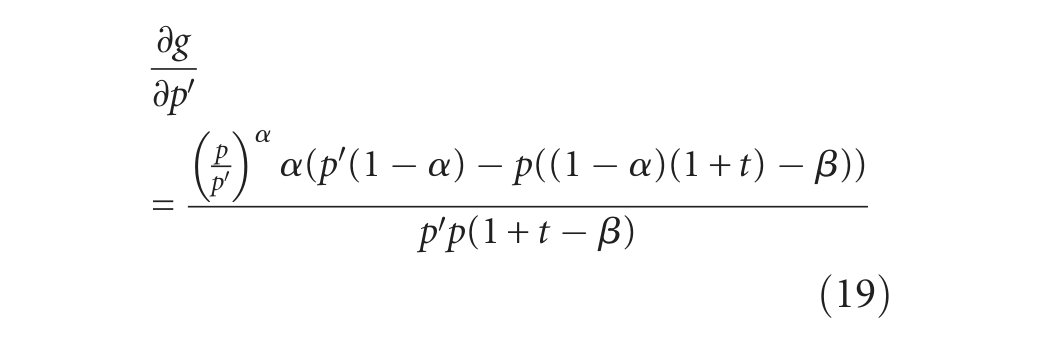
Solving

Note that p′a is the critical value of p′. From equation (19), the sign of
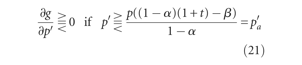
Secondly, we check the sign of function g when p′ is evaluated at the critical value (i.e. the stationary value of function g). Subtracting p from p′a yields

Substituting p′ = p into equation (12) yields
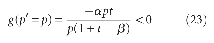
If the numerator of equation (22) is positive, then p′a > p. In this case,
Finally, we then check the sign of function g when p′ approaches zero.

The sign of equation (24) depends on the numerator of equation (24). If
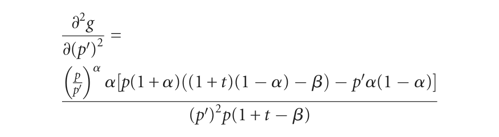
It follows that the function g is concave in p′ if
Proposition 3. Suppose t > 0 and β > 0. When
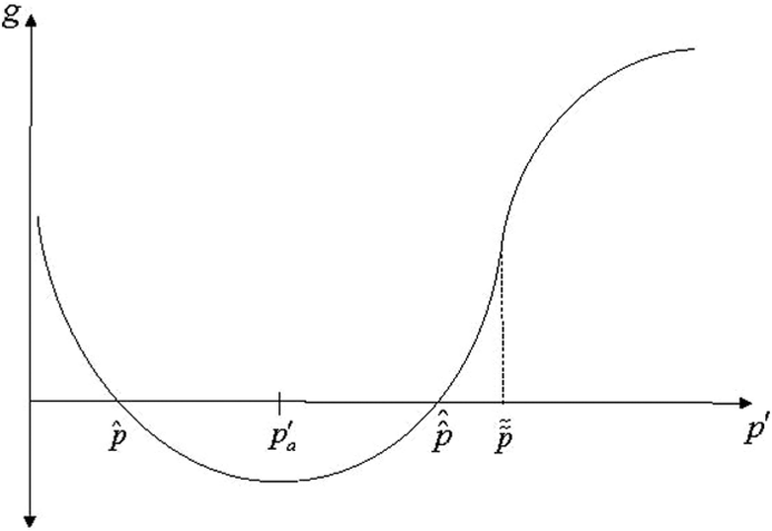
The function g when t > 0 β > 0, and

The function g when t > 0, β > 0 and
The intuition of Proposition 3 is as follows. For a housing price change, a house owner can sell his/her house at a higher price after housing appreciation and use this revenue to purchase more composite goods to raise his/her utility. In contrast, an owner can also sell his/her house in a depreciation case and repurchase a larger house with a cheaper price and raise his/her utility. However, if a property tax is considered, an owner is better off only when the appreciation or depreciation is large enough to compensate for the tax payment. Furthermore, if a house is financed through a mortgage loan, two situations should be clarified. In a housing appreciation, an owner is obviously better off, because the housing value is increased, while the mortgage loan remains constant (based on the original price). In a housing depreciation, an owner is unambiguously worse off, because the housing value is decreased, while the mortgage loan remains constant (based on the original price). Therefore, when the percentage of a mortgage loan over the total housing price is relatively low (
2.4 The Choice of Staying in the Same House
A house owner always has the option of staying in the original house when the housing price changes. The utility of this situation is denoted by vA in equation (9). There should be no difference between the analysis of changing to a new house and the analysis of staying in the same house except that an agent needs to incur a moving cost if he/she chooses to move.
If a fixed moving cost is incorporated into the model, the previous conclusions in the paper are basically held, and those equations are omitted here to save space. The conclusions of the general model with moving cost are as follows. 12 First, if the percentage of a mortgage loan over the total housing price is relatively low, then the owner is better off (worse off) under a large (small) appreciation or depreciation. Furthermore, an owner changes to a new house only if the housing price appreciation or depreciation is large enough. Secondly, if people buy their houses largely relying on a mortgage loan, it is impossible for them to be better off when the housing price falls. An owner stays in the same house under small depreciation, but changes to a new house under large depreciation. Our results can be used to explain the observation that some people who had bought their houses with a high portion of mortgage felt worse off under a housing market slump during the financial crisis in 2008, instead of being better off as predicted in Frank (2006) and LMM (2010) models.
2.5 Extension
In the housing depreciation case, the owners may have another choice, which is very common in reality. That is, he/she can hand over the key to the bank and move to another house. 13 In this case, the critical point for handing over the key to the bank is p′ = βp. In other words, when p′ < βp, the current value of his/her house is p′h0, which is less than his/her mortgage loan βph0. Therefore, if he/she chooses to return the house, his/her new wealth is c0 instead of w′. The Lagrangian is thus

where the subscript K represents the case of handing over the keys to the bank. Solving for the Lagrangian yields
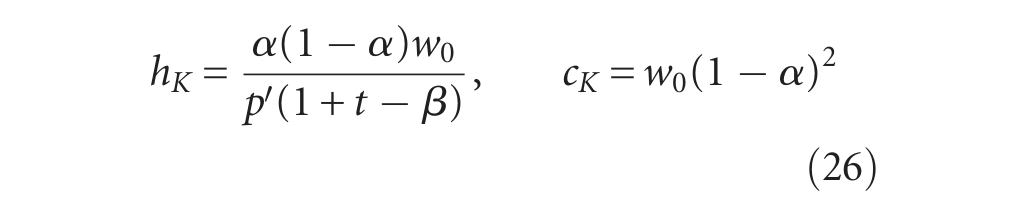
The indirect utility function is therefore

Comparing equations (25) and (3), we find that the two optimisation problems are the same, except that w′ is replaced by a larger c0 when p′ < βp. It is unambiguous that
However, in the real world, when a house owner hands over the key to the bank, he/she may not be able to get another mortgage from the bank. Therefore, β = 0 in equation (25) and the critical point of handing over the key is less than βp, which is the critical point when β > 0 . In the next section, we will use numerical examples to demonstrate how the owner decides whether to hand over the key or pay back the mortgage and move to another house.
2.6 Numerical Examples
Two numerical examples (low mortgage loan, high mortgage loan) will be demonstrated in this section. First, suppose that w0 = 100, t = 0.02, α = 0.3, 14 β = 0.3, z = 2 and p = 10. 15 This is shown as a general case with a low mortgage loan. As seen in Figure 5, v′ is greater than v0 whenever p′ < 2.484 or p′ > 12.080. Note that vA is greater than v′ when the change in housing price is small (5.490 < p′ < 15.975) and that owners are better off either under large appreciation or large depreciation. Moreover, consider the appreciation case; note that when housing appreciation is very small (10 < p′ < 10.714), an owner will stay in the same house and his/her utility is lower than v0. When appreciation is larger (10.714 < p′ < 15.975), the owner will choose to stay in the same house and his/her utility is higher than v0. When appreciation is even larger (p′ > 15.975), the owner will move to another house with an optimal size and his/her utility is higher than v0. Consider the depreciation case: with a small depreciation (5.490 < p′ < 10), an owner will stay in the same house and his/her utility is lower than v0. When depreciation is larger (2.484 < p′ < 5.490), the owner will change to another house and his/her utility is still lower than v0; and when depreciation is even larger (p′ < 2.484), the owner will move to another house with an optimal size and his/her utility is higher than v0.
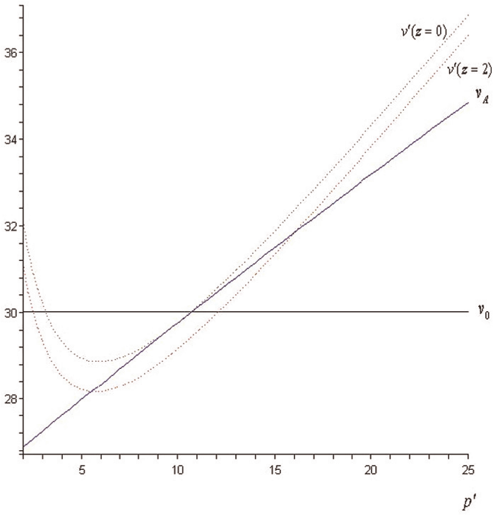
The general case when β is low.
Secondly, if t = 0.02, and w0 = 100, α = 0.3, β = 0.85, z = 2 and p = 10, then v0, v′ and vA can be drawn as in Figure 6. Note that the v′ curve intersects the v0 curve once (p′ = 10.377), meaning that if the house owner changes to a new house with optimal size, only the appreciation case can make the owner better off, while the depreciation case never enables the owner to be better off. Moreover, vA is greater than v′ when the change in housing price is small (when 7.408 < p′ < 15.868). This means that with a large appreciation or depreciation, the owner is worse off staying in the same house than moving to a new house with optimal size. Finally, we also draw two lines
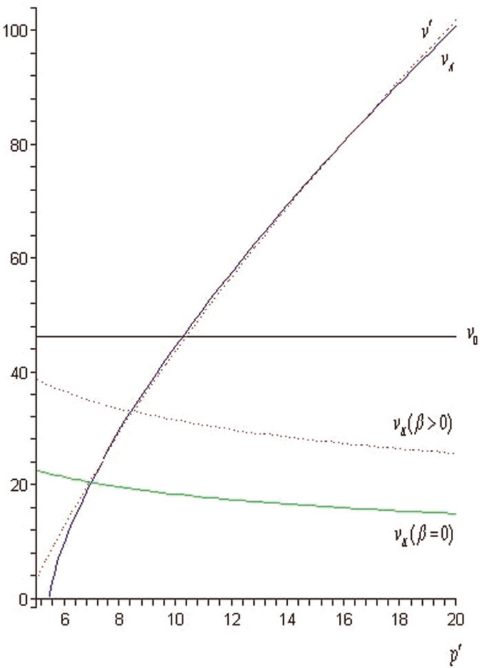
The general case when β is high.
3. Concluding remarks
Frank (2006) provides a paradoxical example which demonstrates that housing appreciation and depreciation can both benefit owners. The LMM (2010) model embodies factors (borrowing, property taxation and moving costs) into Frank’s (2006) model from a lifetime span and shows that appreciation can make house owners worse off, but can never make them worse off under depreciation if the house owner chooses to stay in the same house. The current paper constructs a general model similar to the LMM model, but under an annual basis, stressing that a person needs to pay an annual property tax, and the mortgage loan is a percentage of the house value. Thus, it is shown that Frank’s conclusion is valid only for those cases with no property tax, no mortgage loans and no moving costs. A new finding on Frank’s (2006) model is that the function of utility difference is first convex and then concave in the appreciation case. With a property tax, a small change in the housing price never raises the owners’ utility. When people buy their houses largely relying on a mortgage loan, it is impossible to be better off when the housing price falls, which is very different from the conclusions recommended in the LMM model.
Specifically, housing appreciation is not always better for owners who intend to adjust their house sizes when a property tax is considered, especially for a small appreciation. If the gain coming from appreciation does not cover the property tax payment, then the owner is still worse off. For the depreciation case, changing to a new house may not be the best choice for owners when property tax and moving costs are considered. More importantly, if people buy their houses largely relying on a mortgage loan it is impossible for them to be better off when the housing price falls, no matter whether they stay in the same house or not. This result is close to the reality during the financial crisis of 2008, especially for house owners financed by sub-prime and related loans. When a housing market slumps, people who bought their houses with a high mortgage loan will be worse off, instead of being better off as predicted in the Frank (2006) and LMM (2010) models. This is because an owner cannot pay off his/her mortgage loan due to the house value no longer being so high.
Since our model is fully analytical in mathematics, our model can be a benchmark and could be extended to other related issues for future study. It is worth delving deeper into policy implications. For instance, in the US, starting from the mid 1990s, but accelerating after 2000, the east and west coasts and some metropolitan areas inland have experienced housing bubbles (see Schwartz, 2010, for details). A government may enact a mortgage restriction on the total outstanding loan or a ceiling of the loan-to-value ratio in order to prevent overbanking and the consequent housing bubbles, especially for low-income people, because some of them may be forced to hand over their houses to the bank and encounter some difficulties in a housing slump.
Moreover, housing is one kind of long-run asset, instead of a short-run speculative asset. A government may enact a variable property tax rate to dampen the extraordinary fluctuation of housing prices. Therefore, an optimal property tax scheme based on long-run considerations is also a possible future research direction. Finally, since our analysis is based on the demand side, a proper policy evaluation should also consider the supply side of a housing market, therefore the social welfare implications of a property tax or housing subsidy on the efficiency of the housing market could also motivate further study.
Footnotes
Funding
This research received no specific grant from any funding agency in the public, commercial or not-for-profit sectors.