
Abstract
The concept of an urban growth wave expanding outwards is used to examine the commuting characteristics of residents of recently developed housing areas within the 50 largest US metropolitan areas at multiple points of time between 1980 and 2000. The results show that not only do areas of recent housing booms have longer commuting times and differing socioeconomic characteristics than older parts of the cities, but this commuting time will subside as these areas age (although average commuting times may rise for the entire metropolitan area). Like a growth wave, a commuting transition move outwards and therefore newer growth areas (or sprawl) should be considered as a temporary stage in the ongoing process of urban growth. Focusing on building cycles avoids the pejorative sprawl label and reconceptualises this sort of low density, auto-dependent urban form as a normal part of the urban growth process.
Introduction
Within American cities, the areas where urban land transitions into rural land has been considered problematic for at least 80 years, in part because it lies outside the traditional interests of rural and urban geographers and due to the difficulty of conceptualising this area (Wehrwein, 1942). It was realised that cities cannot be accurately represented by the static zones of von Thunen’s isolated state or the concentric ring model of urban structure, and neither would the built-up area be correctly represented by city limits. Discussions of ‘exploding cities’ in the US in the 1950s created an approach to urban growth based on the metaphor of a wave sweeping outwards into the countryside (Blumenfeld, 1954). In recent decades, interest in the urban periphery has again become significant but researchers have returned to the mapping of static land use and density patterns, now termed sprawl. This topic has received tremendous attention from the media as well as scholars (Bengston et al., 2005) and is the focus of considerable debate. Some scholars perceive as it as a new phenomenon in urban development processes in the US, although others argue that sprawling growth patterns have always been visible in most prosperous cities in the US, as well as everywhere in the world where there is a certain measure of affluence and where citizens have some choice in how they live (Bruegmann, 2005).
Considerable efforts have been devoted to defining and quantifying urban sprawl so that this urban development and its associated negative consequences, such as more travel, greater reliance on cars, absence of public transport, additional use of energy, increased costs in providing utilities and the loss of open space, can be better understood (Burchell et al., 1998; Sultana and Weber, 2007). However, there has been little consistency as to exactly what this phenomenon is and how it can be defined. Sprawl is often treated as a static pattern, measurable by low population or housing densities (Malpezzi, 1999; El Nasser and Overberg, 2001; Galster et al., 2001; Ewing et al., 2003; Hasse and Lathrop, 2003; Lopez and Hynes, 2003; Wolman et al. 2005), although some also incorporate other dimensions of urban form, such as compactness, land use patterns or the configuration of street networks (Galster et al., 2001; Ewing et al., 2003; Tsai, 2005; Wolman et al., 2005).
Yet American urban areas are dynamic places—areas that might have been considered sprawl a few decades ago are now quite dense and urban (Bruegmann, 2005) and areas currently regarded as sprawling may likewise be seen as fully urban in the future. Seen from this point of view, one can consider recently built low density housing areas of cities (or sprawl) as a temporary stage in the on-going process of urban growth and development. While some approaches to sprawl have considered rapid population growth, none of the recent work on sprawl has examined the way in which it is transformed into more dense urban areas over time.
One way of doing this is to use the metaphor of urban growth as a wave to describe urban expansion as a dramatic transition in land use on the edges of metropolitan areas. We incorporate this notion to examine the commuting characteristics of residents of recently developed areas at multiple points of time in order to investigate how commuting is related to this growth process. We expect that areas built at a particular time will have a distinct commuting pattern (length, mode choice, etc.), which gradually changes as an area matures. This process should create a commuting transition of rapid increases in commuting time followed by gradual decreases. The results of this study show that in fact not only do areas of recent housing growth in American cities have longer commuting times than other parts of the city; but this commuting time will go through a predictable commuting transition as these areas age.
Theoretical and Conceptual Background
Urban Growth and Housing Cycles
The growth of cities and their expansion into surrounding rural land have been studied from many perspectives, including the conversion of agricultural land to urban land (Greene, 1997; Theobald, 2001), as a metropolitan bow wave (Hart, 1991) or using the metaphor of an urban growth wave (Blumenfeld, 1954; Gober and Burns, 2002). Adams (1970) discussed the growth pattern of US cities in terms of the building cycle, as cities do not grow evenly but in discrete housing booms in which large amounts of housing and other buildings are built, followed by a slowing down of construction activity for several years. He discussed these booms in the context of transport technology and showed that construction booms between 1890 and 1960 took place in particular transport eras. In addition to new housing being located farther out from downtown, different housing and neighbourhood forms emerging, and changing demographics or architectural styles, each housing boom was based on the availability of different transport systems. Characteristics of housing design, lot types and street patterns can be identified for different periods, although many neighbourhoods will contain a range of features (Moudon, 1992).
The first boom he discussed (peaking in 1905) took place during the heyday of the electric streetcar era and reflected this technology. Early streetcar communities were built with narrow lots on a grid pattern and values decreased away from streetcar lines. The next booms (peaking in 1925 and 1941) took place in the early auto era, at a time when streetcar lines were declining in prominence. House lots were wider to allow for driveways and garages, and building densities were much lower. New residential areas were built at considerably farther distances from the city centre than were previously possible. Two post-war booms took place at a time when the automobile had little or no competition as a commuting mode and when freeway systems were rapidly transforming cities. This of course is the beginning of the stereotypical automobile-oriented suburban period. Wider lots on various types of curvilinear networks became more common. These different neighbourhood and network forms each have densities which may have either decreased (common for single-family homes) or increased (for apartment complexes) over time. Hybrid patterns may come about because of redevelopment of older communities.
According to Adams Each successive growth ring captured the flavor of the living styles, income levels, transport technologies, spending habits, and tastes of its period. The landscape increment of each growth era remained remarkably stable in structure and layout during successive growth periods. The only exception to the persistence of prior arrangements was the slow yet steady migration of the shopping core of the central business district towards the most fashionable high income sector of the city (Adams, 1970, p. 51).
This retail migration has of course continued, leaving most large cities without any significant retail downtown. While housing in an area developed during a boom may remain largely unchanged, arterial roads near these areas can be expected to undergo a continuing process of redevelopment. Early commercial properties may appear early on, to be replaced as larger and more intensive developments arrive. This can obviously be expected to have an impact on commuting patterns (and even more so on shopping or entertainment trips).
The Building Cycle and Commuting
One of the most direct and observable ways building cycles can alter urban form and growth and transport patterns is by changing density. Newman and Kenworthy (1989) claimed that denser cities offered a number of advantages for commuting. In turn, Gordon et al. (1989) and Gordon et al. (1991) argued that commuting times were higher in dense cities and actually fell in rapidly growing cities. This ‘commuting paradox’ was explained by the likelihood that households and/or firms were rationally relocating to reduce commuting times (Levinson and Kumar, 1994; Sultana, 2000).
The associations between low densities and longer commutes have been examined at the neighbourhood level (for example, Handy, 1996; Malpezzi, 1999; Ewing and Cervero, 2001). At this scale low densities reduce the presence of work opportunities in the local environment, producing longer commutes. However, Ewing et al. (2003) examined density effects on congestion and commuting time and found no statistically significant relationship between residential density and commuting time, although a denser and finer street layout was associated with increased congestion and higher commuting time. More recent commuting research has examined fast-growing areas with low density development (sprawl) and their commuting characteristics. Sultana and Chaney (2003) confirmed that commuting times are highest in areas with low density and recent rapid growth, while Sarzynski et al. (2006) found that faster-growing cities have longer commute times. However, Sultana and Weber (2007) found that low density and fast-growing areas are associated with longer commutes, whether measured by time or miles. The relationship between population density and mode of transport has been well studied and confirms that areas with lower population density have fewer journeys by public transport while higher population density has a significant positive relationship with use of public transport and significant negative relationship with automobile use (for example, Steiner, 1994; Cervero and Gorham, 1995; Levinson and Kumar, 1997; Filion et al., 2006).
Given that explanations for population density and commuting often emphasise job opportunities, it is appropriate that employment density and commuting have also been examined. Some have found that not only may higher density employment be associated with higher commuting times (Gordon et al., 1989; Malpezzi, 1999), but in other cases low density workplace locations are associated with lower commute times (Sultana, 2000; Crane and Chatman, 2003) or had no relation to commuting at all (Gordon et al., 2004). Sarzynski et al. (2006) defined density by combining both housing units and the number of jobs on developable land and found a statistically significant positive relationship between densities and commute time. Low density and rapidly growing employment patterns outside urbanised areas have also been examined (Weber and Sultana, 2008). This analysis found that workers who commute to jobs in these areas travel shorter distances, often spend less time commuting, are less likely to drive alone and are more likely to bike and walk, although they do not earn as much as workers in urban areas. This suggests that low density job locations could actually improve commuting conditions in two ways: workers may relocate to find jobs nearby; and less dense areas may have lesser rates of daily traffic per freeway lane with correspondingly reduced average hours of delay. Employment decentralisation can therefore be expected to contribute to reducing commuting time by allowing for greater opportunities for rational relocation.
The Commuting Transition
Using the idea of residential growth as a wave pushing outwards and the importance of density to travel, commuting patterns within the city should also show a wave pattern. As the city develops outwards during a building cycle, newly built areas will experience an increase in commuting times because they are far from employment and have low density. Eventually commercial growth will occur, further increasing building densities (giving a more urban feel) and offering reduced commutes. The housing booms Adams discusses are also therefore commuting transitions between rural to urban commuting patterns (with a rapid increase followed by eventual decrease in commuting times). This can be seen in Figure 1, where successive time-periods show the area of peak commuting moving outwards. Since average commuting times increased nationally from 22.4 to 24.3 minutes between 1990 and 2000, a long-term increase in commuting times is also included. The hypothesis of the commuting transition was evident in Millward and Spinney’s (2011) work where they found that average commute time increased progressively outwards along an urban–rural gradient in a small city at one point in time.

Hypothetical commuting transition with increase in average commuting time.
Since Adams (1970) examined nation-wide construction up to the late 1960s, several housing booms have taken place. One boom peaked in 1973 before reaching a trough in 1976, and a lesser boom took place in the late 1970s, peaking in 1979 before bottoming out in 1982. This trough was short lived, as a third boom peaked in 1983 before declining to 1991. Homeownership actually declined during this period. Since that year, housing construction (and homeownership) continued to increase throughout the 1990s before rapidly increasing in 2004 and peaking in 2006. These booms provide a means of testing whether commuting patterns are related to building cycles in the form of a commuting transition.
Data, Unit of Analysis and Methodology
This study uses 1980, 1990 and 2000 US census data for a set of metropolitan areas to find evidence of the commuting transition within the outward growth of cities. In this research recent urban growth refers to housing constructed during recent housing construction booms in each census. To identify these areas, fine resolution data within metropolitan areas are essential. This study therefore uses block groups as the level of analysis, as these are the smallest zones for which both housing and commuting data are available. While the US Census Transportation Planning Package and National Household Transportation Survey contain far more detailed commuting data, they do not contain information on housing construction. Detailed sources of housing data and urban change exist, such as parcel data, the National Land Cover Data (NLCD) and residential building permit data, but these provide no information about commuting patterns (Fagan et al., 2001; Carlson and Dierwechter, 2007).
Following Adams (1970), we use the median year of housing construction to determine the date at which the majority of housing in a census block group was developed. Each block group is then assigned to a decade representing a particular housing boom. If the date is before 1950, it is classified as older urban areas. For example, all block groups with a median year built date between 1970 and 1979 will be assigned to the 1970s housing boom. Because of new housing construction within previously developed areas, many block groups will be reclassified as being in newer housing booms during a later census. The 1970s housing boom will be the newest shown in the 1980 census and will represent recently built areas for that time. For the 1990 census, the housing boom peaking in 1983 will represent recently built areas, while the 1970s areas will have become more established. For the 2000 census, the 1990s boom will be apparent, while those areas built during the 1970s and 1980s booms will have matured. Block groups outside the urbanised area boundary of a metropolitan area are classified as rural. Rural is therefore a residual category, which can be expected to include a diverse population (Dueker et al., 1983). These areas have not yet been incorporated into the urban fabric, although some may possess relatively recent housing.
Boundaries for Metropolitan Statistical Areas (MSAs) and Consolidated Metropolitan Statistical Areas (CMSAs, or groupings of MSAs) for 2000 were used, which provide continuity with earlier definitions going back to the 1950 census (Wyly et al., 2008). A total of 113 metropolitan areas had sufficient housing growth to have at least five block groups in each time-period for each of the three census years and the 50 largest of these were used in the analysis.
All of the commuting and housing data come from census SF3 files, based on the long form of the census questionnaire. Data for 2000 were obtained from the Census bureau website, while 1980 and 1990 data came from datasets created by GeoLytics Inc, 1 which allowed both 1980 and 1990 data to be extracted using 2000 block group boundaries. The 1980 census was the first to report commuting time and so is the farthest back the study can examine. However, commute time data are self-reported in the census, which may therefore be imprecisely reported due to rounding or recall error (Wachs et al., 1994). They also have not consistently been reported separately by mode in census data and hence aggregate travel times may be longer in areas with well established public transport systems because travel speeds on public transport are generally slower than for autos (Sarzynski et al., 2006). Aggregate commuting time was divided by the number of workers who work outside the home to create mean commuting time. Mode choice variables were also constructed, as was the percentage working in the central city of the MSA. These numbers are taken to be indicative of commuting patterns of the boom developed over the previous decade.
The SF3 data allow the calculation of the average number of rooms, percentage of homes with more than four bedrooms, average home value, average household income, average cars available, percentage of housing units occupied by owners, population density, household density and housing density. The percentage of homes built in the previous 10 years was calculated, as was the percentage of households moving into their current homes in the previous 10 years. Socioeconomic variables, such as the percentage of the population that is White, African American, Asian and Hispanic, were calculated, as was the percentage of households with children present.
Results and Analysis
Figure A1 in the Appendix shows the actual commuting transition patterns for the 50 largest metropolitan areas. The majority of cities show highest average commuting times within newly developed areas. Commuting times rise as an area is developed, then fall as these areas age. Cities such as Los Angeles, Phoenix and New Orleans show the pattern very clearly. Midwestern cities often show the highest commuting times in rural areas, reflecting the large rural population in these states. Chicago is an exception and appears more like cities on the west and east coasts. South-eastern cities show a more pronounced transition and also often show higher rural times, except for Atlanta and south Florida. Western, south Florida and northeastern cities have a strong transition, although often with lower rural times.
Table 1 shows mean travel time for newly built and older areas in the 1980, 1990 and 2000 censuses for the 50 largest MSAs. The hypothesis of the commuting transition leads to the expectation that 2000 commuting times will be significantly greater in areas built in the 1990s than in areas built in each of the previous booms. Similar patterns should be apparent for the 1990 and 1980 censuses. Analysis of variance (ANOVA) a priori contrast tests were carried out to determine whether significant differences in commuting time exist between recently built areas and all previously built areas in a city. This confirms the pattern seen in Figure A1, as a priori contrast tests show that in 2000 the majority of cities (41 of 50) have significantly different commuting times between newly built housing and all other previously built areas, and in each case recently built areas had higher commuting times. For 1990, all but four cities had significantly different commuting times, as did every city in 1980, with newly built areas having significantly higher travel times except in three cases. In each year, larger cities are clearly more likely to show significant differences and fit the commuting transition pattern better. Only nine of the 50 largest metro areas in 2000 did not show significant differences between newly built and previously built areas.
Mean travel times

Notes:
Commuting times of recently built areas were also contrasted with those of each previous housing boom with the ANOVA post hoc contrast Scheffe test. This test compares each group against the others to find out which group differs from the others (Rogerson, 2010). In this case, newly built areas were treated as a contrast and tested against each of the older periods. In only two cities were commuting times in older areas both significantly different and greater than commuting times in recently built areas. Larger cities are again clearly more likely to show significant differences between newly built areas and others.
If urban growth is taking place in a manner similar to Adams’ growth waves, then the high commuting times of newly built areas should be clustered in contiguous areas. Spatial autocorrelation tests using the Moran’s I measure were therefore carried out using GeoDa software (Anselin et al., 2006). This shows whether block groups with longer average commutes are adjacent to block groups with longer average commutes, and shorter commutes next to shorter commutes. Commuting times were indeed significantly clustered in every city for each year. The degree of clustering has decreased since 1980 for all but four cities, but did increase for 18 cities between 1990 and 2000 (in every case, the results were significant at the p = 0.05 level). The spatial growth of the majority of cities appears to have spread recent growth over a larger number of block groups, leading to a lessened concentration of high commuting times.
The Commuting Transition and Neighbourhood Change
A range of housing, household and commuting statistics was examined for four selected cities: Minneapolis, Portland, Atlanta and Phoenix (Table 2 and Figures 2–5). These four cities were selected to provide regional contrasts and connections to the larger literature on building cycles, urban growth and commuting. Phoenix represents a fast-growing city in the dry sunbelt, where urban growth has been limited by the availability of centralised water supply systems, while Atlanta represents the wet sunbelt, where urban growth is not constrained by infrastructural limits and sprawl is much greater (Lang, 2003). Portland is well known for its urban growth boundary and efforts to increase urban density (Weber, 2003), while Minneapolis represents Midwestern cities and was the site of Adams’ work on urban growth waves.
Detailed statistics for Minneapolis, Portlan, Atlanta and Phoenix

Notes:

Commuting, housing, and social characteristics by housing boom: Phoenix.
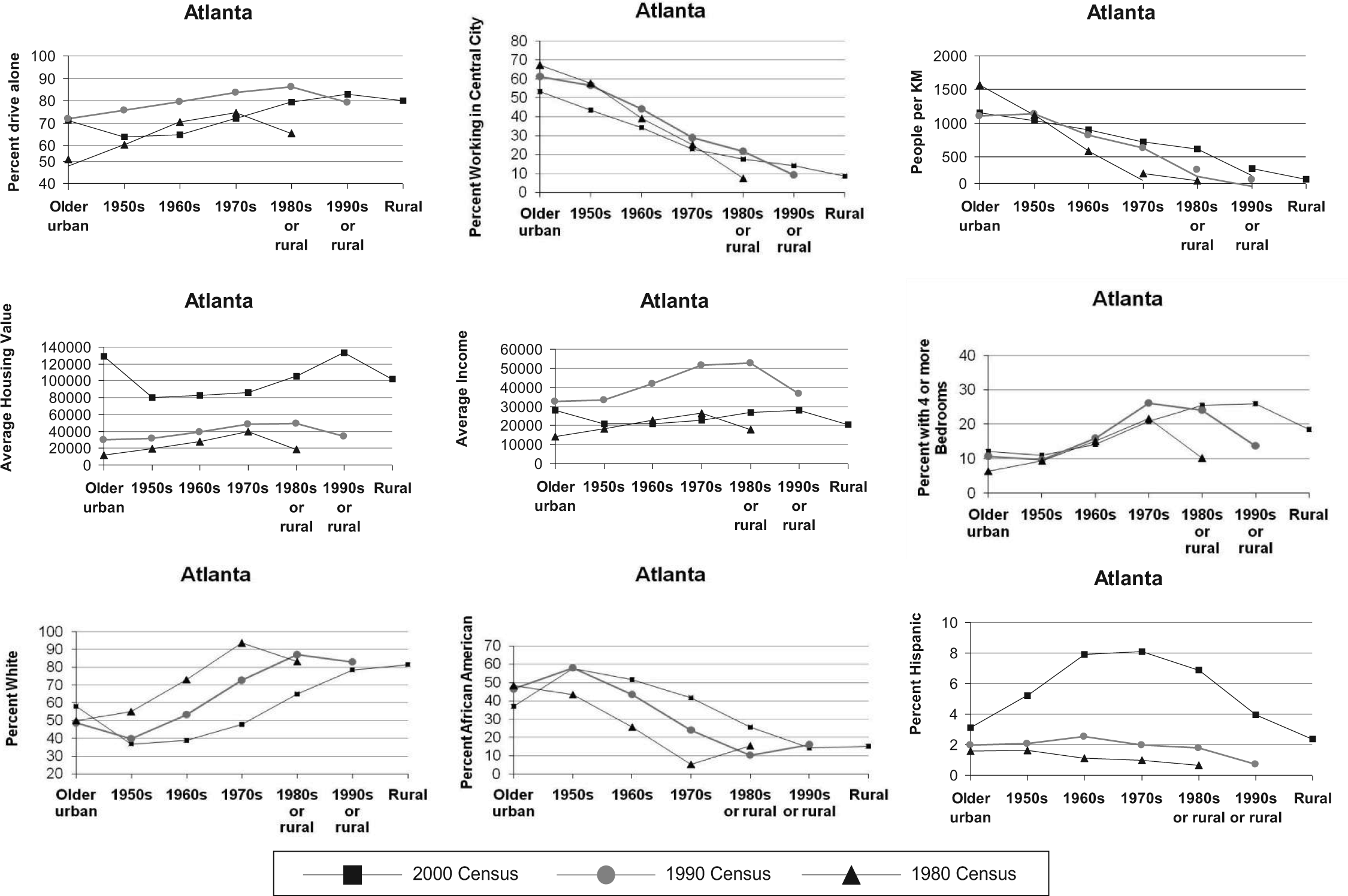
Commuting, housing, and social characteristics by housing boom: Atlanta.
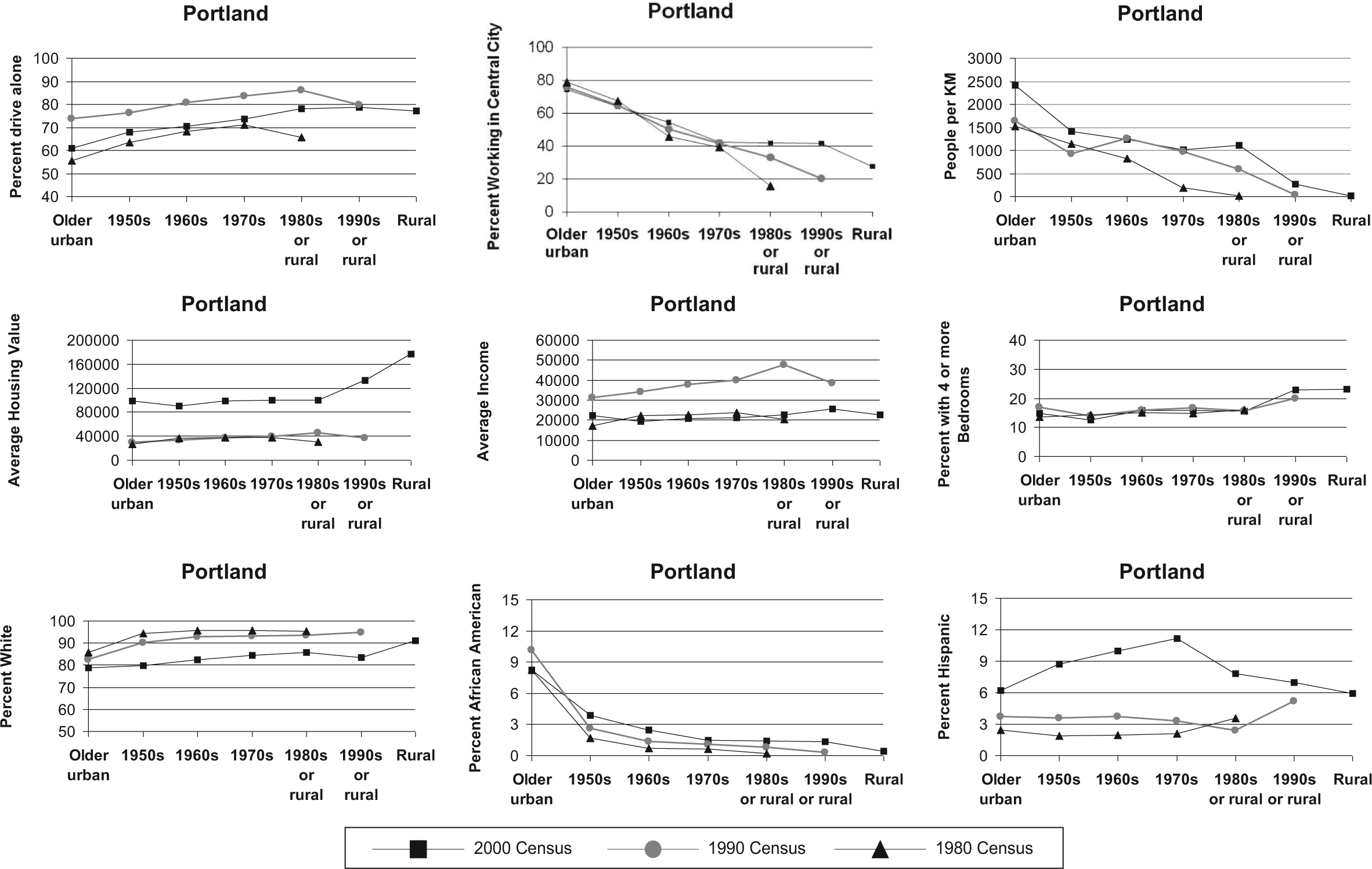
Commuting, housing, and social characteristics by housing boom: Portland.
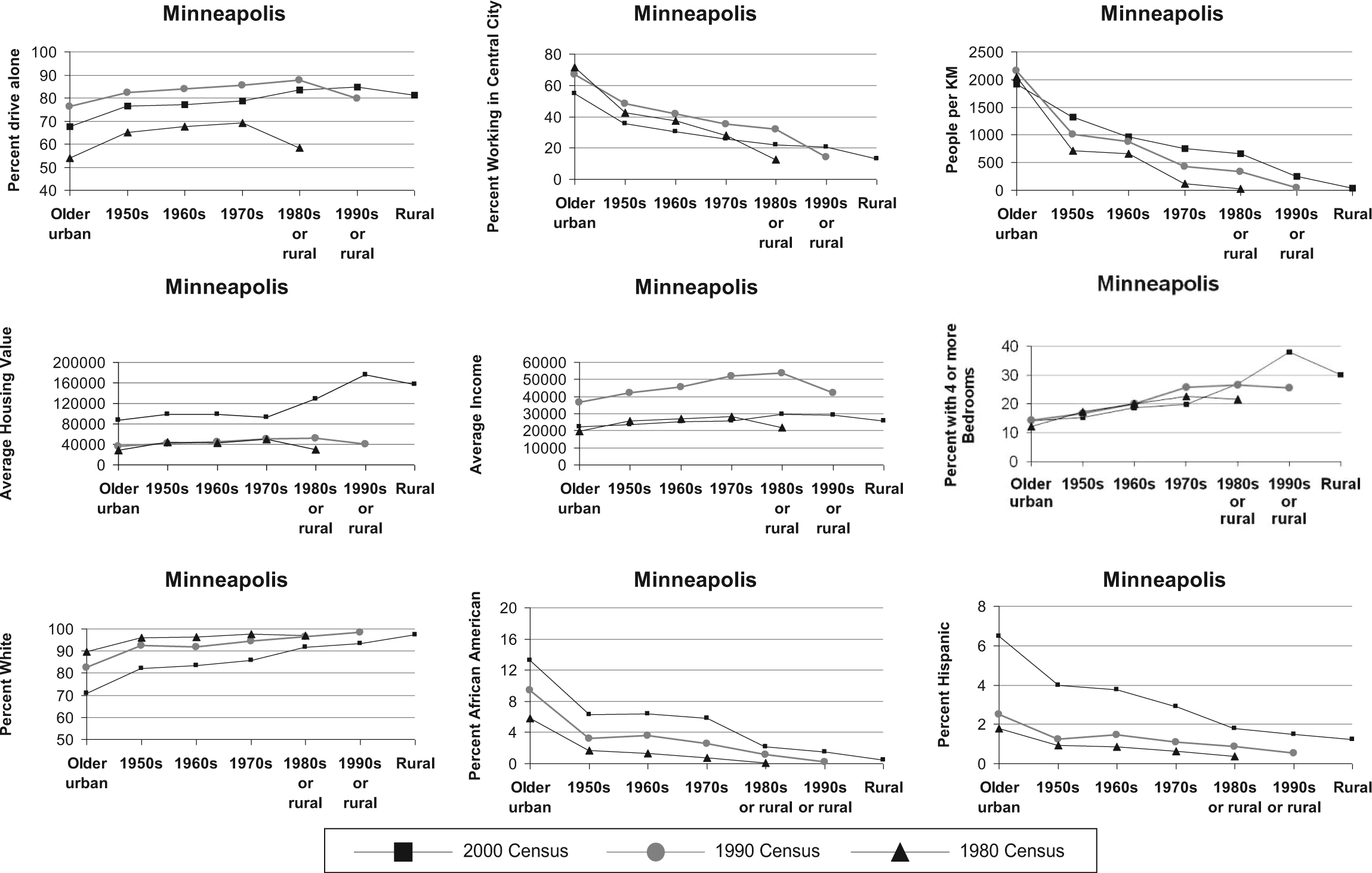
Commuting, housing, and social characteristics by housing boom: Minneapolis.
The ANOVA post hoc contrasts Scheffe test confirms that most characteristics in these four MSAs show the same pattern as for commuting time, with significantly different and higher values in newly built areas than that of each previous housing boom period. In many of the cases where the variables are not significantly different between boom periods, their magnitudes are everywhere low (as is often the case with the percentage walking or bicycling to work, or percentage Hispanic or Asian). Similarly, a priori contrast tests show almost all variables in the tables are significantly different between newly built housing and all other previously built areas.
The commuting transition can be seen in mode choice as well as travel time. Only in Portland does the percentage driving alone to work not consistently vary between newer and older areas (and here the only exception is in 2000, when percentages between newly built and 1980s areas did not vary). Other modes show an inverse pattern, with lower values in newer areas (although the results are often not significantly different due to the low percentages of walkers or cyclists to be found everywhere in each of these cities). In most cases the lowest values of public transport use are found in newly built areas, and highest in older areas, which is to be expected.
In each city but Phoenix, recently developed areas have lower densities than areas developed in previous decades. For the 2000 census, older areas in Phoenix show the lowest densities (although not significantly different from the 1990s), with the highest densities concentrated in areas built in the 1970s or 1980s. Atkinson-Palombo (2010) found that infill development was particularly important in some areas between 1990 and 2005. While this complicates the expectation of a ‘growth wave’ sweeping outwards, it is consistent with the commuting transition. Densities are likely to increase in outer areas of the city due to this infill development on vacant land and as multifamily housing is constructed along new freeways. Others have found that housing and population density are more likely to increase over time in newer development areas in rapidly growing cities due to higher land values produced both by demand and landowners’ speculation for future growth (Ottensmann, 1977).
Portland has been widely studied for its urban growth boundary and plans calling for higher densities, and its commuting transition is clearly distinct from other western cities. While Portland actually has the lowest population density within the western US, it does show generally increasing densities over time, although this is also found in other cities. Similar density increases can be seen in Phoenix, and even greater ones exist in Miami, although neither city has a formal growth boundary
The percentage working in the central city is generally lower in newer areas. Typically 60–70 per cent of workers in the oldest areas work in the central city, declining to around 20–30 per cent in newer areas, possibly followed by a further decrease in rural areas. An interesting finding is that the percentage working in the central city among those living in older areas has generally decreased over time, while it has increased in newer areas. The commuting differences between newer and older areas therefore diminish over time.
Aside from a slightly higher average household income in the oldest areas compared with the 1950s in Atlanta and Portland, the trend is for newer areas to have higher household incomes. Housing values generally show the same pattern, with newer areas having higher values. The exceptions are again Atlanta and Portland, where the oldest areas have higher values than the 1950s boom construction. While it has been suggested that sprawl helps to create affordable housing (Kahn, 2001), this does not appear to be the case, except to the extent that residents moving to newly built areas may open up housing in less expensive neighbourhoods. However, while newly built areas have lower densities that have been associated with higher first-time homeownership rates (Dawkins, 2009), they do not show the low costs also associated with these rates.
The percentage of housing that is in the form of single-family homes is a variable that often does not show significant differences between housing booms. Newly built areas do tend to have a higher percentage of housing with four or more bedrooms, and this usually represents a significant increase over rural areas, as seen clearly in Phoenix. Research has shown that families with children prefer newer and larger detached homes in the urban fringe for consumption of land (Vesterby and Heimlich, 1991) and this pattern is apparent in these four cities.
In Atlanta and Minneapolis, the White population makes up the greatest share of the population in newly built areas, with the Black population comprising the greatest percentages in areas built before 1960. While the pattern in Phoenix and Portland is similar, these show a lack of significant differences between White and Black populations, although in both cities this is likely to be due to the low percentages of Black people in these cities. Minneapolis and Phoenix both show significantly different Hispanic populations among building booms, although for Minneapolis these values are all quite small, while in Phoenix they are all quite high. Portland and Atlanta are more similar in having smaller but growing Hispanic populations concentrated in neighbourhoods first developed in the 1970s. As Phoenix has always had a significant Hispanic population, Atlanta and Portland have a growing Hispanic presence and Minneapolis is located in an area of the country where the Hispanic population was not yet large as of 2000, the Hispanic patterns observed within cities appear to be dependent on a larger demographic transition taking place at the national level.
Discussion and Conclusions
A commuting transition clearly exists within American metropolitan areas, in which areas of recent housing growth will have higher commuting times than older areas. Over the past several decades, newly built areas display a variety of distinct housing and commuting characteristics and these characteristics are moderated over time as the neighbourhoods age. Extreme values can be expected of newly developed areas, but this is part of a transition from rural to more mature urban forms. Suburban areas are not growing at ever lower densities, as is sometimes alleged by sprawl opponents (Breugmann, 2005); rather, it appears that older and newer areas are converging.
Focusing on building cycles avoids the pejorative sprawl label and reconceptualises this sort of low density, auto-dependent urban form as a normal part of the growth process. Sprawl can be seen as a temporal process and one that is likely to be short lived. This does not deny that there can be substantial environmental and social costs from this growth process (Kahn, 2000; Carruthers and Ulfarsson, 2003) or that there are long-term trends that may exacerbate these costs (such as increased household travel expenses). It does, however, show that a low density sprawl-like growth pattern is part of a continuum of urban growth and cannot be arbitrarily separated from ‘good’ urban forms inward from the growth fringe. Identifying which areas are most likely to experience longer commutes is an important ability, as is the ability to explain the magnitude of these increased commutes. Future work will focus on this as well as explaining commuting time variations at the block group level and examining whether newly developed areas with higher commuting times are spatially clustered on the periphery or are dispersed in a less predictable fashion.
This approach does have a number of practical and theoretical limitations. It relies on aggregate commuting data, and so cannot distinguish travel times by workers using different transport modes or identify whether the range of commuting times in particular areas is increasing or decreasing as those neighbourhoods mature. It is also unable to distinguish between men and women’s commuting experiences. A large body of work has been critical of automobile-oriented suburbs due to travel burdens and mobility limitations on women (Markovich and Hendler, 2006). However, as feminist approaches have highlighted increased density, land use diversity and public transit provision as being more conducive to the needs of women, the higher travel times and automobile dependency of newer areas in the commuting transition should be followed by improved conditions. Future work that specifically examines the differing mobilities of men and women would be helpful.
The census data used here can also cannot distinguish the commuting experiences of different racial or ethnic groups except that it can be assumed that, as areas age and become denser, they will also become more diverse. There are reasons to assume that cultural preferences for landscapes will vary by racial or ethnic groups (Krugman, 2001). Some research (for example, Pamuk, 2004) suggests that new immigrants groups will cluster together according to their affordability level and that immigrants from Asia or Latin America are more likely to prefer developed and managed environments (Buijs et al., 2009), which in turn implies that they are more likely to choose residences in urban settings. Consistent with these housing choices, research on immigrants’ travel behaviour suggest that newly arrived immigrants are more likely to use public transport (due to lack of auto ownership), but after living several years in the US their travel behaviour becomes more similar to that of the native-born population (Myers, 1996; Blumenberg and Shiki, 2007). However, while many Asian immigrants are highly skilled and end up living in newer areas, a recent study by Tal and Handy (2010) reported that immigrants from Latin America have a higher level of auto ownership. This may explain their concentration in areas of intermediate age while Asians often have highest percentages in newly built areas.
We examined only work trips, but it is likely that many non-work trips may follow a similar transition process, with shopping or recreational opportunities following residential development, reducing travel times and increasing accessibility. The journey to work makes up an increasingly small share of total daily urban travel, so a non-work travel transition could have greater effects on urban travel than work trips. There is also the question of residential self-selection, in which causality between particular neighbourhoods and long commute times cannot be inferred (Handy et al., 2005; Sarzynski et al., 2006).
The metro areas that were excluded from the analysis were predominantly smaller MSAs, although examination of patterns suggests that the commuting transition is apparent in these places—but not necessarily as strongly or with the same statistical significance as in larger cities. The reliance on block groups may partly account for this; smaller zones may produce stronger results in smaller cities. Our results also do not apply to those places that were dropped from the sample because they are either quite young and do not have sufficient older areas (such as Sarasota, Florida) or are older cities that have not had much recent growth (such as Hartford, Connecticut). Because housing booms were identified based on median age of housing in block groups, it was possible that an area that saw early housing development in one decade followed by extensive redevelopment several decades later could be erroneously assigned to an intermediate period in which few houses were actually built. The possibility that block groups have been incorrectly dated cannot be ruled out. However, without more detailed local area construction data beyond that provided by the census, this potential for error cannot be eliminated. This error may be more common in older cities where more housing stock existed by 1950; however, denser eastern and midwest cities where this may occur may be more likely locations for new growth to take place on the periphery of the city, matching the pattern expected from the commuting transition. Given that differences in the commuting transition are apparent among US regions, it is unlikely that the commuting transition would apply to European cities, although that remains to be examined.
The 2008 housing crisis has clearly interrupted the growth processes discussed here. In June 2010, housing sales reached the lowest point since 1963, while in 2008 residential mobility reached the lowest level since 1962 (Roberts, 2009). This has revealed the extent to which sprawl is a dynamic pattern. For example, newspaper accounts of boom and bust in Phoenix, Arizona, make this explicit. The growth of the city has been based on a process of building “affordable homes on the outskirts on the metro area’s edges, welcome waves of new buyers, and then roads, schools and retail centres follow. Home buyers relied on that pattern” (Reagor, 2009). The logic of ‘drive until you qualify’ meant that newly developed areas were more affordable, although they offered longer commutes.
Over 50 years ago, Borchert observed that a dynamic view of growth focuses attention on dynamic geographic boundaries, in this case the boundaries of various sub-division-density categories. These shifting zones are the places where contrasts are sharpest both in space and in time; hence they may be the places for the most efficient study of processes, the search for principles, and the testing of geographic explanations (Borchert, 1961, p. 70).
The commuting transition is an examination of these dynamic geographical boundaries, and has found sharp contrasts consistent in space and time. While much recent literature continues to focus on patterns, we argue that we would be better off by making use of the examples of earlier literature that examined cities as dynamic processes, albeit with the important property that they grow episodically, with each growth episode adding new growth and transforming areas previously developed. This approach moves beyond the sprawl debate to focus on the interrelationships between urban growth and commuting.
Footnotes
Appendix
Funding
This research was supported by new faculty and summer excellence research grants from the Office of Research and Economic development at the University of North Carolina, Greensboro, USA.