Zipf’s Law and Canadian Urban Growth

Abstract

The purpose of this paper is to study the hierarchical structure of the Canadian urban system and to determine the growth processes. Zipf’s law is rejected for the whole country for all periods because of a clear size-domination by a few big cities such as Toronto, Montreal and Vancouver. It appears that the dynamics of growth follow a deterministic process related to existing urban size, previous growth and spatial structure. Splitting the Canadian urban system into two—east and west—permits the identification of differences that were not observable when studying the country as a whole. While size and previous growth are still important explanatory variables of growth patterns, these two systems may be distinguished one from the other from the point of view of spatial patterns of distribution of growth rates.

1. Introduction

Certain countries have regions which are strongly marked by a specific culture, a history, an urban and economic development pattern. Thus cities forming part of the same urban system and the same country may have different sizes and different growth patterns according to the home region. The division of a country into different zones can thus determine the form of the city-size distribution pattern and affect the scale of the analysis of urban systems.

Canada is composed of provinces, each marked by their geographical characteristics. Brodie (1997) considers that these factors tend to divide up the entity ‘Canada’, resulting in strongly developed Canadian regionalism. The immensity of the territory and the geographical diversity imply profound differences in terms of culture and policies.¹ Innis (1995) develops the ‘staple thesis’ according to which the political and economic relations which the colonies of the American continent had with the European empire explain Canadian regionalism. Canada developed under the impetus of an external demand for merchandise (furs, fish, wood, etc.) from the Europeans. Canadian regional differences can be attributed to the unbalanced relationship between the colonies and Europe. Innis’ theory puts the accent on a centre/periphery reading which would influence the future formation of Canada (Watson, 2006). In effect, this centre/periphery divide (initially represented by the empire/colony divide) is found during the development of the west of Canada. The west became the periphery whose development was constrained by the needs of the east. The east and the west are two parts of the country which developed on the basis of a relationship of domination modelled on the relationship between the colonies and the coloniser.² Innis’‘staple thesis’ analyses and proposes a particular reading of Canada’s beginnings which allows one to understand its current characteristics. According to this ‘staple thesis’, the formation of the Canadian territory is based on an east/west divide.

In order to study the Canadian urban system, we use Zipf’s law which has established itself, thanks to the scientific interest which it arouses, as one of the most important tools used to describe the organisation of urban hierarchies. Zipf’s law stipulates that the city-size distribution follows a Pareto principle with a coefficient of one. In other words, the size of the city of rank two is equal to half of the size of the city of rank one; the size of the city of rank three is equal to one-third of the size of the city of rank one, etc. The analysis of urban systems is experiencing a renewal of scientific interest. Whether it be in order to analyse the impact of an external shock on the hierarchy of cities (Davis and Weinstein, 2002; Bosker et al., 2008) or in order to deepen our technical and theoretical knowledge of Zipf’s law (González-Val, 2010, 2011; Soo, 2007), each of these studies shares, without questioning it, a hypothesis which is full of meaning: the unity of the urban system. The author makes it clear in his writing that Zipf’s law should only be applied to a coherent urban system, and defines such a system as

a group of individuals who, among other things, had like objectives which they pursued co-operatively by means of like rules of conduct (Zipf, 1949, p. 417).

Zipf’s law is thus only valid if the urban system is coherent and if the cities within this system share common institutions, common rules, a common culture and a common language. Thus, a case where Zipf’s law is not confirmed may come from an inappropriate definition of the perimeter of the urban system. Although the nation is often used as the perimeter, in certain cases this may be questionable. Zipf’s law is a ‘mystery of urban hierarchies’ (Krugman, 1996) because it demonstrates a striking statistical regularity of city-size distributions which is difficult to explain.

Theories of random growth try to understand how the dynamics of urban growth may guide city-size distribution towards conformity with Zipf’s law. The starting-point for these probability models is the work of Gibrat (1931). Gibrat’s proportional effect law supposes that the city-size distribution follows a log-normal distribution. This implies that rates of urban growth depend on a great number of factors and that the effect of each of these factors on urban growth is marginal and does not depend on the size of the urban area. These stochastic models initiated by Gibrat (1931) have been applied to questions of urban growth by other authors such as Champernowne (1953) and Ijiri and Simon (1977). In seeking to understand how the process of random growth proposed by Gibrat’s law can produce a city-size distribution which fits a Pareto law with a coefficient of one, Simon (1955) and Ijiri and Simon (1977) conclude that Gibrat’s law is confirmed if the rates of growth have the same mean value, the same variance and if there is no temporal auto-correlation. Zipf’s law is valid for urban systems whose history is not the same and within which the economic structure is often very different because it is the product, or more exactly the stationary state, of a stochastic growth process which always conforms to Gibrat’s law (Cordoba, 2008; Gabaix, 1999). In this paper, given our data, we will try to test these hypotheses according to which urban growth follows a stochastic process in which neither size nor previous growth plays a role in current growth.

As well as size and previous growth, it seems obvious to us that the localisation of cities in relation to one another within the urban system affects growth patterns. In effect, it is possible that there is a spatial auto-correlation of growth rates. The urban system is characterised by the interdependence of the elements of which it is composed (Berry, 1961), thus it seems important to us to test the interdependence of growth rates, particularly in a study area which is as divided as the Canadian urban system. It should be noted that certain recent studies have underlined the importance of spatial auto-correlation in city-size distribution (Le Gallo and Chasco, 2008; Xu and Harriss, 2010).

This article thus has a double objective: first, to study the Canadian urban system using Zipf’s law and to understand growth processes over a period of 30 years. This step allows us to see to what extent the dynamics of growth conform to those predicted by theories of random growth. Next, we carry out the same analyses on the eastern and western parts of the country in order to determine whether they constitute two distinct groups with different dynamics. In section 2, we study the hierarchical structure of the whole Canadian system as well as the growth dynamics which operate within it. The main results are as follows: Zipf’s law is not valid and the growth dynamics seem to follow a random process but rather a deterministic one related to size, to time but also to spatial structure. In section 3, we try to bring out the fundamental differences between these two parts of the country from the point of view of growth dynamics. We find that the nature of the spatial structure constitutes a fundamental difference between the two parts of the country which justifies the hypothesis of a lack of unity in the Canadian urban system.

2. The Canadian Urban System

2.1 Data and Methods

The data used are population figures³ from the Canadian censuses of 1971, 1981, 1991 and 2001. These data are grouped by urban agglomeration. We have used urban areas containing more than 10,000 inhabitants in 1991 and we have used the same areas for 1971, 1981 and 2001. The urban areas are consistent and their definitions and boundaries are based on the definitions of 1991. Our hierarchy is thus consistently composed of 152 urban areas, of which 25 are MCRs (Metropolitan Census Regions), 115 are CAs (Census Agglomerations) and 12 are CSs (Census Sub-divisions). A Metropolitan Census Region (MCR) or a Census Agglomeration (CA) is formed by one or more adjacent municipalities centred on a population centre. A MCR must have a total population of at least 100,000 of whom 50,000 or more live in the core. A census agglomeration must have a core population of at least 10,000. A Census Sub-division (CSD) is a municipality or an area treated as a municipal equivalent for statistical purposes.

Figure 1 illustrates the 152 urban areas of the hierarchy. The eight biggest metropolitan areas are shown with large circles (Vancouver, Edmonton, Calgary, Winnipeg, Toronto, Montreal, Ottawa, Quebec).

Figure 1.

The 152 urban areas studied in the Canadian urban system.

Three methodological points are broached: the Zipf’s coefficient, its interpretation and its estimation, a debate about the truncation point in the city-size distribution and, finally, the way to test Gibrat’s law. Zipf’s law is a cumulative function

r = K / P^{q}

(1)

where r is the rank of the city; P is its population; K is a constant; and q is the Pareto coefficient also known as the hierarchical or Zipf coefficient. We use this Pareto coefficient because of its wide use in the standard literature, but also because the main concentration indices such as Gini, Bonferroni, Amato and the Hirschman–Herfindhal index are statistically linked to the Zipf’s coefficient (Naldi, 2003). This latter coefficient is estimated from the following bi-logarithmic equation

\log r = \log k - q \log p

(2)

In order to visualise the global form of Canadian city-size distribution, we first represent the scatter of points on a double logarithmic graph with the rank on the y axis and the population on the x axis. These two curves correspond to Zipf’s curve whose slope should be -1 in order to conform to Zipf’s law thus giving a continuous, linear curve. Beyond the graphical representation, it is possible to provide an estimation of Zipf’s coefficient (or ranking coefficient) from a double-logarithmic transformation (equation (2)). This coefficient can be interpreted as an indicator of the degree of inequality in city-size distribution (Moriconi and Pumain, 1997). If q is greater than 1, this indicates that city-size distribution is less contrasted. If q is less than 1, it reveals inequalities within the city-size distribution. There are different features to explain these inequalities. For instance, inequality can be illustrated by a size domination by one or a few cities: this is known as a primatial or macrocephalous distribution. In order to estimate this coefficient, we have used the method of Gabaix and Ibragimov (2008). The method of Hill’s estimator using maximum likelihood, used by Dobkins and Ioannides (2000) and Soo (2005), gives good results in the case of extreme values. On the other hand, if the distribution does not conform to a Pareto law, this method is much less efficient than that of ordinary least squares (OLS). Although OLS is often used in the empirical literature, it shows two types of bias when applied to small samples (Gabaix and Ioannides, 2004): there is a risk of underestimating the value of the Pareto coefficient as well as underestimating deviations from the mean (Nishiyama et al., 2004). Gabaix’s method, known as that of half-rank, allows these biases to be corrected (Gabaix and Ibragimov, 2008).⁴

The way that the sample used is built is important. Actually, the estimated coefficient of the Pareto distribution is sensitive to the sample considered. A recent debate has shown that the probability law describing the city-size distribution depends on this sample. Eeckhout (2004) investigates the size distribution over the entire range of cities in the US and finds that the empirical data fit to a log-normal distribution. However, Levy (2009) and Ioannides and Skouras (2013) conclude that the bottom and middle ranges of the empirical distribution of places fits the log-normal, and the top range a power law distribution. Thus, a question arises: what is the appropriate truncation point? (Eeckhout, 2009). Here, the study is rather focused on the upper tail of the distribution. Thus, the estimation of the Pareto coefficient may increase because of the increasing truncation point (Eeckhout, 2004).

To test random growth theory or more specially, Gibrat’s law, is equivalent to testing a unit root test (Clark and Stabler, 1991). Here, the data used are population size from 1971 to 2001. This is a too small sample which creates a degrees of freedom problem. The lack of data precludes the method of performing a Dickey–Fuller test for each city. Clark and Stabler (1991) circumvent this problem by estimating each city as an unrestricted seemingly unrelated regression but Bosker et al. (2008) highlight that, given the small number of cities, this is unlikely to solve the potential small sample bias. Furthermore, the panel unit root test proposed by Im et al. (2003) requires data with time-series at least strictly superior to five. According to this lack of time-series, the econometric method is based on a cross-section analysis in which the variables included can at least explain (or not) the growth processes.

2.2 The Canadian Hierarchical Urban Structure

Old urban systems are more stable than young ones (Sharma, 2003), such as Canada, which are subject to disturbances (Bourne and Rose, 2001; Polèse and Denis-Jacob, 2010). Here, the scatter of points of city-size distribution (Figure 2 for 1971 and Figure 3 for 2001) and few descriptive statistics (Table 1) lead to interesting observations. On average, the size of urban areas is multiplied by 1.5 between 1971 and 2001. The gap between the median and the average reveals the importance of small and medium urban areas within the distribution. The form of the Zipf’s curve does not appear to be homogeneous and the distribution is more and more discontinuous. In fact, in 1971, the distribution shows an obvious break between Fredericton and Guelph but also some less obvious breaks: between Regina and Victoria, and between St Catharines and Calgary. In 2001, the structure has evolved, Calgary having moved up the ranking, the separation from the top of the hierarchy is now marked by the gap between Kitchener and Quebec. These breaks give rise to groups of cities: in 2001, one can essentially distinguish three, circled on Figure 3. These three groups of cities have the particular characteristic of deviating from the line of regression of the whole scatter of points and becoming more and more marginalised from the trend shown by the rest of the distribution by becoming more vertical; a trend which becomes more and more pronounced as one approaches the top of the distribution. The appearance of gaps between the cities and above all the verticalisation of certain groups of cities forms a discontinuous distribution; thus Zipf’s law does not seem to be confirmed. The discontinuity of city-size distribution immediately poses the question on the one hand of the existence of sub-systems subject to regional variations and, on the other hand, calls into question the relevance of theories of random growth (Garmestani et al., 2005, 2007).

Figure 2.

Zipf curve in 1971.

Figure. 3.

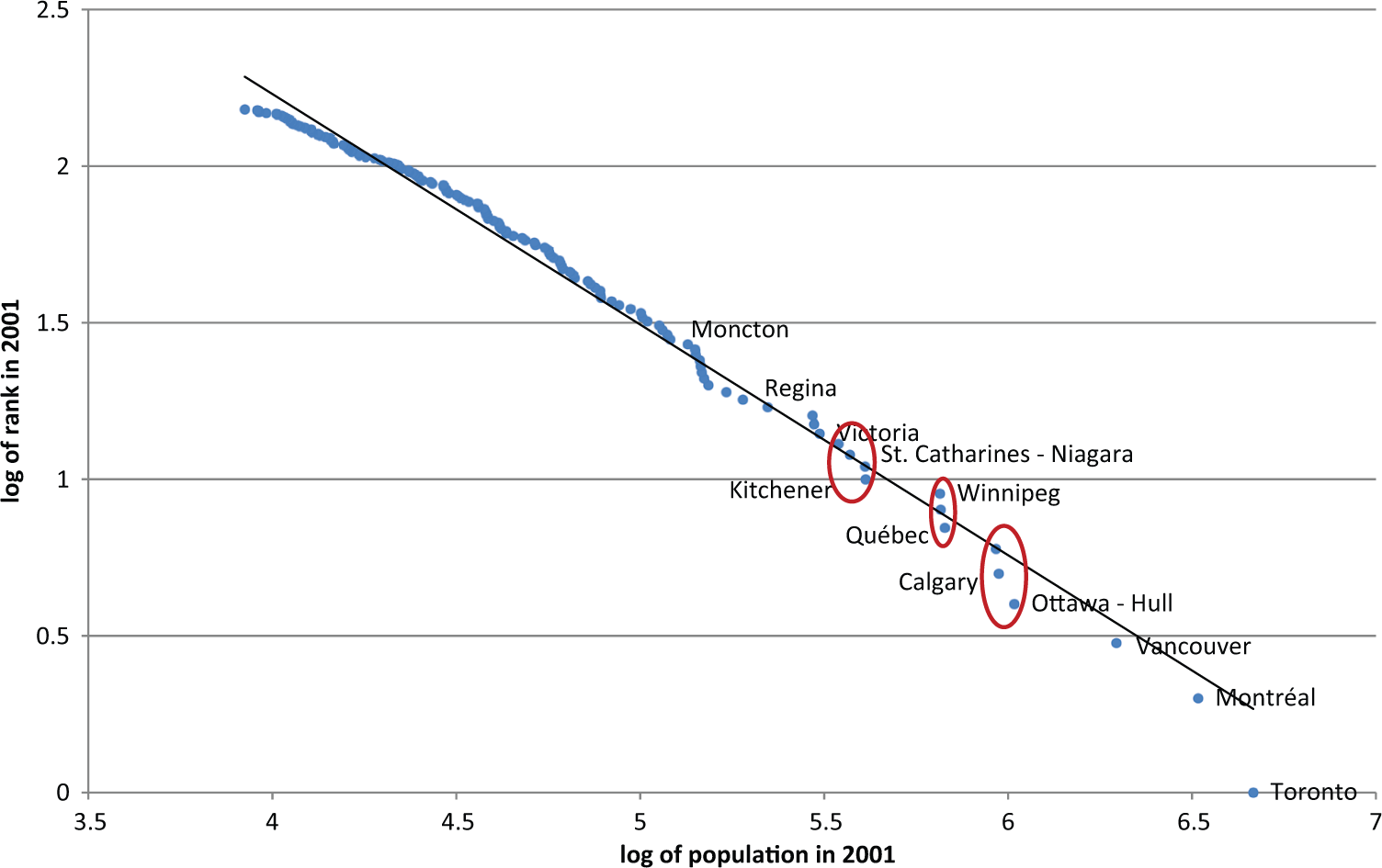
Zipf curve in 2001.

Table 1.

Descriptive statistics of urban areas

Year	average	median	Q1	Q3	Interquartile range
Canada
1971	106,277	28,047	14,625	51,222	36,597
1981	120,185	33,555	15,260	63,337	48,077
1991	138,156	34,030	15,072	72,215	57,142
2001	154,064	35,097	15,990	78,030	62,040
Eastern Canada (n = 102)
1971	119,014	31,055	15,080	78,375	63,295
1981	129,884	33,725	15,385	83,310	67,925
1991	147,730	35,602	14,985	91,385	76,400
2001	162,484	36,100	15,600	94,135	78,535
Western Canada (n = 50)
1971	79,039	18,540	13,125	39,740	26,615
1981	98,732	25,595	14,750	53,800	39,050
1991	116,605	27,935	15,610	60,190	44,580
2001	134,507	32,510	16,125	71,975	55,850

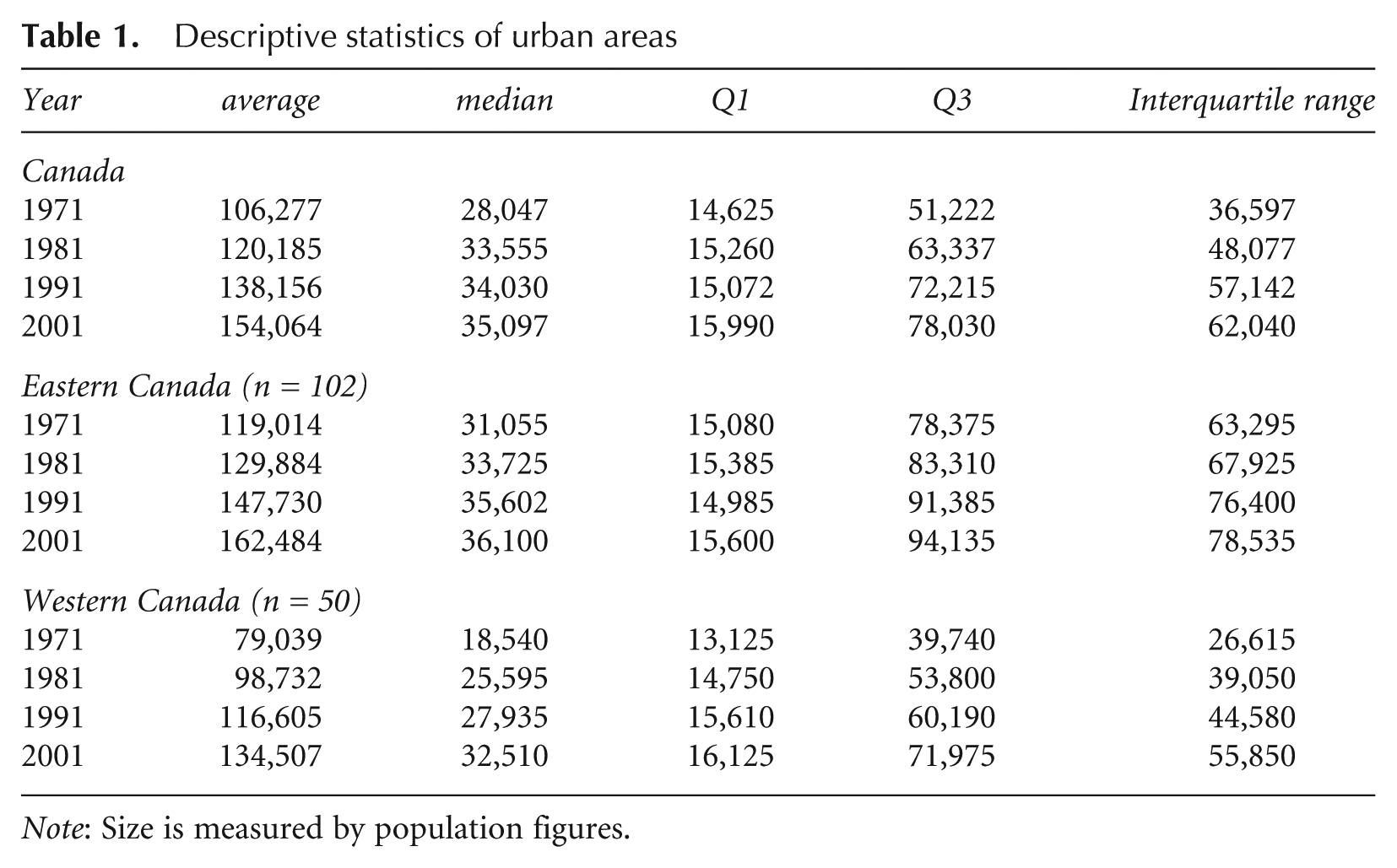
Note: Size is measured by population figures.

The Canadian urban system deviates from Zipf’s law and is tending to move further and further away from it with time (Table 2). In effect, the value of the coefficient over the whole of the period is significantly different from 1 and tends to reduce with time to reach -0.77 in 2001. The estimation of the coefficient and the graph that unveil the scatter-plot of the city-size distribution confirm the macrocephalous and fractured nature of the Canadian urban hierarchical system. As we can see from Figures 2 and 3, this system thus tends to become more and more dominated by the biggest cities (Toronto, Montreal and Vancouver).

Table 2.

Estimation of Zipf’s coefficient for the whole of the Canadian hierarchy (N = 152)

Year	Constant	β	σ(β)	R²	H₀ : β=1
1971	12.47*	−0.81***	0.09	0.98	Rejected
1981	12.61*	−0.81***	0.09	0.98	Rejected
1991	12.44*	−0.79***	0.09	0.98	Rejected
2001	12.22*	−0.77***	0.08	0.98	Rejected

Notes: ***significant at the 99 per cent confidence level; **significant at the 95 per cent confidence level; *significant at the 90 per cent confidence level.

2.3 Growth Patterns within the Canadian Urban Hierarchy

As we saw in the introduction, the theory of random growth supposes that the current size of the city and previous growth have no impact on growth patterns. In order to study the dynamics of growth in population, we will estimate a model whose objective is not to determine growth in population in relation to an unlimited number of variables, but is limited to the most immediate variables for the identification of a city: its size and its growth during the preceding period.

We thus estimate the model

C_{t, t + 10}^{i} = const + α T_{t}^{i} + β C_{t - 10; t}^{i} + ε^{i}

(3)

where, $C_{t; t + 10}^{i} = \log (E_{t + 10}^{i}) - \log (E_{t}^{i})$ is the growth in population for the decade, $T_{t}^{i} = \log (E_{t}^{i})$ population at time t in city i expressed as a logarithm; and $C_{t - 10; t}^{i} = \log (E_{t}^{i}) - \log (E_{t - 10}^{i})$ is growth in population for the preceding period expressed as a logarithm.

The results of this estimation are presented in Table 3. In overall terms, for the three periods, size and previous growth play a role in growth patterns. Thus, these results disagree with those forecasts by theories of random growth. In other words, during the period 1971–2001, growth processes of Canadian urban areas are explained by the size of city and the passage of time.

Table 3.

Results of regression by OLS

	1971–81	1981–91			1991–2001
	(a)	(b)	(c)	(d)	(e)	(f)	(g)
Size	−0.013*	0.028**		0.022***	0.028***		0.003
Previous growth			0.32***	0.303***		0.76***	0.747***
Adjusted R²	0.01	0.11	0.22	0.28	0.11	0.62	0.61
n	150	150	146	148	150	149	149

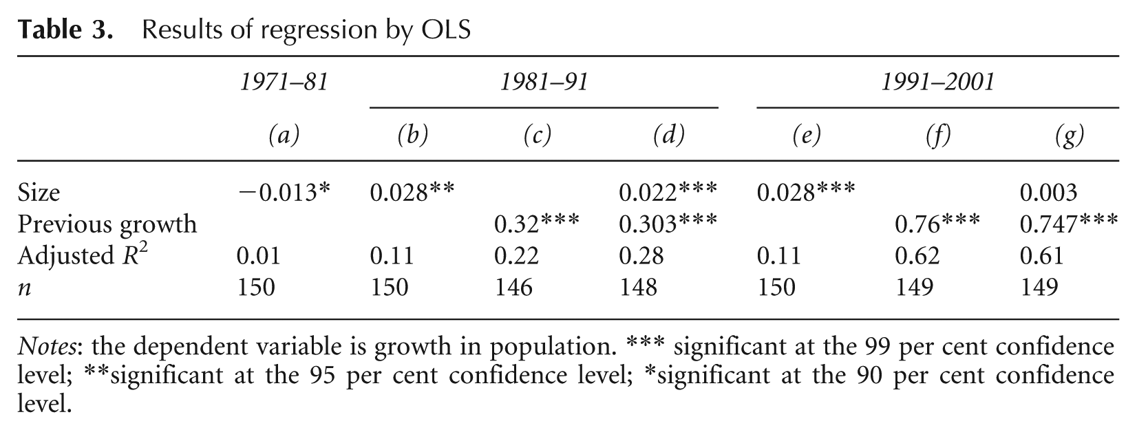
Notes: the dependent variable is growth in population. *** significant at the 99 per cent confidence level; **significant at the 95 per cent confidence level; *significant at the 90 per cent confidence level.

For the first period (1971–81), the role of size in population growth is very weak. Its negative value reminds us that it is the smallest urban areas which tend to grow. For the other two periods (columns b and e), and in particular in the 1980s, the biggest urban areas tended to grow more. Nevertheless, the values of the coefficient remain low.

During the 1980s, the roles of size and previous growth are cumulative and are a good reflection of divergent growth widening the gap between the smallest and the biggest cities. In effect, the significance of the model is weak when the two variables are introduced separately (R² = 0.11 or R² = 0.22) but becomes stronger when the two variables are together (R² = 0.28). However, given the weakness of R², the growth patterns do not seem to be guided only by structural variables but by other incidental factors which are not directly related to the structure of cities per se (Shearmur and Polèse, 2007). When we combine the two variables (column d), the phenomena are cumulative: previous growth leads to more growth and the biggest urban areas get bigger. Moreover, in comparison with the 1970s, we also note a return to growth of the biggest urban areas. Size and previous growth are determining elements in growth patterns.

During the 1990s, the variables are significant with large values but their effects are no longer cumulative (columns e and f). These two dynamics are not cumulative as before, but distinct: whereas the ‘size’ variable is significant alone, it loses its significance when the two variables are introduced (column g). We interpret the absence of cumulative dynamics during the 1990s as a loss of vigour in the process that had been occurring during the 1980s. The growth processes are less polarising because the two variables do not combine to incite growth. On the other hand, the decade of the 1990s is marked by a strong temporal auto-correlation of growth rates. The variable ‘previous growth’ is very strong and very explicative of the model (R² = 0.62, column f). The cumulative and polarising growth dynamics of the 1980s are still very much present. If each period is marked, in its own way, by the events and the context which are specific for that period, it is also the case that the growth dynamics of one period can be marked by the growth dynamics observed during the preceding periods (in our case, the 1980s have marked the 1990s). This indicates that the upheavals which provoked cumulative growth during the 1980s were not completely stabilised in 1990.

The growth patterns were analysed independently of the spatial structure of the urban system. However, this interdependence between cities is another major structural aspect of urban systems (Berry, 1964; Richardson, 1973; Pred, 1977; Favaro and Pumain, 2011; Ioannides and Overman, 2004). Gravitational logic supposes that, the closer two cities are, the more they exchange and become interdependent. Thus a city influences the growth of neighbouring cities and is in turn influenced by these same neighbours. Spatial structure may thus be a third determinist growth factor.

Thus we test the hypothesis of a deterministic process linked to spatial dependence. We base our ideas on the model including the two variables in order to carry out a diagnosis of spatial dependence for each decade (Table 4). When spatial autocorrelation is detected, the estimation by OLS is biased (Anselin, 1988). The test allowing one to choose between two types of model (spatial lag or spatial error model) is the LM statistic (Lagrange multiplier) in its robust version (Anselin, 2003; Florax et al., 2003). We have based the tests on a matrix of the weight of the five nearest neighbours.⁵ These results indicate that the growth of cities in the 1990s is influenced by the growth of the cities around them, which suggests the existence of localised external factors and an effect of diffusion of growth rates. On the other hand, the structural model of the 1970s and 1980s does not appear to be correctly specified. It is thus necessary to specify a model with spatial lag for the 1990s but with auto-correlation of errors for the 1970s and the 1980s.⁶

Table 4.

Cross-correlated autoregressive model and model with spatial auto-correlation of errors, Canada, 1971–2001

	1971–81 (spatial error model) A’	1981–91 (spatial error model) B’	1991–2001 (spatial lag) C’
Size	−0.01	0.023***	0.0012**
Previous growth	—	0.27***	0.69***
δ			0.14*
γ	0.24**	0.18**
R ²	0.06	0.28	0.59
N	150	148	149
Log likelihood	194.227	280.82	330.014
Akaike information criterion	−382.454	−555.65	−652.028
Schwarz criterion	−373.422	−546.65	−640.039
Spatial dependence
Moran’s I	3.44***	2.27**	1.42*
Lagrange multiplier	8.03***	0.24	3.25**
Robust LM	0.25	6.32**	2.22
Lagrange multiplier (error)	8.28***	3.29*	1.22
Robust LM (error)	0.50	9.37***	0.19
Likelihood ratio test (DF = 1)	26.41***	6.44***	2.75**
Tests
Breusch–Pagan	6.34 (0.01)	3.07 (0.08)	2.00 (0.30)

Notes: dependent variable is growth in population. *** significant at the 99 per cent confidence level; **significant at the 95 per cent confidence level; *significant at the 90 per cent confidence level.

The positive and significant values of endogenous spatial lag in the 1990s confirm the important role played by spatial structure (column C’). Localised external factors linked to growth in population thus exist within the Canadian urban system. Including the role of neighbours and diffusion effects enables one to improve the scope of the model. The impact of spatial autocorrelations on growth in population proves to be a variable which is necessary to the understanding of urban systems and the distribution of growth rates.

This model reveals the particular characteristics of the 1970s and the 1980s with respect to growth dynamics. With the model using spatial auto-correlation of errors, the coefficients are always significant and we find a positive spatial auto-correlation of errors. The 1980s are a period of upheavals where a shock which is specific to that period means that all these variables give a poor explanation of the growth of cities. We put forward the hypothesis of a shock during the 1980s with respect to the spatial auto-correlation of errors which emerges. In effect, this poor specification may come from a shock or from a period of upheavals which spreads from one city to another (Baumont et al., 2001). This model, as it is expressed, omits variables which are necessary to an understanding of urban dynamics.

The dynamics of growth of Canadian urban areas thus follow a three-fold deterministic process: morphological (size), temporal (previous growth) and spatial (spatial auto-correlation). The dynamics concerning the role of size and of previous growth on growth in population have not changed.

This first part offers a series of interesting results and directs our work towards the necessity of studying the Canadian urban system at the regional level. In effect, the discontinuity of the distribution of the size of Canadian cities and the existence of a deterministic growth process, implies that in order to understand the whole Canadian urban system it is necessary to look at what happens in each region of Canada (Garmestani et al., 2005, 2007). In the introduction, we pointed out that what is special about Canada is its lack of unity. The geography of the country, as well as its history, leads us to study two potential Canadian urban systems, the east and the west, and to show their similarities and differences.

3. Do Two Canadian Urban Systems Exist?

3.1 Growth Patterns Still Determined by Size and time

In this section, we try to emphasise differences between the eastern and the western parts of the country. We divide the Canadian urban system as follows: the East of Canada, including all the Maritime Provinces, Quebec and Ontario, and the West, including the prairies (Manitoba and Saskatchewan), the northern territories, Alberta and British Colombia. We choose this delineation because the province of Ontario is composed of urban areas that are all located close to Quebec along the Saint-Laurent. There is an ‘urban void’ between the east of Ontario and the West. It creates a gap that underlines a ‘frontier’ between East and West.

Table 1 reveals two different regional setups. The average size is 1.5 times higher in East than in West in 1971. In fact, Figures 2 and 3 reveal that the East of Canada concentrates the biggest urban areas of the country: Montreal, Toronto, Ottawa, Québec. However, there are more important growth processes in the West during the period considered that bring back the average size in the East to only 1.2 times higher in 2001. In fact, there is an increase of 36 per cent of the average size of urban areas in the East, but an increase of 70 per cent in the West. Furthermore, in 30 years, the interquartile range grows by 24 per cent in the East but by 109.84 per cent in the West, while it grows by 70 per cent for the whole country. This means that there are many intradistributional dynamics on the western part.

The dynamics of growth in the East and the West of Canada are presented in Table 5. The growth patterns are similar to those that we found for the whole of Canada: cumulative during the 1980s and stabilisation during the 1990s. This reassures us concerning the stability of our results and also reveals a certain coherence over the whole country. Reasoning on an East/West regional scale does not call into question the logic over the whole country and improves the explanatory scope of the model for the ‘East Canadian’ system. In effect, R² goes from 0.28 to 0.38 during the 1980s and from 0.61 to 0.71 during the 1990s (see Tables 3 and 5). We can, nevertheless, note that there is a difference between the two systems during the 1980s. In the West, city size alone provides a good explanation of growth with R² equal to 0.25 when it is introduced as the only explanatory variable. However, in the East, this single variable accounts for a very small part of the explanation of growth with R² equal to 0.07. Eastern Canada is composed from the biggest urban areas of the country (Montreal and Toronto). Their growth processes are not so important as the growth processes of urban areas such as Vancouver, Calgary. These latter are the biggest urban areas of the West and their growth is important on the period considered. This may be the reason why size is more important in the West than the East to explain the growth.

Table 5.

‘Structural’ model, 1971–2001

	1971–81	1981–91			1991–2001
	(a)	(b)	(c)	(d)	(e)	(f)	(g)
East of Canada 1971–2001 ^a
Size	−0.007	0.02**	—	0.01**	0.02**	—	0.001
Previous growth	—	—	0.58***	0.56***	—	0.77***	0.75***
Adjusted R²	0.002	0.07	0.30	0.38	0.12	0.69	0.71
n	99	100	97	97	100	98	100
West of Canada, 1971–2001 ^b
Size	0.008	0.04**	–	0.025**	0.045**	–	0.006
Previous growth	—	—	0.27**	0.22**	—	0.67***	0.68***
Adjusted R²	0.001	0.25	0.31	0.38	0.26	0.53	0.56
n	47	46	44	44	44	46	47

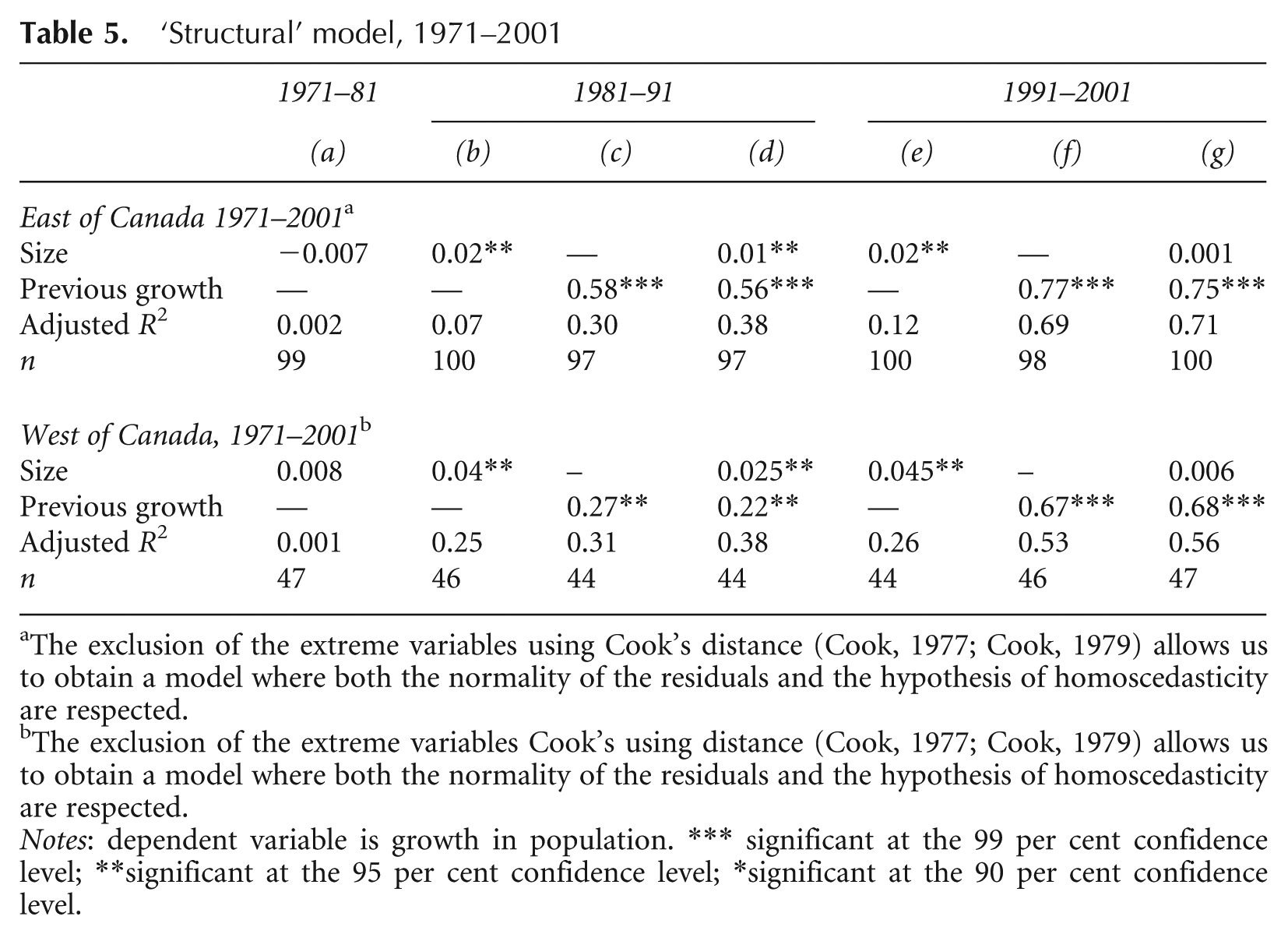
The exclusion of the extreme variables using Cook’s distance (Cook, 1977; Cook, 1979) allows us to obtain a model where both the normality of the residuals and the hypothesis of homoscedasticity are respected.

The exclusion of the extreme variables Cook’s using distance (Cook, 1977; Cook, 1979) allows us to obtain a model where both the normality of the residuals and the hypothesis of homoscedasticity are respected.

3.2 The role of Spatial Autocorrelations in the Distribution of Growth Rates

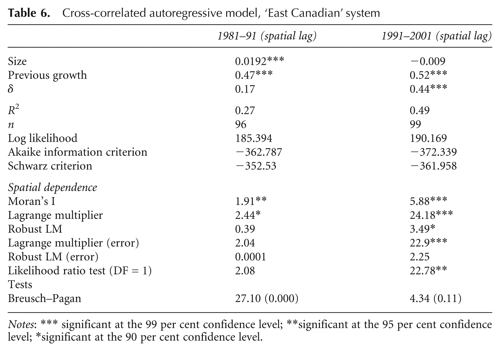
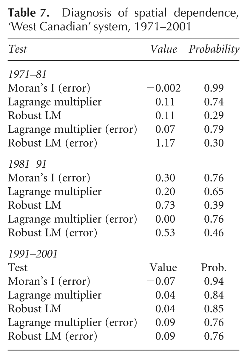
Still using the same logic as in the previous part, we determine the importance of spatial autocorrelations in the distribution of growth rates by carrying out spatial dependency tests on the basis of the model for the cases of East and West Canada. The results are shown in Tables 6 and 7. We maintain the approach using the matrices of the weight of the five closest neighbours.

Table 6.

Cross-correlated autoregressive model, ‘East Canadian’ system

	1981–91 (spatial lag)	1991–2001 (spatial lag)
Size	0.0192***	−0.009
Previous growth	0.47***	0.52***
δ	0.17	0.44***
R ²	0.27	0.49
n	96	99
Log likelihood	185.394	190.169
Akaike information criterion	−362.787	−372.339
Schwarz criterion	−352.53	−361.958
Spatial dependence
Moran’s I	1.91**	5.88***
Lagrange multiplier	2.44*	24.18***
Robust LM	0.39	3.49*
Lagrange multiplier (error)	2.04	22.9***
Robust LM (error)	0.0001	2.25
Likelihood ratio test (DF = 1)	2.08	22.78**
Tests
Breusch–Pagan	27.10 (0.000)	4.34 (0.11)

Notes: *** significant at the 99 per cent confidence level; **significant at the 95 per cent confidence level; *significant at the 90 per cent confidence level.

Table 7.

Diagnosis of spatial dependence, ‘West Canadian’ system, 1971–2001

Test	Value	Probability
1971–81
Moran’s I (error)	−0.002	0.99
Lagrange multiplier	0.11	0.74
Robust LM	0.11	0.29
Lagrange multiplier (error)	0.07	0.79
Robust LM (error)	1.17	0.30
1981–91
Moran’s I (error)	0.30	0.76
Lagrange multiplier	0.20	0.65
Robust LM	0.73	0.39
Lagrange multiplier (error)	0.00	0.76
Robust LM (error)	0.53	0.46
1991–2001
Test	Value	Prob.
Moran’s I (error)	−0.07	0.94
Lagrange multiplier	0.04	0.84
Robust LM	0.04	0.85
Lagrange multiplier (error)	0.09	0.76
Robust LM (error)	0.09	0.76

In the East, the spatial dependence tests reveal that Moran’s I is not significant during the 1970s and that it is not necessary to carry out a cross-correlated autoregressive model or a spatial errors model. On the other hand, for the second and third periods, the value of Moran’s I becomes bigger and bigger and reveals the increasing importance of spatial dependence in the distribution of growth rates in the ‘East Canadian’ urban system. We thus amend the structural model by estimating a cross-correlated autoregressive model for the last two periods.

The two models are not heteroscedastic thanks to the exclusion of extreme values. The results of these two cross-correlated autoregressive models may be summarised in two points. First, isolating the East of Canada from the rest of the territory, in such a way that it forms a completely separate system, does not seem to perturb the dynamics of growth that we have observed for the country as a whole. The patterns relative to size and previous growth are also similar, which tends to confirm our preliminary conclusions about the roles of these variables. Next, this model allows observing the increasing role of spatial autocorrelations in the distribution of growth rates in the ‘East Canadian’ system. Spatial dependence represents a major element in understanding the distribution of the rate of growth in population in the ‘East Canadian’ urban system during the last two decades, but especially in the most recent one. The rupture observed during the 1980s through the use of a spatial auto-correlation of errors at the scale of the whole country no longer appears.

In the West, the tests reveal an absence of spatial auto-correlation of rates of growth in population. These results may be interpreted in different ways. On the one hand, this result may come from a difference in the distribution of urban areas between East and West. The East is much denser, the cities are much closer together, which explains why spatial autocorrelations are much more important, whereas in the West the urban areas are separated by much greater distances which perhaps diminishes the strength of the spatial auto-correlation of growth rates. On the other hand, this result may also reveal the difference in maturity between the ‘East Canadian’ and ‘West Canadian’ urban systems: the ‘East Canadian’ system appears as a mature system in which the proximity to other urban areas operates more and more as a vector of distribution of growth. In contrast, the structure of the spatial autocorrelations of the ‘West Canadian’ system does not (yet) appear as a determining element of growth dynamics. We might imagine that a process of maturation of the ‘West Canadian’ system is currently taking place, not yet leaving an opportunity for spatial autocorrelations to have an effect.

4. Conclusion

This article raises the question of the unity of the Canadian urban system and splitting the Canadian urban system into two—East and West—allows us to identify differences that were not observable when studying the country as a whole. Going further, this article thus raises many further research questions, as much from the point of view of the Canadian urban system (the existence of a cross-border urban system with the US), as of the methods used (the use of non-parametric tools to deepen theoretical and empirical questions).

Footnotes

Funding

This research received no specific grant from any funding agency in the public, commercial or not-for-profit sectors.

Notes

References

Anselin

(1988) Spatial Econometrics: Methods and Models. Dordrecht: Kluwer Academic Publishers.

Anselin

(2003) Spatial externalities, spatial multipliers and spatial econometrics, International Regional Science Review, 26, pp. 153–166.

Baumont

Ertur

Le Gallo

(2001) A spatial econometric analysis of geographic spillovers and growth for European regions, 1980–1995. Laboratoire d’Analyse et des Techniques Economiques, Université de Bourgogne.

Berry

B. J. L.

(1961) City size distribution and economic development, Economic Development and Cultural Change, 9, pp. 573–588.

Berry

B. J. L.

(1964) Cities as systems within systems of cities, Papers in Regional Science, 13, pp. 147–163.

Bosker

Brakman

Garretsen

(2008) A century of shocks: the evolution of the German city size distribution 1925–1999, Regional Science and Urban Economics, 38, pp. 330–347.

Bourne

L. S.

Rose

(2001) The changing face of Canada: the uneven geographies of population and social change, The Canadian Geographer, 45, pp. 105–119.

Brodie

(1997) The new political economy of regions, in: Clement

(Ed.) Understanding Canada: Building on the New Canadian Political Economy. Montréal: McGill-Queen’s University Press.

Champernowne

(1953) A model of income distribution, Economic Journal, 63, pp. 318–351.

10.

Clark

J. S.

Stabler

J. C.

(1991) Gibrat’s law and the growth of Canadian cities, Urban Studies, 28, pp. 635–639.

11.

Cook

R. D.

(1977) Detection of influential observations in linear regression, Technometrics, 19, pp. 15–18.

12.

Cook

R. D.

(1979) Influential observations in linear regression, Journal of the American Statistical Association, 74, pp. 169–174.

13.

Cordoba

J.-C.

(2008) On the distribution of city sizes, Journal of Urban Economics, 63, pp. 177–197.

14.

Davis

Weinstein

(2002) Bones, bombs, and break points: the geography of economic activity, American Economic Review, 92, pp. 1269–1289.

15.

Dobkins

L. H.

Ioannides

Y. M.

(2000) Dynamic evolution of the U.S. city size distribution, in: Huriot

Thisse

J.-F.

(Eds) The Economies of Cities. Cambridge: Cambridge University Press.

16.

Eeckhout

(2004) Gibrat’s law for (all) cities, The American Economic Review, 94, pp. 1429–1451.

17.

Eeckhout

(2009) Reply: Gibrat’s law for (all) cities, The American Economic Review, 99, pp. 1676–1683.

18.

Favaro

J.-M.

Pumain

(2011) Gibrat revisited: an urban growth model including spatial interaction and innovation cycles, Geographical Analysis, 43, pp. 261–286.

19.

Florax

R. J. G. M.

Folmer

Rey

(2003) Specification searches in spatial econometrics: the relevance of Hendry’s methodology, Regional Science and Urban Economics, 33, pp. 1893–1917.

20.

Gabaix

(1999) Zipf’s law for cities: an explanation, The Quarterly Journal of Economics, 114, pp. 739–767.

21.

Gabaix

Ibragimov

(2008) Rank-1/2: a simple way to improve the OLS estimation of tail exponents. Harvard Institute of Economics Research.

22.

Gabaix

Ioannides

Y. M.

(2004) The evolution of city size distributions, in: Henderson

Thisse

J.-F.

(Eds) Handbook of Regional Science and Urban Economics, Vol. 4. Amsterdam: Elsevier Science.

23.

Garmestani

A. S.

Allen

C. R.

Bessey

K. M.

(2005) Time-series analysis of clusters in city size distributions, Urban Studies, 42, pp. 1507–1515.

24.

Garmestani

A. S.

Allen

C. R.

Gallagher

C. M.

(2007) Departures from Gibrat’s law, discontinuities and city size distributions, Urban Studies, 44, pp. 1997–2007.

25.

Gibrat

(1931) Les inégalités économiques. Paris: Librairie du Recueil Sirey.

26.

González-Val

(2010) The evolution of U.S. city size distribution from a long-term perspective (1900–2000), Journal of Regional Science, 50, pp. 952–972.

27.

González-Val

(2011) Deviations from Zipf’s law for American cities: an empirical examination, Urban Studies, 48, pp. 1017–1035.

28.

Ijiri

Simon

(1977) Skew Distributions and Sizes of Business. Amsterdam: North-Holland.

29.

K. S.

Pesaran

M. H.

Shin

(2003) Testing for unit roots in heterogeneous panels, Journal of Econometrics, 115, pp. 53–74.

30.

Innis

H. A.

(1995) Transportation as a factor in Canadian economic history, in: Drache

(Ed.) Staples, Markets and Cultural Change: Selected Essays. Montréal: McGill-Queen’s University Press.

31.

Ioannides

Y. M.

Overman

H. G.

(2004) Spatial evolution of the US urban system, Journal of Economic Geography, 4, pp. 131–156.

32.

Ioannides

Y. M.

Skouras

(2013) US city size distribution: robustly Pareto, but only in the tail, Journal of Urban Economics, 73, pp. 18–29.

33.

Krugman

(1996) Confronting the mystery of urban hierarchy, Journal of the Japanese and International Economies, 10, pp. 399–418.

34.

Le Gallo

Chasco

. (2008) Spatial analysis of urban growth in Spain, 1900–2001, Empiricals Econometrics, 34, pp. 59–80.

35.

Levy

(2009) Comment: Gibrat’s law for (all) cities, American Economic Review, 99, pp. 1672–1675.

36.

Moriconi Ebrard

Pumain

. (1997) City size distribution and metropolisation, Geojournal, 43, pp. 307–314.

37.

Naldi

(2003) Concentration indices and Zipf’s law, Economic Letters, 78, pp. 329–334.

38.

Nishiyama

Osada

Morimune

(2004) Estimation and testing for rank size rule regression under Pareto distribution. Working paper, Kyoto Institute of Economic Research.

39.

Polèse

Denis-Jacob

(2010) Changes at the top: a cross-country examination over the 20th century of the rise (and fall) in rank of the top cities in national urban hierarchies, Urban Studies, 47, pp. 1843–1860.

40.

Pred

(1977) City Systems in Advanced Societies. London: Hutchison.

41.

Richardson

H. W.

(1973) Theory of the distribution of city sizes: review and prospects, Regional Studies, 7, pp. 239–251.

42.

Sharma

(2003) Persistence and stability in city growth, Journal of Urban Economics, 53, pp. 300–320.

43.

Shearmur

Polèse

(2007) Do local factors explain local employment growth?, Regional Studies, 41, pp. 453–471.

44.

Simon

(1955) On a class of skew distribution functions, Biometrika, 44, pp. 425–440.

45.

Soo

K. T.

(2005) Zipf’s law for cities: a cross country investigation, Regional Science and Urban Economics, 35, pp. 239–263.

46.

Soo

K. T.

(2007) Zipf’s law and urban growth in Malaysia, Urban Studies, 44, pp. 1–14.

47.

Watson

A. J.

(2006) Marginal Man: The Dark Vision of Harrold Innis. Toronto: University of Toronto Press.

48.

Harriss

(2010) A spatial and temporal autocorrelated growth model for city rank–size distribution, Urban Studies, 47, pp. 321–335.

49.

Zipf

G. K.

(1949) Human Behavior and the Principle of Least Effort: An Introduction to Human Ecology. Reading, MA: Addison-Wesley Press.