Regional Convergence of Income and Education: Investigation of Distribution Dynamics

Abstract

Recent US studies find that regional education levels diverge and that this can explain the decline of income convergence. The paper challenges the suggested relationship between movements in the distributions of income and education based on Norwegian data. Kernel density functions and Markov chains are applied and a test is undertaken of co-movements in the distributions of education and income. Education levels converge and are equalised across the country, and this process coincides with income convergence. However, the test indicates that transitions in the income and education distributions are basically unrelated. The education level increases in large cities with limited income growth and the income growth is strong in regions with continued low education level.

1. Introduction

Income levels expand hand-in-hand with education levels. The correlation certainly is true at the national level—rich countries have high levels of education. Education increases individual labour productivity and thereby income. In addition, education is assumed to generate positive externalities and then the social return is larger than the private. The cross-country data embody large heterogeneity in institutions and technology, and the relationship between education and income has been investigated in more detail at the regional level. Rauch (1993) innovated the literature by looking at the geographical concentration of the highly educated in cities. Using US metropolitan data he shows that the average level of education has an independent effect on the wage level and thereby confirms the external effect of sharing knowledge. The dynamics of the relationship have not been much studied.

Recent evidence at the regional level is summarised by Gennaioli et al. (2013) and Glaeser and Resseger (2010). ‘Skilled cities’ or ‘smart cities’ (Glaeser and Saiz, 2004; Shapiro, 2006; and Winters, 2011) are seen as engines of growth. Berry and Glaeser (2005) find that education levels diverge across cities in the US and argue that divergence of education levels is related to decline of income convergence. In a study of OECD countries, Wolff (2000) finds convergence in schooling levels and observes that it corresponds to convergence in labour productivity levels. We question the suggested relationship between movements in the distributions of income and education based on Norwegian data.

The dynamic process of accumulating education and income generation is studied for 89 NUTS-4 regions. Based on kernel density functions and Markov transition matrices we find evidence of both income and education convergence among regions. Pearson and likelihood ratio tests are used in the literature to investigate time stationarity. We suggest that the same test design can be used to study co-movements in the distributions of income and education. The test shows that the transitions in the income distribution are independent of whether regions are moving up or down in the distribution of relative education levels.

We see this distribution analysis as an empirical challenge to the literature on education and economic growth. In our data, the education level increases in large cities with limited income growth. Interestingly, the young and highly educated concentrate in large cities with high income levels, but high income growth in the urban regions does not follow. At the other end of the income distribution, growth is strong in regions with a fairly low education level.

Our results should be understood in the context of institutions and characteristics in Norway. This is a welfare state with a large public sector, strong trade unions and income generation influenced by oil and other resource-oriented industries (electric power, salmon). The distribution of income is relatively equal and, as summarised by Oreopoulos and Salvanes (2011), the monetary return to education is lower relative to other high-income countries. The lack of income growth in high-skilled cities may result from a compressed wage structure and low return to education. High income growth in the periphery is probably related to resource-based industries such as salmon farming, electric power generation and oil service.

The distribution analysis is outlined in section 2. Section 3 shows the evidence of regional income convergence in Norway. Section 4 analyses the accumulation of the education level across regions. The relationship between movements in the distributions of income and education is investigated in section 5. Concluding remarks are offered in section 6.

2. Distribution Analysis

We take benefit of long time-series data for education and income and investigate the distributions across 89 NUTS-4 regions in Norway. The regions are aggregated from municipalities and are defined by common labour markets. The average region has about 40,000–50,000 inhabitants. We have collected a measure of regional income per capita based on tax data for the adult population. Personal income in the tax statistic includes wage income, social security and personal capital income. Income from firms is hard to locate at this level of disaggregation, and regional GDP measures are not available. The data cover all years during the period 1972–2008 and it follows that we have 3293 observations of per capita incomes. We measure the level of education in each region as the share of the adult population (16 years and older) with tertiary education, including both short higher education (college level, up to four years in duration) and long higher education (university level, more than four years in duration).¹ The data cover the single year 1970 and all years during the period 1980–2008. In the analysis, the income and education levels are measured relative to the average levels of income and education across all regions in each year.

On average across the 89 regions income per capita grows by 2.7 per cent annually and the share of the adult population with tertiary education increases from 6 per cent to 21 per cent during the past four decades. Yet there are significant differences across regions both with respect to income and education levels. At the beginning of the time-period studied, relative incomes vary from 0.65 to 1.69, while the relative level of education varies from 40 per cent of the average to four times higher than the average. The differences across regions are decreasing over time. In 2008, the relative income levels lie in the range 0.85–1.52, while the share of the adult population with tertiary education varies from 60 per cent of the average to twice the average. The raw data indicate a common convergence of both income and education levels.

We apply distribution analysis to capture heterogeneous processes with different growth paths from different starting-points. There is a large literature applying Markov chain transition probability matrices to study income convergence across regions and countries. Quah (1993a, 1993b, 2001) developed this methodology, more recently applied and extended by Kremer et al. (2001). The basics of the method are presented by Shorrocks (1978). The discussion here relates to the distribution of income, but we also apply the method to investigate the distribution of education levels across regions.

The whole range of relative per capita income is divided into a finite number of N mutually exclusive income groups and in this analysis we follow the convention of working with five groups (N = 5). For each region, we get a sequence of variables describing the income group of that region at time t. The sequences are considered as independent realisations of a single homogeneous Markov chain with finite group space N. The assumption of a finite first-order Markov chain implies that the probability of being in a specific income group at time t only depends on the group of the previous period (and not earlier periods). The probability of moving from group i to group j from period t-1 to period t is described by p_ij(t). The probability is estimated based on observations of how regions move between income groups over time. The number of regions moving from group i to group j from period t-1 to t is measured by n_ij(t). The total number of regions moving from group i from period t-1 to t is measured by n_i(t-1) = ∑_jn_ij(t). The Markov chain can be reduced to a product of five mutually independent multinomial distributions (one for each row i of the transition matrix). For each time-period t, the distribution function is

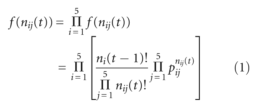
\begin{matrix} f (n_{i j} (t)) = \prod_{i = 1}^{5} f (n_{i j} (t)) \\ = Π_{i = 1}^{5} [\frac{n_{i} (t - 1)!}{Π_{i = 1}^{5} n_{i j} (t)!} Π_{i = 1}^{5} p_{i j}^{n_{i j} (t)}] \end{matrix}

(1)

The transition probabilities can be estimated by maximising the log likelihood of the T multinomials above with respect to p_ij

f (n_{i j}) = Π_{t = 1}^{T} f (n_{i j} (t))

(2)

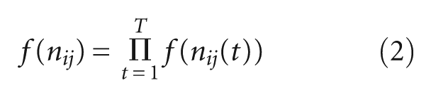
Given the constraint that the sum of p_ij over all j is 1, the maximum likelihood estimator is simply the relative frequency of transitions

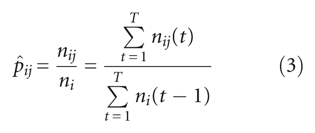
{\hat{p}}_{i j} = \frac{n_{i j}}{n_{i}} = \frac{\sum_{t = 1}^{T} n_{i j} (t)}{\sum_{t = 1}^{T} n_{i} (t - 1)}

(3)

where, n_ij and n_i are the sums of the observed frequencies over all transition periods.

Given the initial distribution of regional income per capita across income groups

h (0) = [h_{1} (0), h_{2} (0), h_{3} (0), h_{4} (0), h_{5} (0)]

where, $\sum_{i} h_{i} (0) = 1$ , the distribution after the first transition period can be calculated as $h (1) = h (0) Ω$ , where Ω is the estimated 5x5 Markov transition matrix. And similarly, the distribution after k transition periods follows as $h (k) = h (0) Ω^{k}$ . Given that the matrix is regular, the distribution converges to the limiting distribution $h^{*} = lim_{k \to \infty} h (0) Ω^{k}$ , which is independent of the initial distribution. This is the ergodic long-run distribution of regional income levels and is estimated based on the Markov chain matrix under the assumption that the transition dynamics remain unchanged.

Pearson and likelihood ratio tests are used in the literature to investigate time stationarity (Geppert and Stephan, 2008; Essletzbichler and Kadokawa, 2010). The test divides the entire sample period into M mutually exclusive and exhaustive sub-periods and compares the transition matrices under each of the M sub-samples with the entire sample. The estimators are obtained based on the distribution function, and Bickenbach and Bode (2003, p. 369) show that the test statistics have an asymptotic χ² distribution. We suggest that the same test design can be used to study co-movements in the distributions of income and education. Instead of looking at different time-periods, we study different education experiences.

The test investigates whether the income transition probabilities are related to the movement in the education distribution. The entire sample of regions is divided into M mutually exclusive and exhaustive sub-samples according to the change in the relative level of education during 1970-2008. The transition matrices under each of the M sub-samples are then compared with the entire sample. The following Pearson (Q) and likelihood ratio (LR) test statistics have an asymptotic χ² distribution with degrees of freedom equal to the number of independent pairwise comparisons

Q = \sum_{m = 1}^{M} \sum_{i = 1}^{5} \sum_{j \in A_{i}} n_{i | m} \frac{{({\hat{p}}_{i j | m} - {\hat{p}}_{i j})}^{2}}{{\hat{p}}_{i j}} ~ a s y χ^{2} (\sum_{i = 1}^{5} (a_{i} - 1) (b_{i} - 1))

(4)

L R = 2 \sum_{m = 1}^{M} \sum_{i = 1}^{5} \sum_{j \in A_{i | m}} n_{i j | m} In \frac{{\hat{p}}_{i j | m}}{{\hat{p}}_{i j}} ~ a s y χ^{2} (\sum_{i = 1}^{5} (a_{i} - 1) (b_{i} - 1))

(5)

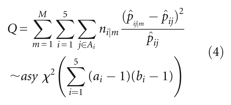
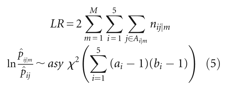
where, A_i is the set of non-zero transition probabilities in the ith row of the transition matrix estimated from the entire sample, while A_i|m is the set of non-zero transition probabilities in the ith row of the matrix estimated from the mth sub-sample. The total number of transitions from group i in sub-sample m and the total number of transitions from group i to group j in sub-sample m are given by n_i|m and n_ij|m respectively. The degrees of freedom are given in the last parenthesis, where a_i is the number of elements in A_i and b_i is the number of sub-samples with a positive number of observations in the ith row.

3. Income Level Convergence

A large literature has analysed income convergence between regions and countries. The estimation of structural convergence equations derived from growth models using various national and regional samples broadly support income convergence. Yet the convergence is heterogeneous, often conditional on other determinants of income, and sometimes restricted to convergence clubs with similar initial conditions. And the convergence is slow, often with a rate of convergence about 2 per cent per year, which implies that the half-life of the convergence process is about 35 years. An influential summary of recent econometric analyses of panel data is given by de la Fuente (2002), including his own analysis of Spanish regions. He concludes that panel analyses of regional data indicate income convergence and with a higher convergence rate than the early static analyses. The use of distribution analysis came as a reaction to the shortcomings of the regression literature and they have given more support to income divergence. Magrini (2009) and Sakamoto and Islam (2008) argue that income convergence understood as reduction in the dispersion of income across regions is best analysed by distribution analysis. Islam (2003) offers an overview of the concepts involved.

To examine how the distribution of regional income per capita develops over time, we compare the estimated kernel density functions for the first year 1972 and the last year 2008, as shown in Figure 1.² The horizontal axis represents income per capita relative to the average level across regions, while the vertical axis gives the density of regions at different relative income levels. The estimated distributions show a clear pattern of convergence over time. Both functions have a single-peak distribution with the majority of regions located close to the average level of income per capita, but the distribution is narrower and more concentrated around the peak in 2008 than in 1972.

Figure 1.

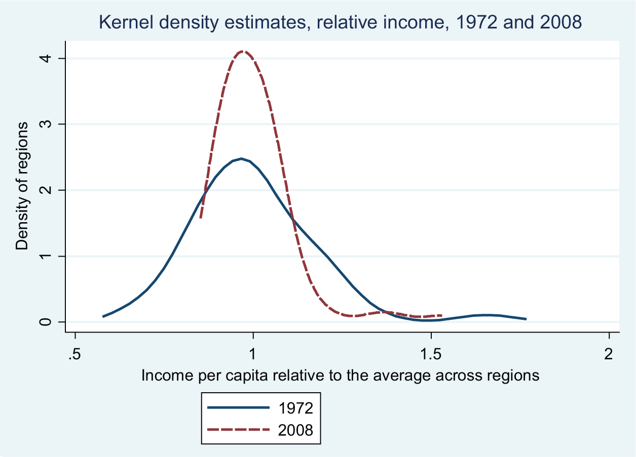
Kernel density estimates, relative income per capita, 89 regions, 1972 and 2008.

In the estimation of Markov chains we report four-year transitions. The pattern is the same for annual transitions, but four-year intervals avoid short-term fluctuations and have more stable transition paths. We follow the convention of discretisation based on a uniform initial distribution of relative incomes across income groups, which gives the following five groups: less than 91 per cent of the average; between 91 per cent and 96 per cent; between 96 per cent and 101 per cent; between 101 per cent and 107 per cent; and more than 107 per cent of the average income across regions. The transition probability matrix is shown in Table 1 and is estimated based on nine four-year transitions and a total of 801 observations. Most of the estimated transition probabilities are significant. As seen from the binomial standard errors given in parentheses, all the diagonal and immediately off-diagonal transition probabilities are significant, while the estimates of the probability of moving two income groups during a four-year period are typically insignificant.

Table 1.

Markov chain transition probability matrix, income per capita, four-year transitions, 1972–2008, 801 observations (binomial standard errors in parentheses)

Income groups	1 ≤ 0.91	2 ≤ 0.96	3 ≤ 1.01	4 ≤ 1.07	5 > 1.07	Observations
1	76.3 (3.4)	23.1 (3.3)	0.6 (0.6)			160
2	15.6 (2.9)	61.3 (3.9)	21.3 (3.2)	1.9 (1.1)		160
3	0.6 (0.6)	19.4 (3.1)	56.3 (3.9)	21.1 (3.2)	0.6 (0.6)	160
4		1.3 (0.9)	24.4 (3.4)	63.1 (3.8)	11.3 (2.5)	160
5			0.6 (0.6)	18.0 (3.0)	81.4 (3.1)	161
Initial distribution	20.0	20.0	20.0	20.0	20.0
Ergodic distribution	15.0	21.9	24.3	23.7	15.1

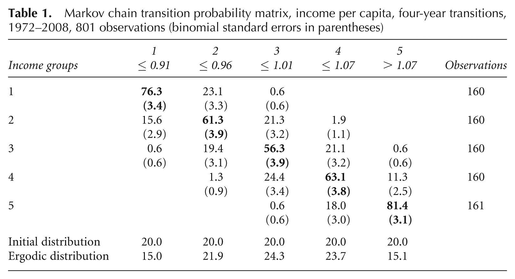
The Markov matrix shows income convergence across regions. The distribution of per capita incomes is tending towards a point mass, rather than towards a two-point distribution. Regions in the lowest income group have 24 per cent probability of moving up during a four-year period and the high-income regions have a 19 per cent chance of moving down the distribution. Regions in income groups 2 and 4 have a higher probability of moving towards the middle of the distribution than towards the respective ends. This pattern is confirmed by the implied ergodic (long-run) distribution given in the last row of the matrix. Regional incomes go from a uniform distribution initially to a normal distribution in the long run. The peak is located around the average income level, with income groups 2–4 (relative income between 91 per cent and 107 per cent of the average), accounting for about 70 per cent of the regions in the long run. The lowest and the highest income groups are reduced from 20 per cent initially to about 15 per cent. The distribution tends to accumulate in the middle, combined with thinning of both the lower and the higher tail, consistent with income convergence. The stationarity of the distribution is addressed by looking at the second eigenvalue of the transition matrix, which is found to equal 0.89. It follows that the distribution converges to a steady state and the asymptotic half life of the process (the time it takes to reach half way to the long-run distribution) equals 5.9 transition periods, which corresponds to about 24 years.

We investigate the time stationarity (constant transition probabilities over time) of the income transition matrix by applying the Pearson (Q) and the likelihood ratio (LR) tests. The transition probabilities are estimated based on nine four-year transitions during 1972–2008. The sample period is divided into three sub-periods, each containing three four-year transitions. The transition matrices for each sub-period are then compared with the full period matrix (given in Table 1). With 28 degrees of freedom, the critical value at the 5 per cent significance level equals 41.3. The test statistics are calculated to Q = 39.4 (probability = 0.07) and LR = 40.1 (probability = 0.06), which means that the null hypothesis of constant transition probabilities over time cannot be rejected. The contributions to the Pearson test statistic from each transition in the three sub-periods show that the differences in transition probabilities are minor. Transition probabilities seem to be constant over time.³

4. Education Level Convergence

The evidence about the development of the regional distribution of education is mixed. Recent studies of US regions find that human capital measured by population shares with college education has diverged during recent decades (Wheeler, 2006; Hammond and Thompson, 2010). A German study looking at shares of high-skilled workers concludes that the regional skill composition has converged over time (Sudekum, 2008).⁴ Yet there are methodological issues involved in the interpretation of results. In the US studies, the dynamic process is considered in terms of absolute changes in college/skill shares. Education divergence comes out because highly educated cities increase their college/skill shares more in percentage points than peripheral regions with low education levels. In our dataset the cities have higher increases in shares with high education in percentage points, but peripheral regions have a higher growth rate of the tertiary share. Our analysis of the education convergence below looks at relative education levels, similar to Sudekum (2008).

The development of the distribution of the education level in the regions is first described by estimated kernel density functions for the first year 1970 and the last year 2008, as shown in Figure 2. The horizontal axis represents the share of the adult population with tertiary education relative to the average share across regions, while the vertical axis gives the density of regions at different relative education levels.⁵ Both distributions have a single peak around the average educational level but, over time, the distribution becomes narrower and the peak more pronounced, indicating convergence with respect to the level of education. Compared with the distribution of income levels, the variations in the level of education are larger across regions.

Figure 2.

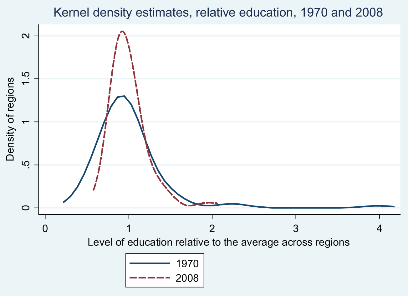
Kernel density estimates, relative level of education, 89 regions, 1970 and 2008.

The robustness of this result is investigated by estimating the kernel using absolute shares of the tertiary educated, similar to Hammond and Thompson (2010). The log shares are presented in Figure 3 and they show the positive shifts in the education share since 1970 and that the distribution has narrowed over time. The standard deviation of the log distribution is lower in 2008 than in 1970. We have calculated the coefficient of variation of the absolute education shares and it is also falling over time. Education divergence is inconsistent with our data, different from the US studies.

Figure 3.

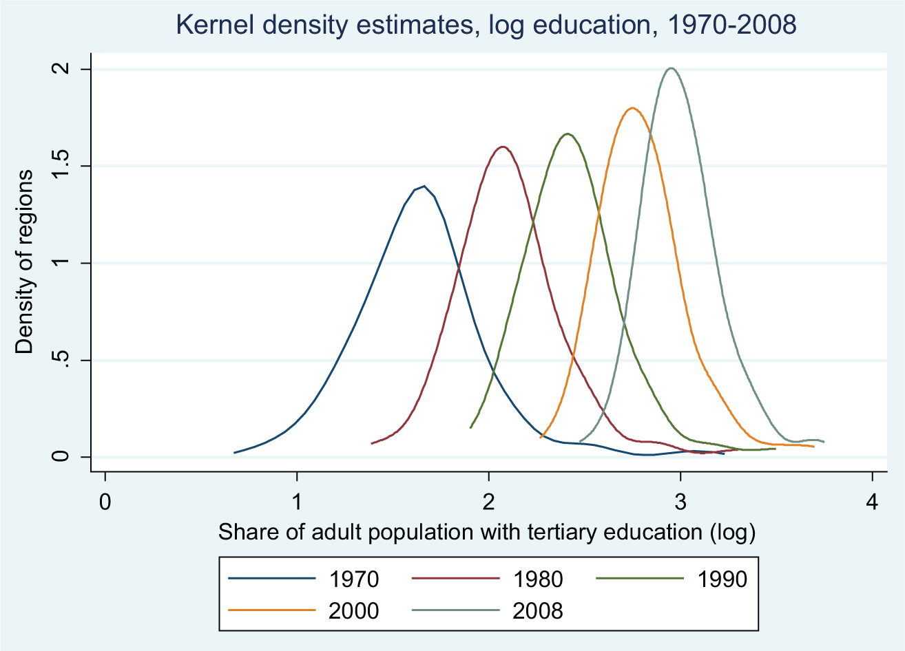
Kernel density estimates, level of education (log), 89 regions, 1970–2008.

Furthermore, we investigate the education dynamics through a Markov chain transition matrix for the period 1970–2008. Since education levels change slowly, we focus on decade transitions and apply the relative education levels in 1970, 1980, 1990, 2000 and 2008. Four transitions and 89 regions imply that transition probabilities are estimated based on 356 observations. Again, we define the range of education groups so that the number of observations is similar across groups. This gives the following five groups: less than 79 per cent of the average educational level; between 79 per cent and 90 per cent; between 90 per cent and 100 per cent; between 100 per cent and 111 per cent; and more than 111 per cent of the average level of education. The Markov matrix with respect to the level of education is given in Table 2. As seen from the binomial standard errors given in parentheses, the estimated transition probabilities are mostly significant.

Table 2.

Markov chain transition probability matrix, level of education, decade transitions, 1970–2008, 356 observations (binomial standard errors in parentheses)

Education groups	1 ≤ 0.79	2 ≤ 0.9	3 ≤ 1.0	4 ≤ 1.11	5 > 1.11	Observations
1	74.7 (5.2)	25.3 (5.2)				71
2	5.6 (2.7)	73.2 (5.3)	19.7 (4.7)	1.4 (1.4)		71
3		13.9 (4.1)	73.6 (5.2)	12.5 (3.9)		72
4			14.1 (4.1)	70.4 (5.4)	15.5 (4.3)	71
5				11.3 (3.8)	88.7 (3.8)	71
Initial distribution	20.0	20.0	20.0	20.0	20.0
Ergodic distribution	3.6	16.2	24.6	23.4	32.2

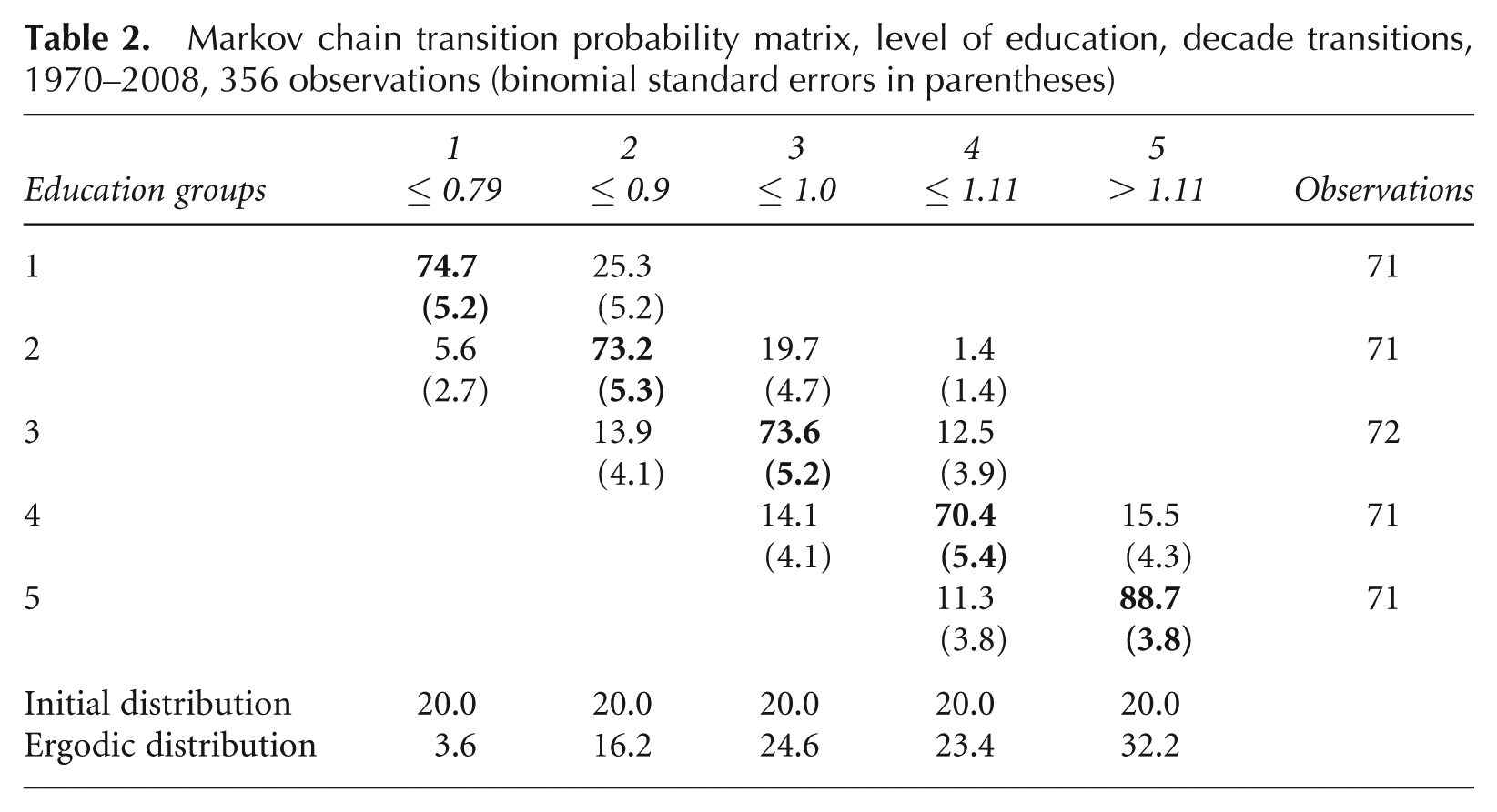
The transition matrix is consistent with the findings from the kernel functions with convergence in educational levels across regions. Regions located in the lowest education group have a 25 per cent chance of moving up the distribution during a 10-year period. Regions in education group 2 are more likely to move towards the middle of the distribution than towards the lower end. Regions in the highest group have good chances of remaining in this group (89 per cent). These dynamics imply a movement towards the top end of the distribution, and education group 5 dominates the long-run distribution with more than 30 per cent of the regions (given in the last row of the matrix). The distribution of educational levels goes from a uniform distribution initially towards a single-peaked distribution, consistent with convergence in education levels, and shows no tendencies towards bimodal twin-peaked distribution. Yet the transition towards the long-run distribution is slow and, based on the second eigenvalue of the matrix, it takes more than 80 years to reach half way to the steady state. The peak at the top end of the distribution means that regions that have reached the highest education group are not likely to leave it again. Kremer et al. (2001) document similar dynamics for the world income distribution.

5. Test of Co-movement in the Distributions of Income and Education

The data analysed thus far show large regional heterogeneity with respect to education and income. The expanding education level in peripheral regions is consistent with convergence in the level of income. In this section, we investigate the relationship between income transitions and the changes in the relative education levels. Is there a systematic pattern of rising educational attainment in regions moving upward in the income distribution?

Direct observation of the distribution across regions in the early 1970s confirms the expected relationship between education level and income level. Small regions in the periphery have low income and education levels, while the large cities have a high share of the adult population with tertiary education and high income levels. Yet the correlation between education level and income level is decreasing over time (raw correlation coefficient 0.80 falling to 0.71) and the correlation coefficient between change in education and change in income is only 0.43. The low correlations indicate that change in education level has not been of much importance for the income transitions.

We investigate co-movements in the distributions of income and education by calculating income transition probability matrices conditioned on the movement in the distribution of education. We rank the 89 regions according to the change in their relative level of education during 1970–2008 and divide the sample into two equal sub-samples (top 50 per cent and bottom 50 per cent). Among the top 45 regions, the relative level of education on average increased by 0.13 (from 0.79 to 0.92). This sub-sample reflects regions with a below-average level of education that are gradually moving up in the education distribution. At the other end, the 44 regions with the largest decrease in relative education are dominated by regions with an above-average level of education that are gradually moving towards the middle of the education distribution (decreasing by 0.13 from 1.21 to 1.08, on average). The estimated Markov matrices for the two sub-samples of regions are shown in Table 3.

Table 3.

Markov chain transition probability matrix, income per capita, four-year transitions, conditioning on the change in the relative educational level during 1970-2008 (binomial standard errors in parentheses)

Income groups	1≤ 0.91	2≤ 0.96	3≤ 1.01	4≤ 1.07	5> 1.07	Observations
Panel a: Top 50 per cent with large increase in the relative educational level (405 observations)
1	78.4 (3.3)	20.9 (3.3)	0.7 (0.7)			153
2	21.9 (4.2)	57.3 (5.0)	18.7 (4.0)	2.1 (1.5)		96
3	1.4 (1.4)	21.9 (4.8)	54.8 (5.8)	20.5 (4.7)	1.4 (1.4)	73
4		1.7 (1.7)	27.1 (5.8)	59.3 (6.4)	11.9 (4.2)	59
5			4.2 (4.1)	25.0 (8.8)	70.8 (9.3)	24
Initial distribution	37.8	23.7	18.0	14.6	5.9
Ergodic distribution	27.0	25.3	22.1	17.5	8.1
Panel b: Bottom 50 per cent with large decrease in the relative educational level (396 observations)
1	28.6 (17.1)	71.4 (17.1)				7
2	6.2 (3.0)	67.2 (5.9)	25.0 (5.4)	1.6 (1.6)		64
3		17.2 (4.0)	57.5 (5.3)	25.3 (4.7)		87
4		1.0 (1.0)	22.8 (4.2)	65.3 (4.7)	10.9 (3.1)	101
5				16.8 (3.2)	83.2 (3.2)	137
Initial distribution	1.8	16.2	22.0	25.5	34.6
Ergodic distribution	1.7	19.3	27.9	31.0	20.1

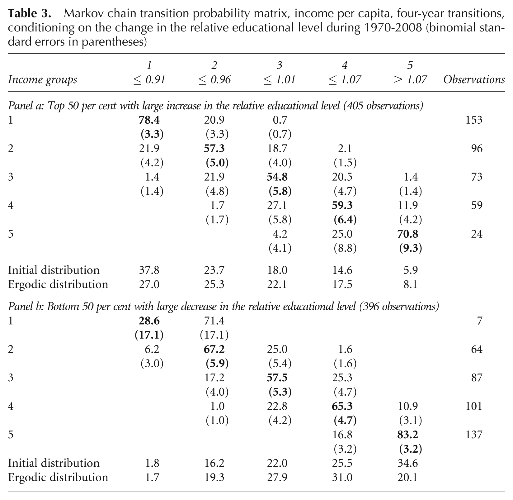
The broad picture is that the development in the relative level of education does not matter much for income transition probabilities. If increased education level is important for upward income transitions, we expect the numbers above the diagonal to be higher in the matrix in panel a than in panel b. Yet the transition probabilities are roughly similar. Whether a region moves up or down in the distribution of relative educational levels does not affect its chances of catching up with respect to income. When it comes to the lowest income group, almost all the regions belong to the sub-sample with a large increase in relative education. A closer look at the data shows that the average increase in the relative level of education is actually higher among regions that remain in the lowest income group than in regions that are able to catch up (0.16 vs 0.12). Rising educational attainment is observed in regions both catching up and falling behind, and is not associated with the income convergence seen in the data. The transition probabilities in the upper end of the distribution are consistent with this view. Income growth has not taken off in high income regions with rising relative education level. And for regions in the sub-sample with a decreasing relative level of education, the decrease is much larger among regions that remain in the top income group than in regions moving down the distribution.

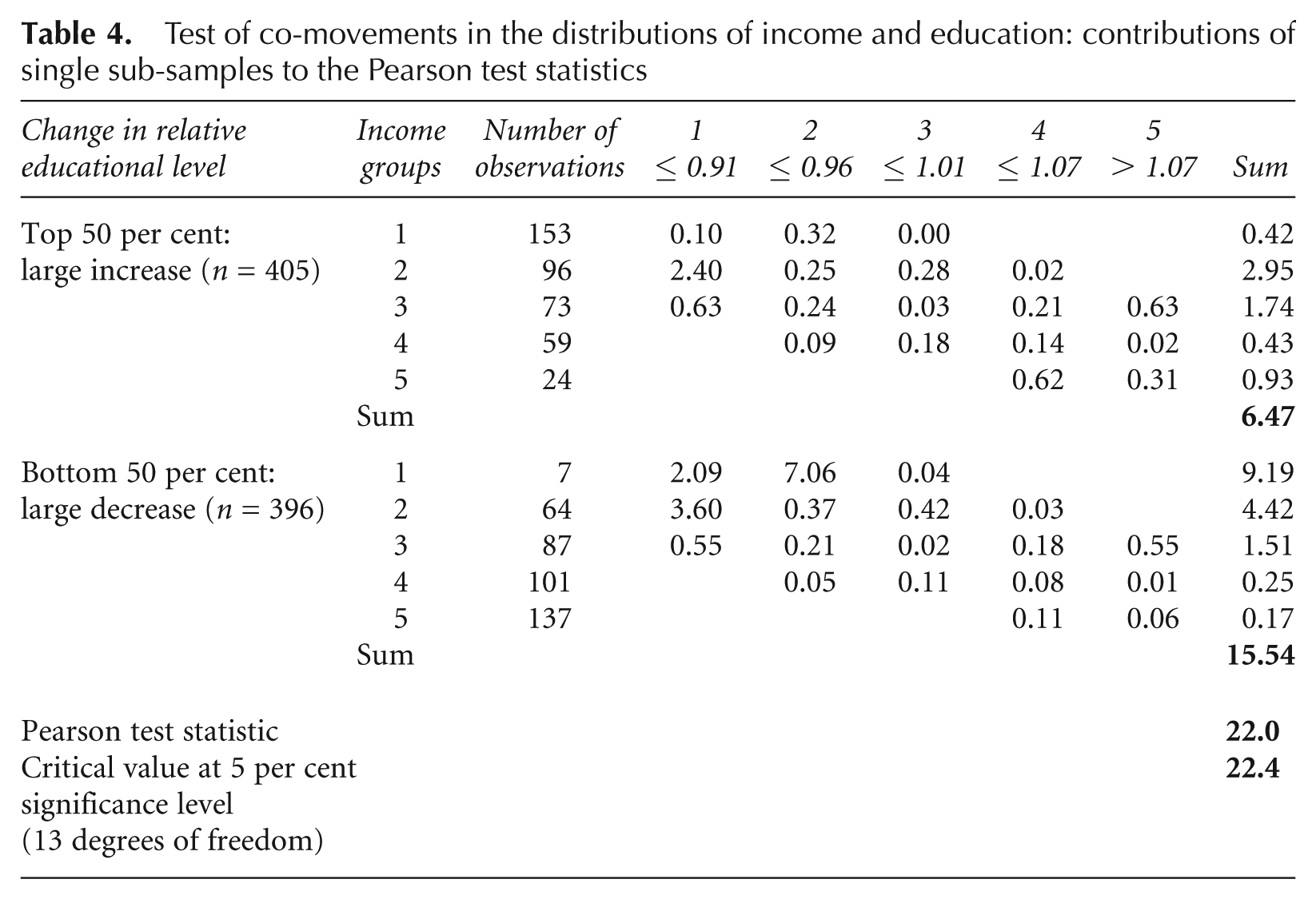
To test statistically for the importance of changes in the relative educational level for the convergence process, we apply Pearson and likelihood ratio tests, as explained in section 2. Comparing the two matrices in Table 3 with the matrix for the entire sample of 89 regions (given in Table 1), we get a test statistic of about 22 for both tests.⁶ With 13 degrees of freedom, the 5 per cent critical value equals 22.4. The null hypothesis of equal transition probabilities across different developments in relative education cannot be rejected. The contributions to the Pearson test statistic from each transition in the two sub-samples are given in Table 4. Differences in transition probabilities are minor and most error terms are well below 0.5. The relatively large test statistic comes from the inaccurate estimates of transition probabilities in the lowest income group in panel b of Table 3, which is based on only seven observations. To sum up, rising educational attainment is not related to income catch-up by low-income regions, and income growth has not taken off in high-income regions with increasing education level.⁷

Table 4.

Test of co-movements in the distributions of income and education: contributions of single sub-samples to the Pearson test statistics

Change in relative educational level	Income groups	Number of observations	1≤ 0.91	2≤ 0.96	3≤ 1.01	4≤ 1.07	5> 1.07	Sum
Top 50 per cent: large increase (n = 405)	1	153	0.10	0.32	0.00			0.42
	2	96	2.40	0.25	0.28	0.02		2.95
	3	73	0.63	0.24	0.03	0.21	0.63	1.74
	4	59		0.09	0.18	0.14	0.02	0.43
	5	24				0.62	0.31	0.93
	Sum							6.47
Bottom 50 per cent: large decrease (n = 396)	1	7	2.09	7.06	0.04			9.19
	2	64	3.60	0.37	0.42	0.03		4.42
	3	87	0.55	0.21	0.02	0.18	0.55	1.51
	4	101		0.05	0.11	0.08	0.01	0.25
	5	137				0.11	0.06	0.17
	Sum							15.54
Pearson test statistic								22.0
Critical value at 5 per cent significance level (13 degrees of freedom)								22.4

In section 4, we referred to the difference between growth rates of education shares and changes of education shares. Instead of focusing on the movement in the distribution of education (the development in a region’s level of education relative to the average), we consider the change in the absolute level of education, measured as the percentage point increase in the tertiary education share of the adult population during 1970–2008. Given this classification of regions, we perform the same analyses and tests as before, and our main results remain. The null hypothesis of equal transition probabilities across sub-samples of regions cannot be rejected. Rising educational attainment is not related to the income convergence movements.

As seen from Table 3, the probability of moving down from the second income group to the lowest group is in fact higher for regions that are catching up with respect to education. Similarly, the probability of remaining in the top income group is highest among regions with large decreases in the relative level of education. These counter-intuitive findings might indicate an importance for the level of education in income transitions. The regions moving up the education distribution typically start from a below-average level of education, while regions moving down the distribution start with an above-average level of education. We investigate the role of the education stock, but find only a weak relationship between education level and movements in the income distribution. Based on the Pearson and likelihood ratio tests, the null hypothesis of equal transition probabilities across sub-samples with different levels of education is not rejected. A more detailed analysis of the top 20 ‘smart cities’ confirms that their income advantage is in decline. This is not surprising given the evidence of income convergence among Norwegian regions (section 3) together with high correlation between income and education.

6. Concluding Remarks

Recent research addresses the divergence of education levels across regions and the relationship to income convergence. We challenge the suggested relationship between movements in the distributions of income and education using Norwegian data. We use kernel density functions and Markov chains, and offer a test of co-movements in the distributions of education and income. Education levels converge as the education level is equalised across the country and this process coincides with income convergence. Yet further investigation of the relationship between education convergence and income convergence shows that transitions in the income and education distributions are basically unrelated.

It is a puzzle that income levels have been catching up in the periphery during a period of stagnation and even of contraction of economic activity. And income levels in ‘smart cities’ with a concentration of the highly educated have not taken off. The background understanding is that the education level increases in large cities with limited income growth and the income growth is strong in regions with a fairly low education level. We cannot rule out the possibility that the results follow from the special characteristics of Norway with its equal distribution of income and resource-oriented periphery. It is of interest to study whether this pattern is similar in other countries; and, in particular, our results raise questions about the limited income growth response to the concentration of human capital in cities.

Footnotes

Acknowledgements

The authors appreciate data handling by Jo Jakobsen, discussions at the 2011 ERSA conference, the 2011 International Atlantic Economic Conference, the NUPI workshop on ‘Barriers to Entry, Internationalisation and Technology’ and at staff seminars at Norwegian University of Science and Technology and the University of California Irvine, and in particular comments from Frank Bickenbach, Hans Bonesrønning, Jan Brueckner, Fredrik Carlsen, Torberg Falch, Amihai Glazer, Holger Görg, Bjarne Strøm, the Editor and two anonymous referees.

Funding

The project is funded by the Demosreg programme of the Norwegian Research Council.

Notes

References

Berry

Glaeser

(2005) The divergence of human capital levels across cities, Papers in Regional Science, 84, pp. 407–444.

Bickenbach

Bode

(2003) Evaluating the Markov property in studies of economic convergence, International Regional Science Review, 26, pp. 363–392.

Essletzbichler

Kadokawa

(2010) The evolution of regional labour productivities in Japanese manufacturing, 1968–2004, Regional Studies, 44(9), pp. 1189–1205.

Fuente

A. de la

(2002) On the sources of convergence: a close look at the Spanish regions, European Economic Review, 46, pp. 569–599.

Gennaioli

La Porta

Lopez-de-Silanes

Shleifer

(2013) Human capital and regional development, Quarterly Journal of Economics, 128(1), pp. 105–164.

Geppert

Stephan

(2008) Regional disparities in the European Union: convergence and agglomeration, Papers in Regional Science, 87(2), pp. 193–217.

Glaeser

E. L.

Resseger

M. G.

(2010) The complementarity between cities and skills, Journal of Regional Science, 50(1), pp. 221–244.

Glaeser

E. L.

Saiz

(2004) The rise of the skilled city, Brookings-Wharton Papers on Urban Affairs, 5, pp. 47–94.

Hammond

G. W.

Thompson

(2010) Divergence and mobility in college attainment across U.S. labor market areas: 1970–2000, International Regional Science Review, 33(4), pp. 397–420.

10.

Islam

(2003) What have we learnt from the convergence debate?, Journal of Economic Surveys, 17(3), pp. 309–362.

11.

Kremer

Onatski

Stock

(2001) Searching for prosperity, Carnegie-Rochester Conference Series on Public Policy, 55, pp. 275–303.

12.

Magrini

(2009) Why should we analyze convergence using the dynamic distribution approach?, Scienze Regionali, 8(1), pp. 5–34.

13.

Oreopoulos

Salvanes

(2011) Priceless: the nonpecuniary benefits of schooling, Journal of Economic Perspectives, 25(1), pp. 159–184.

14.

Quah

(1993a) Empirical cross-section dynamics in economic growth, European Economic Review, 37, pp. 426–434.

15.

Quah

(1993b) Galton’s fallacy and tests of the convergence hypothesis, Scandinavian Journal of Economics, 95, pp. 427–443.

16.

Quah

(2001) Searching for prosperity: a comment, Carnegie-Rochester Conference Series on Public Policy, 55, pp. 305–319.

17.

Rauch

(1993) Productivity gains from geographic concentration of human capital: evidence from the cities, Journal of Urban Economics, 34(3), pp. 380–400.

18.

Sakamoto

Islam

(2008) Convergence across Chinese provinces: an analysis using Markov transition matrix, China Economic Review, 19, pp. 66–79.

19.

Shapiro

(2006) Smart cities: quality of life, productivity, and the growth effects of human capital, Review of Economics and Statistics, 88, pp. 324–335.

20.

Shorrocks

(1978) The measurement of mobility, Econometrica, 46(5), pp. 1013–1024.

21.

Sudekum

(2008) Convergence of the skill composition across German regions, Regional Science and Urban Economics, 38, pp. 148–159.

22.

Wheeler

C. H.

(2006) Human capital growth in a cross-section of US metropolitan areas, Federal Reserve Bank of St. Louis Review, 88, pp. 113–132.

23.

Winters

(2011) Why are smart cities growing? Who moves and who stays, Journal of Regional Science, 51(2), pp. 253–270.

24.

Wolff

(2000) Human capital investment and economic growth: exploring the cross country evidence, Structural Change and Economic Dynamics, 11, pp. 433–472.