Competition over High-income Workers: Job Growth and Access to Labour in Atlanta

Abstract

Access to a large labour pool (labour pooling) leads to local economic concentrations through agglomeration economies. However, these concentrations may be self-limiting by reducing labour availability through competition over high-skill workers. This paper examines whether labour pooling and labour availability of workers with different incomes account for local job growth in the Atlanta metropolitan area between 2000 and 2006. Workers’ income is employed to account for the human capital of workers, including education and skills. It is found that the availability of high-income workers is the only positive significant factor for job growth and the spatial size of the effect is larger than the traffic analysis zone (neighbourhood scale). In contrast, no labour pooling indicators show a positive association with job growth. The finding casts doubt on labour pooling effects at the intraregional level and suggests avenues for further research on local-area agglomeration economies.

Keywords

agglomeration economies Atlanta economic development job growth labour accessibility labour market spatial autocorrelation

1. Introduction

Local economic growth is an important policy objective and agglomeration economies are significant sources for economic growth both locally (neighbourhood to city scale) and regionally (metropolitan scale) (Ciccone and Hall, 1996; Ciccone, 2002; Coffey and Shearmur, 2002; Rice et al., 2006; Rosenthal and Strange, 2008). Among various sources of agglomeration economies, geographical accumulation of human capital contributes to productivity both through access to a large (skilled) labour pool and through informal information spillover (Abel et al., 2012; Ellison et al., 2010; Gabe and Abel, 2001). The labour pooling of high human capital workers helps to drive agglomeration economies (Glaeser and Maré, 2001) and the effect is often local (Glaeser and Kohlhase, 2004; Fu, 2007; Rosenthal and Strange, 2008). Such local-scale agglomeration economies generate local economic concentrations so that some metropolitan areas become polycentric (Coffey and Shearmur, 2002; Lee, 2007).

However, human capital accumulation alone may not attract enterprises if serious competition exists over such workers. Some metropolitan areas move towards dispersion, not polycentricity (Lang, 2003; Lee, 2007), because employment concentration also negatively affects job growth (Combes et al., 2011). Enterprises may avoid employment concentrations because of congestion costs and increased competition over high-skill workers (Combes and Duranton, 2006). Giuliano et al. (2012) empirically support the importance of labour availability. They find that labour availability, not labour pool size, matters to job growth of employment centres in the Los Angeles metropolitan area.

In the empirical assessment of human capital accumulation, researchers often employ educational attainment as an indicator (Rosenthal and Strange, 2008; Glaeser and Resseger, 2010; Abel et al., 2012). However, educational attainment is a limited measurement because workers’ skills affect their wage more than education does (Bacolod et al., 2009) and workers accumulate skills and knowledge over time (Glaeser and Maré, 2001). Industry type or occupation of workers is also used in measuring agglomeration economies within the same industry (Wheaton and Lewis, 2002). However, industry type or occupation may not describe human capital sufficiently because many business skills are transferable across industries (Ellison et al., 2010; Gabe and Abel, 2011).

This paper assesses the effects of labour pooling and labour availability of high- and low-income workers on job growth in the Atlanta metropolitan area, at the traffic analysis zone (TAZ) level (neighbourhood scale) and the US postal system zip code level (sub-regional scale).¹ We test three hypotheses

labour pooling and labour availability of high-income, not low-income, workers have positive associations with job growth.

labour availability of high-income workers is more important to job growth than labour pooling of high-income workers.

labour pooling and labour availability effects are sensitive to the spatial unit of analysis and spatial autocorrelation.

Our paper contributes threefold to the literature. First and most important, we advance the discussion about the human capital factor in the effects of labour pooling and labour availability. Secondly, our analysis considers growth of existing employment centres and places outside centres. Giuliano et al. (2012) explain employment centre growth; however, employment centres capture a minor proportion of jobs in many metropolitan areas (Lang, 2003; Matsuo, 2011) and places outside centres are growing rapidly (Lang, 2003; Phelps, 2004). Thirdly, we consider the spatial scale of the labour pooling and labour availability effects by assessing sensitivity to spatial autocorrelations and spatial scale of the observation unit. The tests are important because the dependent and independent variables we consider may be spatially autocorrelated or have a spatial area of influence larger than the observation unit, leading to biased estimation of the associations. The Atlanta metropolitan area is interesting because it is large enough to observe intrametropolitan variations, and rapidly growing, yet without serious geographical constraints that would limit regional economic development patterns.

As a general measurement of human capital, we employ workers’ earnings. Geographical variations in earnings are often used as an indicator of agglomeration economies (Glaeser and Maré, 2001; Wheaton and Lewis, 2002), but earnings can serve as a uniform measurement of overall human capital. Indeed, a majority of earnings variation is explained by individual characteristics and only a minor proportion of earnings are accounted for by agglomeration economies (Combes et al., 2008). In addition, although levels of earnings differ among industries or occupations, these differences, along with geographical variations in wages, are readily absorbed when earnings categories are aggregated, as in our data.² Data availability is another important advantage of employing earnings as a measurement of human capital. At TAZ level, earnings data are available in the Census Transportation Planning Package (CTPP), while educational attainment is unavailable. For simplicity, we describe workers with high and low earnings as respectively, high- and low-income workers.

A concern may exist that the population of high-income workers itself attracts jobs through a mechanism besides labour accessibility. Specifically, high-income workers may demand more personal service jobs (for example, house cleaning or healthcare), which are often generated in the residential place of high-income workers. We test the direct effect of high-income worker residence to local job growth and find it insignificant. (Results available upon request.)

2. Local Job Growth, Access Labour and Human Capital of Workers

2.1 Agglomeration Economies and Local Job Growth

Literature explores local-scale agglomeration economies and regional-scale agglomeration economies (Rosenthal and Strange, 2003; Fu, 2007; Greenstone et al., 2010). In measuring agglomeration economies, researchers seek three signs: the existence of employment concentrations, high wage and/or rent, and high productivity (Puga, 2010). Among these, employment concentration is often used to measure local-scale agglomeration economies (for example, Ellison and Glaeser, 1999; Rosenthal and Strange, 2003; Duranton and Overman, 2005; Ellison et al., 2010). As Henderson et al. (2001) explain, existence of employment concentrations is theoretical evidence of agglomeration economies. Empirically, jobs are often concentrated in large employment centres (Giuliano and Small, 1991; McMillen and Smith, 2003; among others) and many of these centres persist over time (Giuliano et al., 2007; Redfearn, 2009). Moreover, the spatial structure of intrametropolitan employment distribution affects agglomeration economies: polycentric metropolitan areas are more productive than monocentric counterparts or small cities connected by transport networks (Meijers and Burger, 2010).

The number of jobs, establishments and an index of these are used as measurements of agglomeration economies (for example, Ellison and Glaeser, 1999; Duranton and Overman, 2005; Ellison et al., 2010); however, their derivatives—that is, job growth and plant openings—may primarily account for agglomeration economies. Since the numbers of jobs and enterprises increase over time, the number of jobs may misrepresent agglomeration economies in places such as large declining employment centres or small emerging employment centres. In contrast, job growth and plant openings capture current momentum, occurring where current agglomeration economies outweigh congestion costs.

2.2 Labour Pooling, Labour Availability and Agglomeration Economies

Labour pooling was first proposed as one of the three sources of agglomeration economies: sharing intermediate goods input, labour market pooling and information spillover (Marshall, 1890). Although the original idea of labour pooling focuses on the pool of workers within the same industry, recent research shows that labour pooling effects may cross industrial categories (Ellison et al., 2010; Gabe and Abel, 2011). Instead, large labour pools of high human capital workers are often found to generate agglomeration economies (Glaeser and Resseger, 2010).

While declining transport costs have reduced agglomeration economies from intermediate input sharing (Glaeser and Kohlhase, 2004), labour pooling remains an important source of agglomeration economies. Costs of transporting workers remain high (Glaeser and Kohlhase, 2004) and the size of the accessible labour pool is distributed unevenly within a metropolitan area (Matsuo, 2011). Moreover, the geographical scope of agglomeration economies from human capital (including labour pooling) is local (Fu, 2007). An information spillover effect, another source of agglomeration economies, is found to be both local and regional (McCann and Shefer, 2004; Rosenthal and Strange, 2008; Shearmur, 2012). Although our analysis is limited in controlling for information spillover, employment density and employment size would partially account for potential informal interaction between workers.

Several mechanisms can explain how labour pooling benefits productivity. One is constant access to high-skill workers, which enables firms to more easily adjust employment levels in response to idiosyncratic shocks (Marshall, 1890; Krugman, 1991; Overman and Puga, 2010). Another benefit is better matching between heterogeneous workers and jobs (Helsley and Strange, 1990). A large labour pool also increases a worker’s probability of finding jobs (Coles and Smith, 1998), which improves the quality of matching. This, in turn, allows workers to specialise and increase productivity (Becker and Henderson, 2000).

Despite evidence that local-area agglomeration economies originate from large labour pools, local employment concentration may not occur because it increases competition over workers. Combes and Duranton (2006) illustrate how this competition, or labour poaching, theoretically affects enterprises’ location decisions. If multiple enterprises share a potential labour pool within a region, they risk having internal knowledge stolen by competitors through labour mobility. To prevent workers from moving to competitors, firms must offer workers higher wages, a strategy that may reduce profits. Thus, enterprises may avoid a co-location strategy, despite positive externalities from labour pooling.

Empirically, Giuliano et al. (2012) examine labour pooling and labour availability in explaining the growth of employment centres in Los Angeles between 1990 and 2000. They use various control measures and access measures, including network accessibility (connectivity to other zones within the metropolitan area), total labour force accessibility (labour pooling) and relative labour force accessibility (labour availability). Giuliano et al. (2012) find that network accessibility and relative labour force accessibility have positive associations with the growth of employment centres, while total labour force accessibility does not. Their finding suggests that the labour availability effect (discussed as competition over workers by Combes and Duranton, 2006) may seriously impact job growth. Moreover, ignoring labour availability and network accessibility may cause overestimation of labour pooling effects on local job growth.

A limitation of Giuliano et al. (2012) is they assess only employment centres, not an entire region. Although employment centres persist over time (Giuliano et al., 2007; Redfearn, 2009), there is an undeniable trend of dispersion in many metropolitan areas (Lang, 2003; Lee, 2007). Locations outside the employment centres are growing rapidly (Lang, 2003), possibly by ‘borrowing,’ or receiving the spatial spillovers of, agglomeration economies from neighbouring centres (Phelps, 2004).

2.3 Human Capital of Workers and Agglomeration Economies

The importance of human capital in agglomeration economies is widely recognised (Lucas, 1988; Raunch, 1993). Agglomeration economies through better matching and specialisation are more likely to originate from labour pooling of high-skill, not low-skill, workers. Empirically, agglomeration economies are found in metropolitan areas with high human capital, not in those with low human capital (Glaeser and Resseger, 2010; Abel et al., 2012). At industrial levels, knowledge-intensive industries and occupations enjoy more agglomeration benefits than low-skill ones do (Melo et al., 2009; Gabe and Abel, 2011; Shearmur, 2012). They also cluster regionally (Combes et al., 2008; Gabe and Abel, 2011) and locally (Astrakianaki, 1995; Graham, 2000; Coffey and Shearmur, 2002).

The human capital of workers also affects labour availability. Economic concentration often reduces availability and increases the threat of labour poaching, which discourages further job growth (Combes and Duranton, 2006). Poaching threats are higher for workers with specific skills or expertise because knowledge is partly embodied in workers.

The geographical scope of labour market is also different by human capital of workers. In a heterogeneous labour market, each submarket has different spatial characteristics (van der Laan, 1992; van der Laan and Schalke, 2001). Specifically, the geographical scale of the labour market is larger for high-income and high-educated people than for low-income and low-educated people (Östh, 2007).

3. Research Design and Data

3.1 Job Growth and Accessibility Factors

Local job growth at zone j (GR_j) is associated with access to other zones and workers, and various control variables. Conceptually, the relationships can be described as

{GR}_{j} = f (A_{j}, Z_{j})

(1)

where, A_j is a set of access variables and Z_j is a set of control variables.

As noted earlier, we follow Giuliano et al. (2012) and include three types of accessibility factors: a labour pooling indicator (total labour accessibility, or TLA), a labour availability indicator (relative labour accessibility, or RLA) and a network accessibility indicator. Our analysis further differentiates TLA and RLA by income category of workers to account for human capital of workers. We define each accessibility factor in section 3.4.

Our model controls for factors associated with economic productivity. Following Giuliano et al. (2012), control variables include the number of jobs, employment density, industrial composition and location within the metropolitan area. The size and density of employment may positively or negatively affect job growth because of agglomeration economies and congestion costs associated with the target zones. A large and dense employment concentration may attract more jobs because proximity to other enterprises is another source of agglomeration economies. However, a large and dense employment concentration may not attract jobs because of the high congestion costs of land use and infrastructure.

Industrial composition is another important factor of job growth. Zones with rapidly growing industries naturally grow faster than those with slow growth or declining industries. We control the industrial composition effect by considering the projected growth rate of zone j (PGR_j), which is a weighted average of metropolitan-level job growth rate by industry. Namely

PG R_{j} = \sum_{m} G R^{m} * \frac{e_{j}^{m}}{E_{j}}

(2)

where, GR^m is the average growth rate of industry m in the metropolitan area, $e_{j}^{m}$ is the number of jobs of industry m in zone j in the base year, and $E_{j}$ is the total number of jobs in zone j in the base year.

Last, we control the distance from the central business district (CBD) to account for location within a metropolitan area. Proximity to the CBD may promote job growth through urbanisation economy, while discouraging job growth because of higher rent and congestion.

As a function form, we employ log of growth rate and log of independent variables. The economic literature (for example, Mankiw et al., 1992) often employs log of growth rate in examining rapidly growing periods. Since the Atlanta metropolitan area was rapidly growing during the early 2000s, it is best to analyse log of growth rate, rather than growth rate.³

3.2 Spatial Unit, Scale of Analysis and Spatial Autocorrelations

Methodologically, the spatial scale of the effects and spatial autocorrelation of factors demand serious attention in estimating associations. Many socioeconomic factors are spatially autocorrelated because they are originally spatially contiguous trends. Moreover, the spatial area of influence may be larger than the observation unit, leading to biased estimation in associations. For example, neighbouring zones can ‘borrow’ agglomeration benefits and grow if the spatial size of agglomeration economies is larger than the zone size (Phelps and Ozawa, 2003; Meijers and Burger, 2010). Thus, we must consider spatial autocorrelation in examining association among factors.

We first assess the model with ordinary least square (OLS) and then test sensitivity to spatial autocorrelation. We examine three variations: the spatial autoregressive model (SAR), the spatial Durbin model (SDM) and the spatial error model (SEM). SAR takes into account the spatial autocorrelation of y

y = ρ W y + X β + ε

(3)

where, W is a spatial weight matrix; ρ is a spatial correlation parameter of y; X is a predictors matrix; β is a coefficients vector; and ϵ is an error term. SDM adds spatial autocorrelation of X as follows

y = ρ W y + X β + WX γ + ε

(4)

where, γ is a vector of coefficients of spatially autocorrelated independent variables WX. SEM includes spatial autocorrelation of the error term (equation (5))

\begin{matrix} y = X β + u \\ u = λ W u + ε \end{matrix}

(5)

As spatial weight W may affect the results, we employ a conservative row-standardised matrix of six near neighbours. The contiguity-based matrix is not used due to isolated zones at TAZ-level analysis after removing zones with null values.⁴

Although spatial models account for spatial autocorrelation, our analysis still cannot avoid the modifiable areal unit problem (MAUP). MAUP is a persistent problem for zonal data analysis. Because of spatial aggregation, data and model estimation are sensitive to the size of spatial units (scale problem) and the location of zone boundaries (zoning problem). This holds true even if no spatial autocorrelations exist (Openshaw, 1984). Moreover, the effects of MAUP in multivariate analysis are complicated and the direction of bias is uncertain (Fotheringham and Wong, 1991). Our methods to address MAUP are limited because of data availability; however, we test sensitivity to scale problems by examining both TAZ-level (neighbourhood scale) data and zip code level (sub-regional scale) data.

3.3 Data

The Census Transportation Planning Package (CTPP) for 2000 provides the number of workers by employment location and job distribution by occupation. For transport cost, we employ the estimated AM-peak driving time for 2000, as provided by the Atlanta Regional Commission, a metropolitan planning organisation. AM-peak driving time represents peak-hour labour access, because the single-occupancy vehicle is a dominant commuting mode in the Atlanta metropolitan area (94.1 per cent in year 2000, CTPP 2000). We do not use generalised transport costs because of data unavailability.

Local job growth data are obtained from five-digit zip code business patterns, which record the number of jobs annually since 1994, with fewer missing observations around and after 2000. This data source is preferred over US census data because the severe economic downturn after 2007 may seriously affect the result and because a 10-year period may be too long a timeframe for a business location choice. After assessing three- to seven-year growth, we assessed job growth for the six-year period between 2000 and 2006. We employ this timeframe because the models fit better for longer periods, but performance starts to decline when the recession period is included. The weakness of the data is spatial unit inconsistency with the labour force accessibility assessment. Job growth by zip code is spatially allocated to TAZs, based on the proportion of the area shared by each zone.

Due to unavailable data for travel time and job growth, we employ cross-sectional analysis for this paper; we cannot employ panel analysis to control unobservable local effects.

3.4 Accessibility Measures

Table 1 summarises at TAZ and zip code levels the descriptive statistics of the factors. As described in section 3.1, we consider three types of access factors: network accessibility, TLA and RLA. Network accessibility at TAZ j (NWAcc_j) is measured as follows

NWAc c_{j} = \sum_{i} e^{- β t_{ij}}

(6)

where, t_ij denotes travel time between zones i and j during morning peak; and β is an impedance factor.

Table 1.

Descriptive statistics of factors

		Metro area TAZ(n = 1609; median size 3.28 sq km)		Metro area ZIP(n =129; median size 42.4 sq km)
Access measures	Definition	Median	S.D.	Median	S.D.
NWAcc	Network accessibility	301.2	61.0	309.9	118.5
TLA	Total labour force accessibility	337,232	71,246	3,415,577	2,551,985
RLA	Relative labour force accessibility	470	1309	9001	9764
TLA_U20	Total labour force accessibility to workers whose income in 1999 is under $20,000	103,226	25,124	1,087,856	768,065
RLA_U20	Relative labour force accessibility to workers whose income in 1999 is under $20,000	180.9	383.7	3413.6	2791.9
TLA_O75	Total labour force accessibility to workers whose income in 1999 is $75,000 or higher	37,287	9966	364,236	317,854
RLA_O75	Relative labour force accessibility to workers whose income in 1999 is $75,000 or higher	34.2	200.1	632.6	1441.0
Control measures
GRj	Growth rate between year 2000 and 2006 i.e. the number of jobs in 2006 divided by that in 2000	1.21	0.42	1.19	0.50
lnEmpD00j	Natural log of employment density (per sq km) in zone j	5.31	1.57	5.25	1.81
lnEmp00j	Natural log of employment in zone j	6.55	1.15	9.06	1.31
DistToCBD	Distance from the CBD (km)	28.4	15.1	36.7	22.5
projGR	Projected growth rate between year 2000 and 2006	1.11	0.14	1.12	0.08

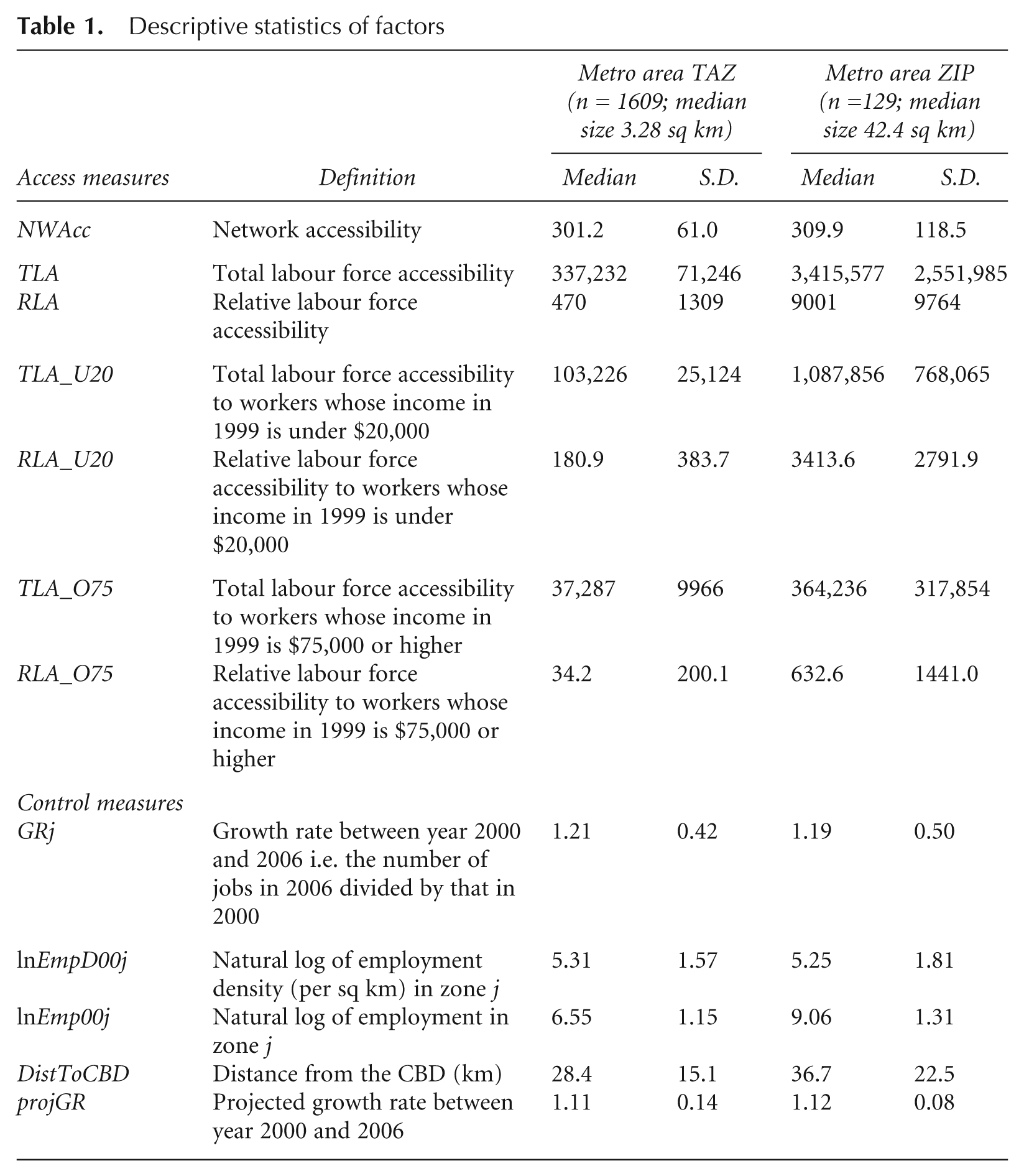
As Fotheringham (1983) demonstrates, there are variations of potential impedance factor, β. We follow Giuliano et al. (2012), using travel time instead of distance as a travel cost measure. Namely, we employ the impedance factor of the inverse of the average commuting time (30 minutes) in the Atlanta metropolitan area.

TLA for TAZ j (TLA_j) equals the sum of the workforce population discounted by travel time

TL A_{j} = \sum_{i} L_{i} * e^{- β t_{ij}}

(7)

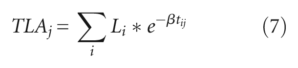
where, L_i stands for the number of workers by residence TAZ i.

In other words, TLA accounts for all workers within an accessible area from employment location. RLA is calculated as TLA discounted by the competition over workers

RL A_{j} = TL A_{j} * \frac{E_{j}}{\sum_{k} E_{k} * e^{- β t_{jk}}}

(8)

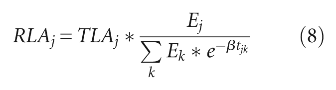
where, E_k is the number of jobs in the TAZ k. Competition over workers is measured as the ratio of the number of jobs in target zone j to the effective number of job opportunities around the zone j.

We next measure TLA and RLA by income category of workers. Based on income category availability (see note 1), we employ earnings in 1999 of less than $20,000 for the low-income category and $75,000 or higher for the high-income category.⁵ The population within each category corresponds to the bottom 30 per cent and top 12 per cent of metropolitan workers. The TLA and RLA differentiated by income categories are defined similarly to TLA and RLA without differentiation (equations (7) and (8)). Namely, TLA to high-income workers is the effective number of high-income workers residing within an accessible area. RLA to high-income workers is TLA to high-income workers discounted by competition over high-income workers (i.e. the number of job opportunities for high-income workers).

Descriptive statistics support our hypothesis that TLA and RLA to high-income workers are different from those to low-income workers (Table 2). TLA and RLA are barely correlated in all cases (between 0.09 and 0.26) and TLA and RLA to high-income workers correlate only moderately with those to low-income workers (0.49 for TLA; 0.68 for RLA). TLA and RLA to high-income workers have obviously different spatial patterns (Figures 1 and 2): TLA to high-income workers is generally higher in the northern suburbs of Atlanta, while zones with high RLA to high-income workers are dispersed in the metropolitan area.

Table 2.

Correlation among TLA and RLA factors

	TLA	RLA	TLA_U20	RLA_U20	TLA_O75	RLA_O75
TLA	1.000
RLA	0.180	1.000
TLA_U20	0.975	0.174	1.000
RLA_U20	0.176	0.925	0.182	1.000
TLA_O75	0.660	0.185	0.489	0.130	1.000
RLA_O75	0.122	0.867	0.086	0.679	0.262	1.000

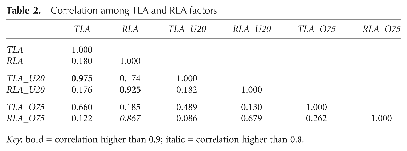
Key: bold = correlation higher than 0.9; italic = correlation higher than 0.8.

Figure 1.

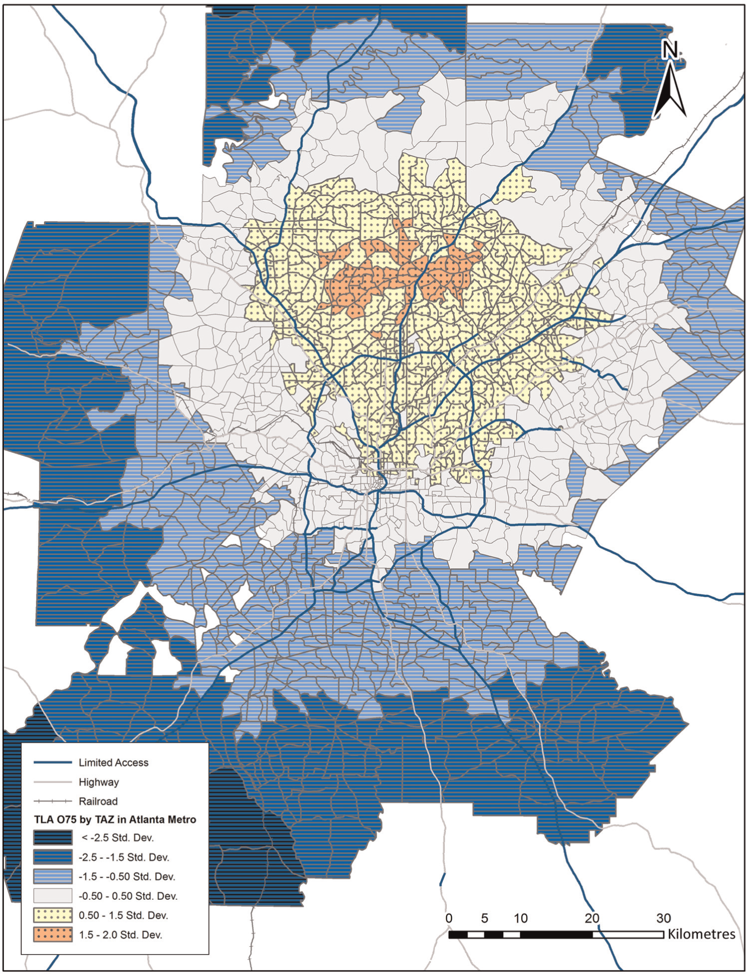
TLA to high-income workers.

Figure 2.

RLA to high-income workers.

4. Job Growth and Labour Force Accessibility

4.1 Job Growth Rate and Labour Force Accessibility Factors in the Atlanta Metropolitan Area

First, we apply our model to examine differences between labour pooling and labour availability effects by worker income category and whether the zone definition affects the outcomes. Table 3 summarises four variations of results: the first two models do not differentiate workers’ income and the latter two examine high- and low-income workers separately. Models 1 and 3 examine each TAZ; models 2 and 4 examine each zip code zone.

Table 3.

OLS results with and without income categories (dependent variable, ln(growth rate))

	OLS	OLS	OLS	OLS
	TAZ	ZIP	TAZ	ZIP
	(1)	(2)	(3)	(4)
Constant	3.08***	−0.0139	10.1***	0.402
	(1.01)	(0.495)	(0.907)	(0.506)
lnEmpD00	−0.0324***	−0.130***	−0.0686***	−0.161***
	(0.00803)	(0.0292)	(0.00929)	(0.0288)
lnEmp00	−0.0528***	−0.0173	−0.0265***	−0.0141
	(0.00839)	(0.0611)	(0.00909)	(0.0573)
lnDistToCBD	0.0971***	0.0665**	0.0285**	0.0612*
	(0.0110)	(0.0340)	(0.0118)	(0.0360)
lnProjGR	−0.00314	−0.628	0.0408	−0.495*
	(0.0369)	(0.307)	(0.0365)	(0.294)
lnNWAcc	0.253	0.134	1.81***	0.148
	(0.171)	(0.0939)	(0.203)	(0.0905)
lnTLA	−0.329**	−0.0574
	(0.154)	(0.0519)
lnRLA	0.00893*	0.105
	(0.00508)	(0.0687)
lnTLA_U20			−1.68***	0.138
			(0.157)	(0.160)
lnRLA_U20			−0.00807	−0.153*
			(0.00855)	(0.0846)
lnTLA_O75			−0.0348	−0.183
			(0.0388)	(0.150)
lnRLA_O75			0.0117	0.214***
			(0.00785)	(0.0612)

Observations	1606	129	1389	129
R ²	0.330	0.376	0.413	0.439
Adjusted R²	0.327	0.340	0.409	0.397

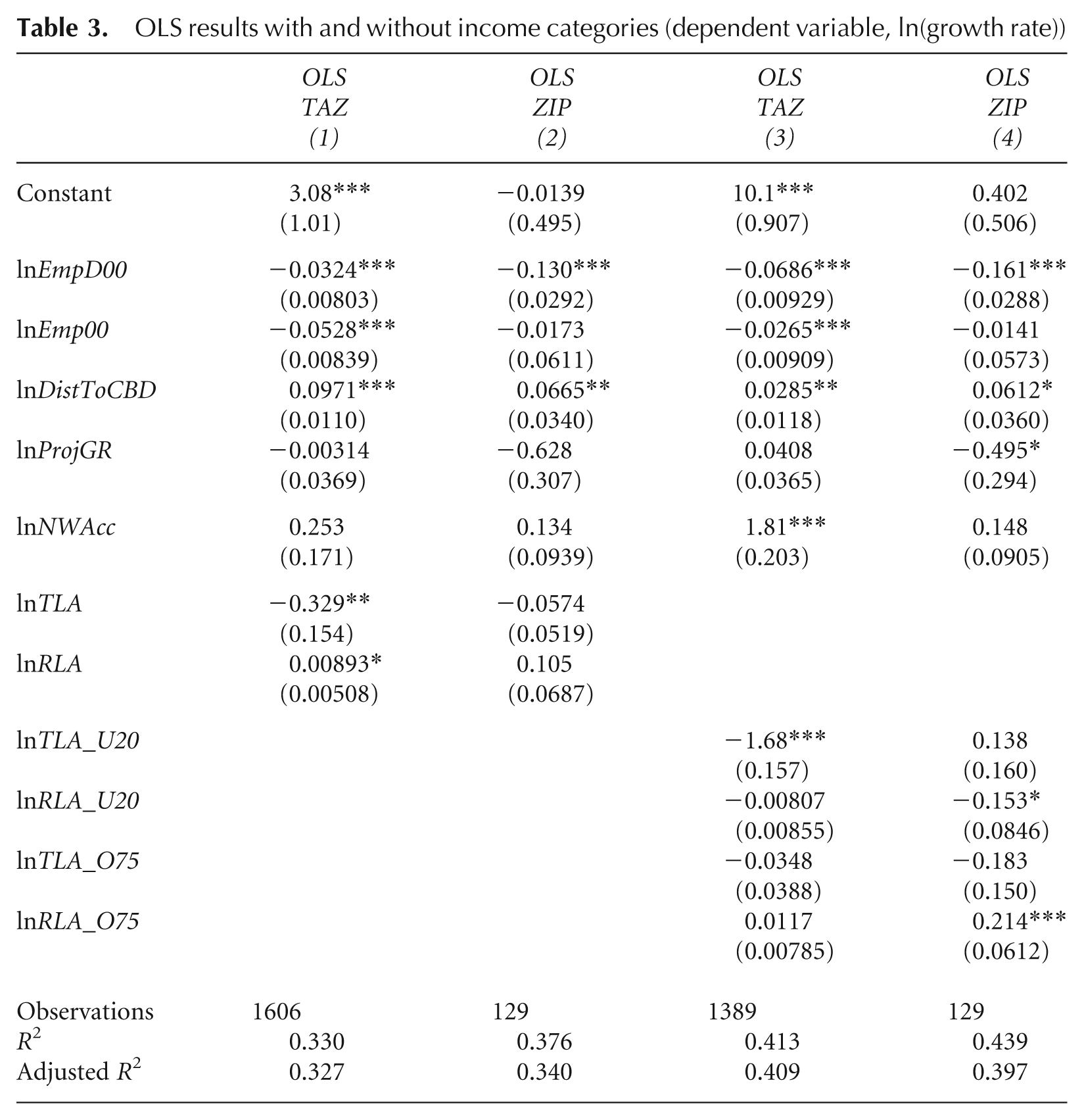
The models illustrate that TLA and RLA have different associations with job growth, and workers’ income category matters. RLA to general workers has a positive association with job growth, while TLA to general workers has a negative association with job growth (models 1 and 2). When the model separates TLA and RLA to high- and low-income workers, the difference becomes more evident. At zip code level, RLA to high-income workers is positive and significant and RLA to low-income workers is negative and significant (model 4). These results not found at TAZ level (model 3). In contrast, none of the TLA factors is positive and significant in models 3 and 4. TLA to low-income workers is negative and significant at TAZ level, yet unobserved at zip code level (i.e. with larger zone size).

The findings suggest three tentative conclusions. First, RLA to high-income worker is positive to job growth. This result strongly supports our hypothesis that the human capital of workers matters, and labour availability is an important job growth factor. Secondly, the spatial area of RLA is larger than TAZ scale and closer to zip code scale. The coefficients are not significant at TAZ level, possibly because the observation unit is too small to capture the effects. Our spatial model in section 4.2 examines if RLA at TAZ level has no association whatsoever to job growth or some indirect association through spatial spillover. Thirdly, TLA is generally irrelevant to job growth (or positive and negative effects cancel out). The negative coefficients of TLA and RLA to low-income workers are not grounded in theory. They may be associated with omitted variable biases.

The impact of network accessibility is positive and significant at the TAZ level when we control income category of workers. The finding is partly consistent with that of Giuliano et al. (2012), which also states the positive association but without controlling for income. Our result suggests that network accessibility contributes to job growth but only at a local scale. At the aggregated zip code level, network accessibility is insignificant, potentially because the effect is local and spatial aggregation renders the indicator meaningless.

Among control variables, the growth rate of jobs has negative and significant associations with employment density and employment. It also has a positive and significant association with distance to the CBD. Negative coefficients for employment and employment density suggest diseconomies of scale exist that discourage job growth. Controlling for access measures, non-centre areas grow faster than employment centres. The consistently positive coefficients of distance to the CBD suggest that employment decentralisation is evident at the metropolitan level even after controlling for employment density and size, industrial organisations and access factors. The projected growth rate is not in the expected positive sign in our analysis (Table 3). The outcome suggests that employment in zones does not grow proportionally relative to that of the initial year of observation; the industrial composition of each zone has changed between 2000 and 2006.

4.2 Controlling Spatial Autocorrelation

The significance of the access measures is sensitive to spatial unit. Part of the problem may originate from spatial autocorrelations. Thus, our models employ spatial models to control spatial autocorrelations. Table 4 compares three spatial models, SAR, SDM and SEM, to determine which to use for data assessment. Table 4 displays ρ and λ, coefficients of the spatial lag of dependent and independent variables, the log likelihood of the model and the Akaike information criterion (AIC). Spatial autocorrelation of a dependent variable is evident when ρ is significant and spatial autocorrelation of an error term is evident when λ is significant.

Table 4.

Model fit comparison of the spatial models

	TAZ			ZIP
	SAR	SDM	SEM	SAR	SDM	SEM
ln(growth rate)
Rho	0.875***	0.898***		0.458***	0.338**
p-value	0.000	0.000		0.000	0.019
Lambda			0.952***			0.501***
p-value			0.000			0.000
Log likelihood	751.6	800.6	604.2	5.54	10.69	3.91
AIC	−1479.3	−1559.2	−1184.3	12.9	20.6	16.2
AIC for linear model	−154.0	−189.8	−154.0	27.4	24.2	27.4

Notes, pp. * significant at 90 per cent level; ** Significant at 95 per cent level; *** significant at 99 per cent level.

Among the models tested, SDM performs the best (the lowest AIC) at TAZ level. At zip code level, SAR performs the best because a larger zone size makes spatial autocorrelation of the independent variables less important, while spatial lag of the dependent variable remains significant. The smaller number of observations also makes it less effective to include additional factors in the model. Table 4 also shows the strength of spatial autocorrelations of the dependent variables. Spatial autocorrelation of log of growth rate at TAZ-level analysis is above 0.85. The high autocorrelation appears to arise from the small size of the zones and the data construction process of job growth. At the zip code level, the spatial autocorrelation of the dependent variable is also significant, but the magnitude is moderate, around 0.35.

Since coefficients of SDM and SAR models are not partial derivatives of factors, we calculate the direct and indirect impacts of independent variables following the recommendation of LeSage and Pace (2009)

\frac{\partial y}{\partial X_{q}} = {(I_{n} - λ W)}^{- 1} (I_{n} β_{q} + W γ_{q})

(9)

where, X_q denotes the qth predictor in the model, and β_q and γ_q are associated parameter coefficients. Note that SAR is the special case of SDM where γ is equal to a zero vector.

Models 1 and 2 in Table 5 describe the results of SDM for TAZ-level analysis and that of SAR for zip code level analysis. RLA to high-income workers now has positive and significant total impacts at both TAZ and zip code levels. At TAZ level, the impact primarily comes from indirect impacts: direct impact is insignificant and indirect impact is significant. At zip code level, RLA to high-income workers is now significant in direct, indirect and total impacts. The effect of RLA to high-income workers is partly internalised (i.e. the indirect impact in TAZ level is partly observed as a direct impact at the zip code level) because of the larger zone size.

Table 5.

Spatial model results (dependent variable, ln(growth rate))

	TAZSDM(1)		ZIPSAR(2)
	Coefficient	p-value	Coefficient	p-value
Direct impact
lnED00	−0.100***	0.000	−0.119***	0.000
lnEmp00	0.011	0.168	−0.052	0.401
lnDistToCBD	0.00564	0.836	0.052	0.158
lnProjGR0006	0.0058	0.846	−0.297	0.309
lnNWAcc	1.17	0.136	0.170*	0.095
lnTLA_U20	−1.28*	0.072	0.212	0.172
lnRLA_U20	−0.00153	0.807	−0.179**	0.036
lnTLA_O75	0.245	0.395	−0.233	0.102
lnRLA_O75	0.00450	0.451	0.230***	0.000
Indirect impact (= spatial spillovers)
W lnED00	−0.0842	0.206	−0.0926**	0.034
W lnEmp00	−0.0548	0.433	−0.041	0.469
W lnDistToCBD	−0.0016	0.960	0.0408	0.256
W lnProjGR0006	0.062	0.871	−0.232	0.374
W lnNWAcc	2.03	0.181	0.133	0.292
W lnTLA_U20	−1.04	0.403	0.165	0.263
W lnRLA_U20	−0.0202	0.790	−0.140	0.120
W lnTLA_O75	−0.401	0.267	−0.181	0.203
W lnRLA_O75	0.152*	0.061	0.179**	0.036
Total impact
lnED00	−0.184***	0.008	−0.211***	0.000
lnEmp00	−0.0441	0.544	−0.093	0.416
lnDistToCBD	0.00401	0.975	0.093	0.178
lnProjGR0006	0.068	0.867	−0.529	0.323
lnNWAcc	3.20**	0.011	0.303	0.168
lnTLA_U20	−2.32**	0.018	0.377	0.192
lnRLA_U20	−0.0217	0.786	−0.319*	0.051
lnTLA_O75	−0.1561	0.495	−0.414	0.125
lnRLA_O75	0.156*	0.066	0.409***	0.001

Notes, pp. * significant at 90 per cent level; ** significant at 95 per cent level; *** significant at 99 per cent level.

The finding supports our OLS model hypothesis: RLA to high-income workers matters for job growth. Moreover, it confirms and strengthens the hypothesis that a TAZ zone is too small to measure RLA effects. We can only observe this effect to high-income workers as an indirect impact because the effect is much larger than the TAZ spatial size. At zip code level analysis, the zone size is now large enough to measure the direct impact from RLA to high-income workers. We still observe indirect impacts, partly because zip code zones are still not large enough to contain all the effects of the zone, and partly because economic activity on the fringes of each zip code zone may interact with neighbouring zones.

In sum, competition over high-income workers occurs in a much larger spatial area than TAZ (neighbourhood scale) and may even be larger than the zip code (sub-regional scale). RLA has a local variation by construction, because it includes competition over workers among neighbouring zones (Figure 2). Neighbouring zones usually enjoy similar size of TLA (Figure 1) and local variations in RLA originate from differences in the number of jobs located in each zone. Our finding suggests that neighbourhood-scale competition is a minor issue. Rather, competition over workers occurs at a larger, sub-regional scale.

Three other factors of labour access—RLA to low-income workers, TLA to high-income workers and TLA to low-income workers—are not positive. No evidence presents for the labour pooling effect based on specific type of workers, even after controlling for spatial autocorrelation. Also, labour availability of low-income workers does not seem to affect job growth. Two negative and significant coefficients—TLA to low-income workers at TAZ level and RLA to low-income workers at zip code level—are not well explained by current theory. These results may suggest omitted variable biases: for example, TLA to low-income workers may indicate a low-quality built environment, which potentially discourages job growth.

Among other factors, employment density and network accessibility are significant in the spatial models. Network accessibility is positive and significant at the TAZ level but insignificant at the zip code level, as observed in the OLS models. The finding confirms that network accessibility is a local factor, and becomes ambiguous in larger zones. Employment density has a negative direct impact, which is economically and statistically significant. Remaining factors—the size of employment, distance to the CBD and projected growth rate—are insignificant in the spatial models. The size of employment and distance to the CBD may have become insignificant possibly because spatial autocorrelation of job growth biases OLS results. The projected growth rate is consistently insignificant in the spatial model, which supports our OLS model conclusion that it does not accurately represent the local growth pattern in the Atlanta metropolitan area.

5. Conclusions

Labour force accessibility has two important aspects, labour pooling (indicated as TLA) and labour availability (indicated as RLA), and their effects are significantly different according to income category of workers. RLA to high-income workers has a positive association with job growth at zip code level, while its effect is fairly indirect at TAZ level. The finding suggests that the spatial extent of the RLA effects is larger than that of TAZ. The positive and significant coefficient of RLA to high-income workers supports our hypothesis that both the human capital of workers and labour availability are important to job growth. In contrast, variations of TLA indicators never appear with positive and significant coefficients, indicating no supportive evidence for the labour pooling effects. The third access factor, network accessibility, is positive and significant at TAZ level but less evident at zip code level. The direct benefit from transport access appears fairly local and aggregating the factor to sub-regional level reduces its explanatory power for job growth.

Methodologically, we scrutinise the spatial scale of the effects by testing sensitivity to spatial scale of observation unit spatial autocorrelation. Small zones, such as TAZ, capture local variations in the effects and reduce concern about spatial aggregations. However, variables observed at small zones are sensitive to spatial autocorrelations and OLS analysis with small-zone data may hide effects that have large spatial spillovers. For example, the positive association between job growth and RLA to high-income worker is not identified in the OLS model at the TAZ level because the effects are sub-regional, not local. Once spatial autocorrelation is controlled, the model can identify the positive and significant indirect impact of RLA to high-income workers at TAZ level.

The result raises a question of whether our finding remains consistent for different places within a metropolitan area or metropolitan areas in different growth stages. Crucial factors for growth may differ based on growth stage. Hence, we propose to explore broader samples to establish a theory that explains associations among TLA, RLA and growth stage of metropolitan areas.

Footnotes

Acknowledgements

The author is grateful for the helpful comments of Hirokazu Ishise.

Funding

This research received no specific grant from any funding agency in the public, commercial or not-for-profit sectors.

Notes

References

Abel

J. R.

Dey

Gabe

T. M.

(2012) Productivity and density of human capital, Journal of Regional Science, 52(4), pp. 563–586.

Astrakianaki

M. A.

(1995) Intra-metropolitan productivity variations of selected manufacturing and business service sectors: what can we learn from Los Angeles?, Urban Studies, 32(7), pp. 1081–1096.

Bacolod

Blum

B. S.

Strange

W. C.

(2009) Skills in the city, Journal of Urban Economics, 65, pp. 136–153.

Becker

Henderson

J. V.

(2000) Intra-industry specialization and urban development, in: Huriot

J.-M.

Thisse

J.-F.

(Eds) Economics of Cities: Theoretical Perspectives, pp. 138–166. Cambridge: Cambridge University Press.

Ciccone

(2002) Agglomeration effects in Europe, European Economic Review, 46(2), pp. 213–227.

Ciccone

Hall

R. E.

(1996) Productivity and the density of economic activity, American Economic Review, 86(1), pp. 54–70.

Coffey

W. J.

Shearmur

R. G.

(2002) Agglomeration and dispersion of high-order service employment in the Montreal metropolitan region, 1981–96, Urban Studies, 39(3), pp. 359–378.

Coles

M. G.

Smith

(1998) Marketplaces and matching, International Economic Review, 39(1), pp. 239–256.

Combes

P.-P.

Duranton

(2006) Labour pooling, labour poaching, and spatial clustering, Regional Science and Urban Economics, 36(1), pp. 1–28.

10.

Combes

P.-P.

Duranton

Gobillon

(2008) Spatial wage disparities: sorting matters!, Journal of Urban Economics, 63(2), pp. 723–742.

11.

Combes

P.-P.

Duranton

Gobillon

(2011) The identification of agglomeration economies, Journal of Economic Geography, 11(2), pp. 253–266.

12.

Duranton

Overman

H. G.

(2005) Testing for localization using micro-geographic data, The Review of Economic Studies, 72(4), pp. 1077–1106.

13.

Ellison

Glaeser

E. L.

(1999) The geographic concentration of industry: does natural advantage explain agglomeration?, American Economic Review, 89(2), pp. 311–316.

14.

Ellison

Glaeser

E. L.

Kerr

W. R.

(2010) What causes industry agglomeration? Evidence from coagglomeration patterns, American Economic Review, 100(3), pp. 1195–1213.

15.

Fotheringham

A. S.

(1983) A new set of spatial-interaction models: the theory of competing destinations, Environment and Planning A, 15(1), pp. 15–36.

16.

Fotheringham

A. S.

Wong

D. W. S.

(1991) The modifiable areal unit problem in multivariate statistical analysis, Environment and Planning A, 23(7), pp. 1025–1044.

17.

(2007) Smart café cities: testing human capital externalities in the Boston metropolitan area, Journal of Urban Economics, 61(1), pp. 86–111.

18.

Gabe

Abel

J. R.

(2011) Agglomeration of knowledge, Urban Studies, 48(7), pp. 1353–1371.

19.

Giuliano

Small

K. A.

(1991) Subcenters in the Los Angeles region, Regional Science and Urban Economics, 21(2), pp. 163–182.

20.

Giuliano

Redfearn

Agarwal

(2012) Network accessibility and employment centers, Urban Studies, 49(1), pp. 77–95.

21.

Giuliano

Redfearn

Agarwal

Zhuang

(2007) Employment concentrations in Los Angeles, 1980–2000, Environment and Planning A, 39(2), pp. 2935–2957.

22.

Glaeser

E. L.

Kohlhase

J. E.

(2004) Cities, regions, and the decline of transport costs, Papers in Regional Science, 83(1), pp. 197–228.

23.

Glaeser

E. L.

Maré

D. C.

(2001) Cities and skills, Journal of Labor Economics, 19(2), pp. 316–342.

24.

Glaeser

E. L.

Resseger

M. G.

(2010) The complementarity between cities and skills, Journal of Regional Science, 50(1), pp. 221–244.

25.

Graham

D. J.

(2000) Spatial variation in labour productivity in British manufacturing, International Review of Applied Economics, 14(3), pp. 323–341.

26.

Greenstone

Hornbeck

Moretti

(2010) Identifying agglomeration spillovers: evidence from winners and losers of large plant openings, Journal of Political Economy, 118(3), pp. 536–598.

27.

Helsley

R. W.

Strange

W. C.

(1990) Matching and agglomeration economies in a system of cities, Regional Science and Urban Economics, 20(2), pp. 189–212.

28.

Henderson

J. V.

Shalizi

Venables

A. J.

(2001) Geography and development, Journal of Economic Geography, 1(1), pp. 81–105.

29.

Krugman

P. R.

(1991) Geography and Trade. Cambridge, MA: MIT Press.

30.

Laan

L. van der

(1992) Structural determinants of spatial labour markets: a case study of the Netherlands, Regional Studies, 26(5), pp. 485–498.

31.

Laan

L. van der

Schalke

(2001) Reality versus policy: the delineation and testing of local labour market and spatial policy areas, European Planning Studies, 9(2), pp. 201–221.

32.

Lang

R. E.

(2003) Edgeless Cities: Exploring the Elusive Metropolis. Washington, DC: Brookings Institution Press.

33.

Lee

(2007) ‘Edge’ or ‘edgeless’ cities? Urban spatial structure in U.S. metropolitan areas, 1980–2000, Journal of Regional Science, 47(3), pp. 479–515.

34.

LeSage

J. P.

Pace

R. K.

(2009) Introduction to Spatial Econometrics. Boca Raton, FL: CRC Press.

35.

Lucas

R. E.

(1988) On the mechanics of economic development, Journal of Monetary Economics, 22(1), pp. 3–42.

36.

Mankiw

G. N.

Romer

Weil

D. N.

(1992) A contribution to the empirics of economic growth, Quarterly Journal of Economics, 107(2), pp. 407–437.

37.

Marshall

(1890) Principles of Economics: An Introductory Volume. London: Macmillan.

38.

Matsuo

(2011) US metropolitan spatial structure and labour accessibility, Urban Studies, 48(11), pp. 2283–2302.

39.

McCann

Shefer

(2004) Location, agglomeration and infrastructure, Papers in Regional Science, 83(1), pp. 177–196.

40.

McMillen

D. P.

Smith

S. C.

(2003) The number of subcenters in large urban areas, Journal of Urban Economics, 53(3), pp. 321–338.

41.

Meijers

E. J.

Burger

M. J.

(2010) Spatial structure and productivity in US metropolitan areas, Environment and Planning A, 42(6), pp. 1383–1402.

42.

Melo

P. C.

Graham

D. J.

Noland

R. B.

(2009) A meta-analysis of estimates of urban agglomeration economies, Regional Science and Urban Economics, 39(3), pp. 332–342.

43.

Openshaw

(1984) Concepts and Techniques in Modern Geography, No. 38: The Modifiable Areal Unit Problem. Norwich: Geo Books.

44.

Östh

(2007) Home, job and space: mapping and modeling the labor market. Geografiska Regionstudier No. 72, Department of Social and Economic Geography, Uppsala University.

45.

Overman

H. G.

Puga

(2010) Labor pooling as a source of agglomeration: an empirical investigation, in: Glaeser

E. L.

(Ed.) Agglomeration Economics. Chicago, IL: University of Chicago Press.

46.

Phelps

N. A.

(2004) Clusters, dispersion and the spaces in between: for an economic geography of the banal, Urban Studies, 41(5/6), pp. 971–989.

47.

Phelps

N. A.

Ozawa

(2003) Contrasts in agglomeration: proto-industrial, industrial and post-industrial forms compared, Progress in Human Geography, 27(5), pp. 583–604.

48.

Puga

(2010) The magnitude and causes of agglomeration economies, Journal of Regional Science, 50(1), pp. 203–219.

49.

Raunch

J. E.

(1993) Productivity gains from geographic concentration of human capital: evidence from cities, Journal of Urban Economics, 34, pp. 380–400.

50.

Redfearn

(2009) Persistence in urban form: the long-run durability of employment centers in metropolitan areas, Journal of Regional Science and Urban Economics, 39(2), pp. 224–232.

51.

Rice

Venables

A. J.

Patacchini

(2006) Spatial determinants of productivity: analysis for the regions of Great Britain, Regional Science and Urban Economics, 36(6), pp. 727–752.

52.

Rosenthal

S. S.

Strange

W. C.

(2003) Geography, industrial organization, and agglomeration, The Review of Economics and Statistics, 85(2), pp. 377–393.

53.

Rosenthal

S. S.

Strange

W. C.

(2008) The attenuation of human capital spillovers, Journal of Urban Economics, 64(2), pp. 373–389.

54.

Shearmur

(2012) The geography of intrametropolitan KIBS innovation: distinguishing agglomeration economies from innovation dynamics, Urban Studies, 49(11), pp. 2331–2356.

55.

Wheaton

W. C.

Lewis

M. J.

(2002) Urban wages and labor market agglomeration, Journal of Urban Economics, 51(3), pp. 542–562.