Urban rapid rail transit and gentrification in Canadian urban centres: A survival analysis approach

Abstract

Despite the existing knowledge that urban rapid rail transit has many effects on surrounding areas, and despite some attempts to understand the links between transit and gentrification, there remain methodological gaps in the research. This study addresses the relationship between the implementation of urban rapid rail transit and gentrification, which is conceived of as an event. As such, an event analysis approach using ‘survival analysis’ is adopted as the statistical analytical tool. It tests whether proximity to rail transit is related to the onset of gentrification in census tracts in Canada’s largest cities. It is found that proximity to rail transit, and to other gentrifying census tracts, have a statistically significant effect on gentrification in two of the three cities analysed. By providing a methodological framework for the empirical analysis of the impact of urban rail transit on gentrification, this paper is a reference for both researchers and transportation planners.

Keywords

gentrification neighbourhood change rapid rail transit survival analysis urban transit

Introduction

Transit is widely recognised as having effects beyond increasing accessibility; however, these effects, including a relationship with the onset of gentrification, are not fully understood. Though this link has been mentioned in the gentrification literature, there is surprisingly little research that examines the relationship explicitly. The studies that exist on transit and gentrification have used definitions of gentrification that differ from those commonly used in the broader literature. One of the implications of this is that the statistical methods employed in these studies are not consistent with the commonly used definitions. We argue that, based on the most common methods of defining gentrification in the literature, the onset of gentrification ought to be thought of as an event, as it is the moment in time when a census tract’s (CT’s) variables are increasing at a rate faster than its surrounding area, which is the moment in time that we are trying to capture in this analysis. As a result, we use ‘survival analysis’, a statistical procedure for analysing data whose outcome variable is ‘time until an event occurs’, to test the relationship between urban rapid rail transit, and the onset of gentrification in Canada’s three largest cities. Both proximity to transit and proximity to other previously gentrifying census tracts appear to have a statistically significant impact on the onset of gentrification. These results follow past findings, but also impart new information about how transit may affect surrounding neighbourhoods.

The questions we address in this paper, and the results presented, provide guidance to researchers and planners as they seek to provide equitable and accessible transit, taking into consideration the implications that the construction of urban rail transit could have on surrounding communities.

The paper starts with a review of existing literature, followed by a description of the cities analysed, and the data and methodology we used to establish which census tracts have experienced the onset of gentrification. We then describe the statistical approach, survival analysis, and the results of the estimated models. Finally, we compare our results with prior research, summarise the contribution this paper represents and offer suggestions for future research.

Literature review

Defining gentrification

While the term ‘gentrification’ has been applied to many different contexts, it is acknowledged by gentrification scholars that for a neighbourhood to have undergone gentrification, it must be considered ‘gentrifiable’: it must have been poor, or ‘working class’, prior to there being a marked change in socio-economic status (Freeman, 2005; Hammel and Wyly, 1996). For an area considered gentrifiable to gentrify, its social status (measured through income, education and percentage of residents in professional occupations) (Filion, 1991; Freeman, 2005; Heidkamp and Lucas, 2006; Ley, 1986) needs to increase faster than that of the city. At the same time, rents and house values should be observed to increase faster than the city as a whole (Hammel and Wyly, 1996; Kahn, 2007; Lin, 2002).

Some authors describe the process as one bringing positive change to neighbourhoods (Freeman, 2005; Vigdor, 2001). Despite these views, the majority of the literature describes adverse effects (Kolko, 2007; Lin, 2002; Newman and Wyly, 2006; Pollack et al., 2010; Rose, 2004; Slater, 2004; Smith and Williams, 1986; Walks and Maaranen, 2008). Negative effects identified range from increases in rents, to displacement of existing residents (Kolko, 2007; Slater, 2004).

There is still some debate as to how this process should be analysed. Using principal component analysis (PCA), Walks and Maaranen (2008) identify not only gentrification, but a variety of forms of ‘upgrading’, where a neighbourhood already considered middle-class experiences an increase in ‘status’ in terms of both income and educational indicators. Owens (2012) uses PCA, but argues that some types of neighbourhood change are not related to gentrification. Stating that research on the topic has been limited in scope, she calls for an expanded terminology (Owens, 2012).

Throughout the gentrification literature, the relationship between accessibility to transit and gentrification has been observed (e.g. Atkinson and Bridge, 2005; Filion, 1991; Skaburskis and Mok, 2006; Walks and Maaranen, 2008). Despite this common acknowledgement there has been little research looking at this question specifically. Before describing this limited literature in detail, it is first necessary to look at how the identification of gentrification has been operationalised.

Identifying gentrification

In studies of gentrification, the basic unit of analysis is the neighbourhood, and census tracts (CTs) are generally used as a proxy (Freeman, 2005; Hammel and Wyly, 1996; Heidkamp and Lucas, 2006; Kahn, 2007; Kolko, 2007; Pollack et al., 2010; Walks and Maaranen, 2008). CTs are used as they are the smallest geographical unit for which the required indicators may be collected.

For a CT to be susceptible to gentrification it must be considered gentrifiable at the beginning of the period of analysis according to the established scholarship on the topic (Freeman, 2005; Hammel and Wyly, 1996; Walks and Maaranen, 2008). Neighbourhoods may be considered to be gentrifiable if the average income of the CT is below the average of the metropolitan area within which it is found (Freeman, 2005; Hammel and Wyly, 1996). Though this way of defining gentrifiable tracts may seem arbitrary, the criteria used follow widely cited texts on the topic. Empirically distinguishing gentrification in an area is more complex. In addition to characteristics of the residents themselves, including increases in levels of educational attainment, incomes, and number of professionals, housing values or rents are also often considered by gentrification experts, since these are important indicators of the gentrification of neighbourhoods (Filion, 1991; Freeman, 2005; Heidkamp and Lucas, 2006; Kahn, 2007; Ley, 1986; Lin, 2002; Pollack et al., 2010; Walks and Maaranen, 2008). Analysis of gentrification is done by measuring whether all of the indicators improve in a given CT at a rate faster than the average rate of the urban region (Freeman, 2005; Owens, 2012). Critical to this is that gentrification is a relative process, gauged against changes in the region being analysed. Also essential is the fact that gentrification is identified by the use of several indicators jointly, meaning that the values of all of the indicators need to increase faster than in the region as a whole – not just one variable – to be considered as having undergone gentrification (Hammel and Wyly, 1996). This methodology is adopted to maintain consistency with the definition earlier described, of gentrification as a change realised in different socio-economic indicators and not just one.

Transit and gentrification

Many studies have focused on the relationship between transit and land value, a common indicator of gentrification (Atkinson-Palombo, 2010; Bajic, 1983; Cervero, 2004, Debrezion et al., 2007; Duncan, 2011; Hess and Almeida, 2007; Immergluck, 2009; Ryan, 1999). Among these studies, regression analysis is the most commonly used method to estimate the effect of proximity to transit on land values while controlling for other explanatory factors.

A study of Toronto’s subway found that property values increased with increased access to the network (Bajic, 1983). In their study of the impacts of light-rail transit on property value, Hess and Almeida (2007) found a marginal appreciation of value related to proximity to transit. Despite these studies, and the aforementioned observations of links between transit and gentrification in the gentrification literature, analysis of this relationship has remained largely overlooked, with only a few studies addressing this topic directly.

In a study of northeastern Chicago, Lin (2002) analysed the link between housing values and proximity to transit stations, and equated higher housing values to the presence of gentrification. Lin estimated regressions of the change in house values for three periods between 1975 and 1990. He observed increased housing values along transit lines for two of the three periods examined, and a pattern of the ‘spreading’ of higher prices away from the shore of Lake Michigan.

The study of Pollack et al. (2010) analysed the demographic progression of ‘transit-rich neighbourhoods’ (TRNs) in 12 metropolitan statistical areas (MSAs) in the US between 1990 and 2000. The authors compared the changes in a number of demographic factors (race, income, car ownership, etc.) between TRNs and the MSA as a whole. They concluded that TRNs more often saw a rise in income, housing values, rent and car ownership greater than in their surrounding MSAs. Twenty-six of the TRNs saw income rise faster than in the MSA as a whole, while in 16 TRNs, the income grew faster across the MSA (Pollack et al., 2010).

In another paper, Kahn (2007) equated increasing home prices and increasing proportion of college graduates with gentrification. Two sets of regressions are estimated. For each of the 14 MSAs included in the study, cross-sectional models of housing values and share of college graduates (as separate models) are estimated. Kahn found that being within a mile of transit stations had differing effects on housing values and the proportion of college graduates, depending upon the city. The second set of regressions looked at the changes in house values and proportion of graduates (in separate regressions) for all MSAs, together, between 1970 and 2000. In these regressions, he found that house prices increased with each additional year that a tract is within a mile of a walk-and-ride station, whereas implementation of park-and-ride stations had the opposite effect.

The three studies previously discussed do not follow conventions in the literature about the definition of gentrification. In particular, none of the three explicitly considers the question of gentrifiability of neighbourhoods in their analyses. Moreover, they only use one variable at a time (and not several jointly) to identify gentrification. Kahn (2007) looks at two indicators in separate regressions, while Lin (2002) only includes one indicator of gentrification in his analysis. Pollack et al. (2010) include a variety of indicators, but they do not address them jointly, looking, rather, at the aggregate trends across their study areas. That gentrification is not defined in a manner consistent with the broader gentrification literature has implications about the appropriateness of the methods used to analyse the effect of transit on gentrification. This is particularly relevant to the Kahn (2007) and Lin (2002) articles that endeavour to estimate the effect of proximity to transit on their indicators of gentrification. Since both of them consider only one indicator in their regressions, and since these indicators are continuous, they can use continuous dependent variable statistical techniques (i.e. OLS). Since the common definition of gentrification requires a CT to have been ‘gentrifiable’, and to have had several indicators all improve more than the metropolitan region as a whole in the same period, gentrification should not be described as a continuous variable. Instead, the process of gentrification is more appropriately thought of as an event – characterised as a variable that takes a value of 1 if a CT is observed to have undergone gentrification, and a value of 0 if it has not.

The research presented here builds on the transit and gentrification literature by employing a conventional definition of gentrification, and by using a more suitable statistical technique in the context of gentrification as an event – that is, survival analysis.

Study areas: Montreal, Toronto and Vancouver

The study areas for this research are the census metropolitan areas (CMAs) of Montreal, Toronto and Vancouver in Canada. Toronto is the largest with a total population of 5.1 million residents in 2006 (Statistics Canada, 2007). The Toronto subway first opened in 1954 and in 2006 had 69 stations extending 70 kilometres through the City of Toronto (TTC, 2012). The limits of the City of Toronto in 2001 were used as the boundaries of the area of analysis as they encompass the entirety of the subway system, and the CT identifiers for the area were available from 1961 to 2006.

Montreal, Quebec, is the second largest Canadian city with a CMA population of 3.6 million (Statistics Canada, 2007). The Montreal metro was inaugurated in 1966 (Clairoux, 2001). As of 2006 it consisted of 68 stations on the island of Montreal which were opened in 11 increments between 1966 and 1988. Off island metro stations were excluded because they opened after the end of the study period (to the north), and because CT boundaries consistent over time were unavailable for the study period (to the south).

The third city is Vancouver, which as of 2006 had a CMA population of 2.1 million (Statistics Canada, 2007). Vancouver’s SkyTrain opened its first stations in 1986. By 2006 it had 32 stations along 68.7 kilometres of track. It provides service to the city of Vancouver as well as four adjacent municipalities (Metro Vancouver, 2010). An additional line has opened since 2006, but as the study period ended in 2006, that line is not included here.

Defining the boundaries of the study for Vancouver was more challenging than for the other cities since there was no obvious delineation. As such, three conditions were used to establish the study area boundaries: any CTs separated from the SkyTrain by water were eliminated, and CTs with population densities lower than the tenth percentile were not considered in the analysis.

In initial analyses of Vancouver, when all CTs were included in the analysis, several outlying CTs appeared as having undergone gentrification. These CTs had high percentages of agricultural employment and had low population densities. It was clear that what was being observed was not gentrification, but rather urbanisation. Since gentrification is characterised as taking place in urban areas (see e.g. Freeman, 2005; Ley, 1986), it was deemed necessary to restrict the analysis to ‘urban’ CTs. Various population density thresholds were tested to do this. The lowest threshold that most effectively included urban areas, while excluding predominantly agricultural and other non-urban CTs on the fringes of the city was the tenth percentile population density.

Finally, CTs were also excluded if they were not a part of the contiguous area of ‘urban’ CTs, that is, if they were separated from the SkyTrain by areas with less than the tenth percentile population density.

Data used

To establish whether the process of gentrification is occurring, empirical studies use census data to distinguish changes in neighbourhoods, or CTs (Freeman, 2005; Hammel and Wyly, 1996; Heidkamp and Lucas, 2006; Kahn, 2007; Kolko, 2007; Pollack et al., 2010; Walks and Maaranen, 2008). Indicators of gentrification used in the past to measure the process include demographic statistics: population; household, family and individual income; education levels; persons in professional occupations; household structure (number of children in a household); and racial and ethnic composition, particularly in studies conducted in the USA. Indicators related to housing and location are also taken into account as statistics on the number of housing units, housing tenure and age; housing costs, both the value of homes and costs of rent (list compiled from: Filion, 1991; Freeman, 2005; Hammel and Wyly, 1996; Pollack et al., 2010; Walks and Maaranen, 2008).

As such, census data were aggregated to the CT level and were collected from Statistics Canada, and CT boundaries were normalised to the first year in each of the study periods. Study periods for the cities varied depending on when their respective transit systems first came into operation. For Montreal the first year of census data used is 1961, five years before the first stations opened. In Vancouver the study period only begins in 1981 as the SkyTrain was first inaugurated in 1986. Comparable census statistics were not available for Toronto for 1951 (the census before the subway opened in 1954), and as such the study period for Toronto is the same as Montreal: 1961–2006. Missing variables in 1966 and 1976 led them to be excluded from the analysis so the full dataset for both Montreal and Toronto includes census years 1961, 1971, 1981, 1986, 1991, 1996, 2001 and 2006.

In addition to census statistics, other data were used as control variables in the survival models of gentrification. These were chosen based on those that have been identified in previous literature as being associated with gentrification. They included the straight-line distance from the centroids of each CT to the nearest transit station for every year from the time that the first stations were opened. Although network distance would also have been a useful measurement, Hess and Almeida (2007) found that the perceived proximity to transit, as measured by the straight-line distance, had a greater effect on property values of surrounding neighbourhoods – one important indicator of gentrification. Past studies have explored the idea that gentrification is related to the distance from the CBD (Filion, 1991; Kahn, 2007; Lin, 2002; Walks and Maaranen, 2008). As such, distance from CT centroids to the centroid of the CBD was used as an additional control variable. Distance to the CBD is included in this – and previous – analyses of gentrification primarily because it serves as a proxy for proximity to tertiary employment (Walks and Maaranen, 2008). It would be interesting to explicitly include measures of accessibility to employment, but employment data by CT were not available at this scale for the full study period. Another characteristic of gentrifying neighbourhoods mentioned in the literature is the presence of older housing stock with the architectural character desired by ‘gentrifiers’ (Filion, 1991; Ley, 1986; Walks and Maaranen, 2008). To control for this, the census variable ‘proportion of pre-1946 housing’ in each CT was used.

Many authors refer to the urban amenities that draw gentrifiers to the desirable neighbourhoods (Heidkamp and Lucas, 2006; Helms, 2003; Ley and Dobson, 2008; Lin, 2002; Smith and Williams, 1986; Walks and Maaranen, 2008). Often urban amenities refer to commercial districts that cater to middle and upper income residents (Smith and Williams, 1986). Since these attributes were impossible to track over the period of this study they were excluded from this analysis, but both parks and proximity to water, viewed as urban amenities (Heidkamp and Lucas, 2006; Helms, 2003; Ley and Dobson, 2008; Lin, 2002), were included as control variables.

In order to integrate these variables in the analysis the distance was measured from the centroid of each CT to the nearest large park (defined by the authors as any park equal to or exceeding 50,000 square metres) or major body of water (lake, river or ocean). Though the size of the park may seem arbitrary, some boundary was necessary to ensure that the parks included in the study were of a certain importance and therefore more likely to represent a recognised amenity such as Montreal’s Mount-Royal or Vancouver’s Stanley Park. The final variable that was included was the distance from the centroid of each CT to the centroid of the nearest CT that had experienced gentrification. This variable draws on one of the determinants of gentrification highlighted by Kolko (2007): the spillover effect of proximity to higher income neighbourhoods.

Another type of variable that would ideally have been included in the analysis would identify public policies or investments associated with the construction of the transit infrastructure that may have influenced the onset of gentrification. Obtaining such information is difficult, and as a result it was not incorporated into the analysis, but was left as a suggestion for further research.

Methodology

Identifying gentrification

In order to conduct a statistical analysis of the effect of urban rail transit on gentrification, it is necessary to identify CTs that could be considered gentrifiable, and those that have actually undergone gentrification over the study period.

To establish whether a CT was gentrifiable average family income of a census tract and number of degrees per capita were assessed, both of which needed to be lower than the CMA average. If this was the case for a CT, then the CT in question was included in the sample for the statistical analysis. The full list of indicators used in the identification of the onset of gentrification included:

average monthly rent;

proportion of people in professional occupations;

percentage of owner-occupied dwellings;

average family income; and

number of degrees per capita.

For a CT to be considered to have undergone gentrification, all of these indicators had to have experienced an improvement in that CT greater than the average change experienced in those indicators for the CMA in the same year. Additionally, the CT needed to be considered gentrifiable in the preceding census year in the dataset (i.e. to have undergone gentrification in 1971, it must be considered gentrifiable in 1961). Table 1 summarises how many CTs were included for each CMA, how many of those were considered gentrifiable according to our criteria, and how many ultimately underwent gentrification. Figure 1 highlights the census tracts that were considered gentrifiable at any point during the study period, and those that were observed to have gentrified in Toronto. Figure 2 shows the results of the gentrification analysis for Montreal. Figure 3 depicts the gentrifiable and gentrifying tracts in Vancouver.

Table 1.

Gentrifiable and gentrifying tracts for all cities.

City	CTs included in study	Gentrifiable CTs	Gentrifying CTs
Montreal	291	220 (75%)	86 (29%)
Toronto	248	165 (67%)	71 (29%)
Vancouver	143	101 (71%)	19 (13%)

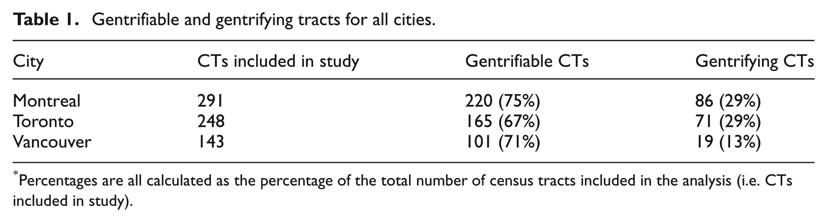
Percentages are all calculated as the percentage of the total number of census tracts included in the analysis (i.e. CTs included in study).

Figure 1.

Gentrifiable and gentrifying census tracts in Toronto (1961–2006).

Figure 2.

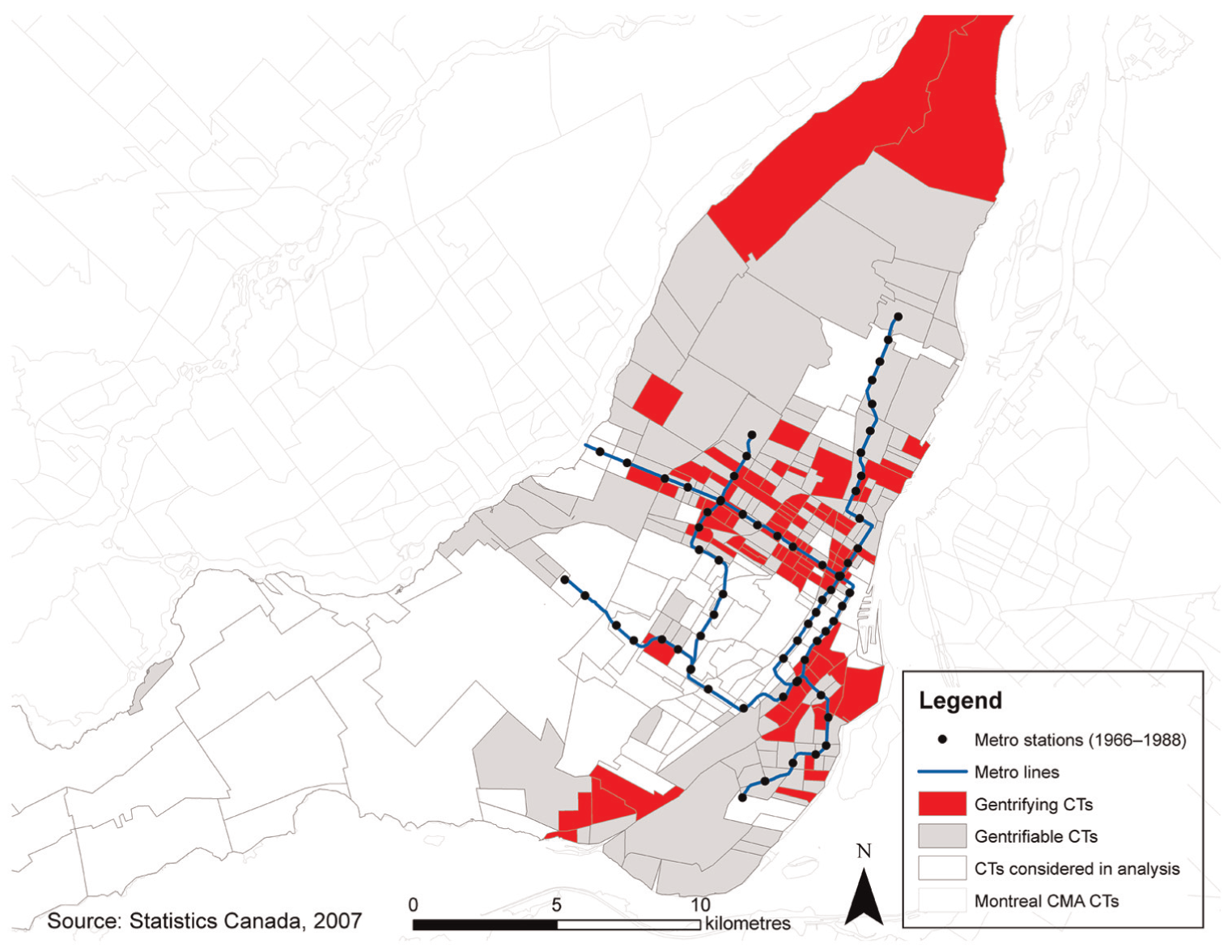
Gentrifiable and gentrifying census tracts in Montreal (1961–2006).

Figure 3.

Gentrifiable and gentrifying census tracts in Vancouver (1986–2006).

Survival analysis

As explained in the literature review, gentrification is conventionally identified by the use of several variables jointly, that all need to increase at a rate faster than the surrounding region over a given period of time. If a particular CT (that is gentrifiable) experiences a relative (to its CMA) increase of all the relevant variables at the same time, it is considered to have undergone gentrification. As we are identifying when a census tract has experienced the onset of gentrification the dependent variable is more appropriately thought of as an event. The most common statistical technique adapted to event analysis is survival analysis.

Primarily used in the field of bio-statistics, survival analysis has had limited use in transportation research, but it is still particularly relevant to the field (Washington et al., 2003). Survival analysis is a collection of statistical procedures for analysing data where the outcome variable is time until an event occurs (Kleinbaum and Klein, 2005). The result of survival analysis is to make statistical inferences about how a given independent variable affects the probability of the event occurring at a given time. This type of analysis is particularly useful when working with variables whose effects vary over time, called time dependent variables (Kleinbaum and Klein, 2005).

Examples of applications of this type of analysis include time until death of patients with or without a certain type of treatment (Kleinbaum and Klein, 2005), or time until an accident occurs after a driver has obtained their licence (Washington et al., 2003). A related approach, ‘spatial hazard analysis’, where duration is substituted with distance as the outcome variable, has more commonly been applied in a planning context. Carruthers et al. (2009) used the approach to analyse urban form and sprawl in American metropolitan areas.

In the model presented in this paper the ‘event’ is gentrification and the ‘treatment’ variable is proximity to stations of rapid rail transit. The population in question is all of the census tracts that are deemed gentrifiable in the previous census period. As such, a census tract enters the sample in the year that it becomes gentrifiable, and leaves when it either experiences gentrification, or when the study period ends, whichever occurs first. Census independent variables (e.g. % pre-1946 housing) change for each census and distance to transit stations was recalculated every time there were stations added to the system in question. The results of the model give the survival time of CTs until they gentrify based on the presence of transit over time, as well as the control variables used in the models.

In initial analyses for this research, we found that there is not a simple linear relationship between gentrification and distance to transit. Instead, it appeared that gentrifying census tract centroids were often close to stations, but less likely to be immediately adjacent. As a result, a gravity function was used to capture the effect of distance from transit to an individual CT, and was calculated for each CT for each year of the study as a function of distance to the nearest station –‘cdist’ in Equation 1 (see De Dios Ortúzar and Willumsen, 2001, for more examples of gravity functions). Alpha and beta are parameters that adjust the height and location (along the horizontal –‘cdist’– axis) of the maximum of the gravity function. Alpha is positive (with a value of 1 used for all cities) and beta is negative, with the value changing for cities depending on what resulted in the highest value of the log likelihood function. The result is a gravity function that at first increases and then decreases along the horizontal axis.

Equation 1: Exposure gravity measure

\exp o = cdis t^{α} * e^{β * cdist}

We refer to this gravity measure of proximity to transit as ‘exposure’. The distance to transit stations, ‘cdist’, was recalculated for each year that new transit stations were added to the transit network. Before being included in the statistical analysis, the variable was normalised to 1 to facilitate comparability of coefficients across cities.

The survival model

The extended Cox (EC) model was selected for the analysis in this study. The rest of this section draws primarily on Kleinbaum and Klein (2005). The EC model is a semi-parametric model and therefore less restrictive in terms of the assumptions made about the form and distribution of the hazard function. Whereas parametric survival models assume that survival time follows a known distribution (e.g. Weibull, exponential, log-logistic, etc.), this assumption is not made in the case of the extended Cox model. This semi-parametric model allows the hazard function, and survival time, more flexibility. In this model the Hazard Ratio is also allowed to change over time. This model also allows for the analysis of time dependent variables, which are present in this model. The two parts of the EC hazard function (see Equation 2) are the baseline hazard function and the exponential function, which incorporates the independent variables in the model.

Equation 2: Extended Cox hazards mode

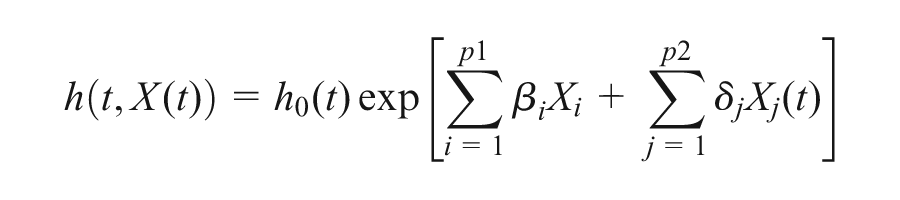
h (t, X (t)) = h_{0} (t) \exp [\sum_{i = 1}^{p 1} β_{i} X_{i} + \sum_{j = 1}^{p 2} δ_{j} X_{j} (t)]

In this equation, X_i represents the time-independent variables and X_j represents the time-dependent variables, denoted by the presence of (t). The coefficients, beta and delta, are estimated using maximum likelihood techniques. The variables included in the models for each of the three cities are outlined in the next section with an interpretation of the results.

Survival model estimation results

Many models and many variables were tested to arrive at the models presented here. Variables tested included the proportion of pre-1946 housing, measured for each census year; the exposure measure; distance to the nearest park; distance to the nearest major body of water; distance to nearest previously gentrifying CT; and distance to the CBD. Different interactions between variables, and between the variables and time, were also tested. The gravity measure, ‘exposure’, was recalibrated for each city as the effect of transit was maximised at a different distance from the transit stations for each urban centre.

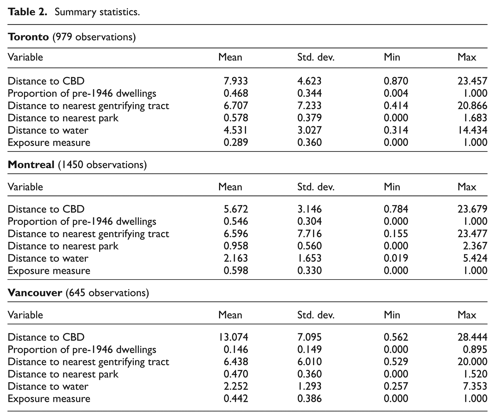
While tempting to include census variables such as income, number of degrees, and so on, as independent variables, they cannot be used since they are used to define gentrification itself and as a result would be endogenous. Table 2 presents summary statistics for the main (not interacted) variables used in model development and estimation.

Table 2.

Summary statistics.

Toronto (979 observations)
Variable	Mean	Std. dev.	Min	Max
Distance to CBD	7.933	4.623	0.870	23.457
Proportion of pre-1946 dwellings	0.468	0.344	0.004	1.000
Distance to nearest gentrifying tract	6.707	7.233	0.414	20.866
Distance to nearest park	0.578	0.379	0.000	1.683
Distance to water	4.531	3.027	0.314	14.434
Exposure measure	0.289	0.360	0.000	1.000
Montreal (1450 observations)
Variable	Mean	Std. dev.	Min	Max
Distance to CBD	5.672	3.146	0.784	23.679
Proportion of pre-1946 dwellings	0.546	0.304	0.000	1.000
Distance to nearest gentrifying tract	6.596	7.716	0.155	23.477
Distance to nearest park	0.958	0.560	0.000	2.367
Distance to water	2.163	1.653	0.019	5.424
Exposure measure	0.598	0.330	0.000	1.000
Vancouver (645 observations)
Variable	Mean	Std. dev.	Min	Max
Distance to CBD	13.074	7.095	0.562	28.444
Proportion of pre-1946 dwellings	0.146	0.149	0.000	0.895
Distance to nearest gentrifying tract	6.438	6.010	0.529	20.000
Distance to nearest park	0.470	0.360	0.000	1.520
Distance to water	2.252	1.293	0.257	7.353
Exposure measure	0.442	0.386	0.000	1.000

Following are the results for the three cities and a brief description of each. The number of subjects is the number of gentrifiable CTs included in the analysis and the number of failures is the number of census tracts that were observed to have experienced gentrification at some point during the study period.

The model describing gentrification in Toronto is presented in Table 3. Since the extended Cox model is fitted using maximum likelihood estimation, the appropriate goodness of fit statistic is the likelihood ratio (LR) test (Blossfeld et al., 2007). This tests the hypothesis that, jointly, the variables in the model have no influence on survival time. The LR statistic is X² distributed with degrees of freedom equal to the number of coefficients estimated. The LR statistic for this model is 35.68 rejecting the null hypothesis of no influence at almost any level significance (STATA reports a p-value of 0.0). With respect to model coefficients, exposure was statistically significant and positive, meaning that as the exposure measure increases there is an associated increase in the likelihood of a CT gentrifying. It is important to understand the meaning of the exposure measure. In the case of Toronto, the maximum of the exposure measure, 1, is found at a distance of 550 metres from a metro station. In order to get the odds multiplier for the variable in this model, we raise e to the power of the coefficient for exposure from the model. This gives an odds multiplier of just over 5, indicating that according to the model, if a subway station is built 550 metres away from a CT which previously had no access to transit, that census tract would be five times more likely to gentrify as a result.

Table 3.

Extended Cox model survival analysis results for Toronto and Montreal.

Toronto results
Variables	Coefficient	Std err	z	P > z
Exposure	1.910	0.7893	2.420	0.016
Proportion of pre-1946 dwellings	1.374	0.4677	2.940	0.003
Proximity to nearest gentrifying CTs	−0.119	0.0310	−3.830	0.000
Exposure*time	−0.0968	0.0050	−2.790	0.005
Descriptive statistics
Initial log likelihood	−339.987
Final log likelihood	−322.147
Observations	979.000
Subjects	163.000
Failures	71.000
Montreal results
Variables	Coefficient	Std err	z	P > z
Exposure	1.276	0.642	1.990	0.047
Exposure*distance to CBD	−1.444	0.664	−2.180	0.030
Proximity to nearest gentrifying CT	−0.133	0.057	−2.320	0.020
(Exposuredistance to CBD)ln of time	0.335	0.199	1.680	0.092
Descriptive statistics
Initial log likelihood	−439.790
Final log likelihood	−422.301
Observations	1453.000
Subjects	220.000
Failures	86.000

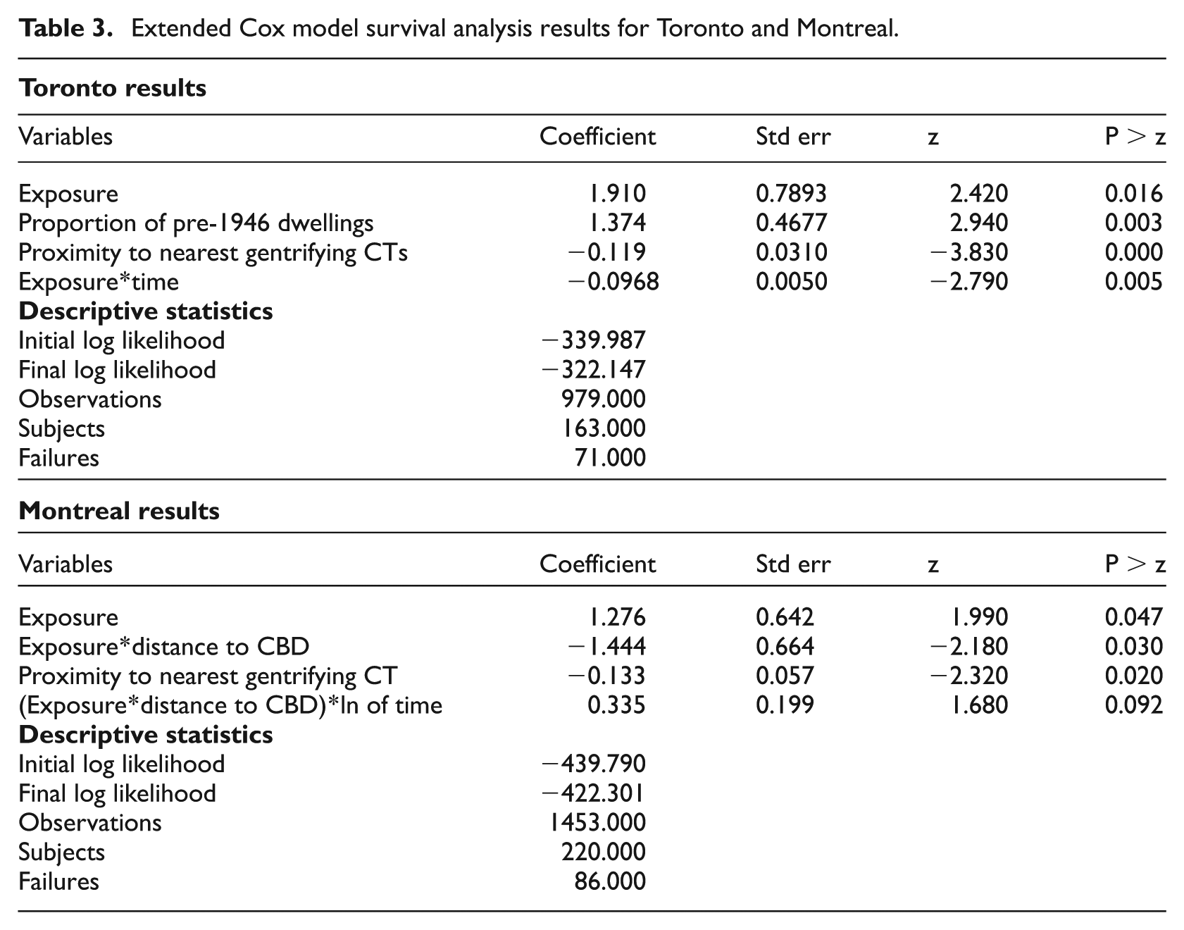
The proportion of housing built before 1946 was also statistically significant, which reinforces findings by others that consider the importance of housing stock (Walks and Maaranen, 2008). Another variable (proximity to nearest gentrifying CT) is included to answer the question of whether the effect of gentrification is one that ‘spreads’. The coefficient of this variable indicates that as the distance to the nearest already gentrifying or gentrified CT increases, the likelihood of gentrification decreases.

The elasticities (estimated at the mean) of each of these main variables are reported to provide a sense of the ‘effect size’ of each of the variables. Their values are: exposure, 0.55; proportion of pre-1946 dwellings, 0.64; and proximity to nearest gentrifying tracts, -0.79. These imply that a 1% increase in the exposure measure results in a 0.55% increase in the hazard ratio; the same proportional increase in pre-1946 dwellings results in a 0.64% increase, whereas a 1% increase in distance to the nearest gentrifying tract results in a 0.79% decrease in the hazard ratio. These elasticities are all in the same order of magnitude with the exposure measure being smaller than the others.

The negative coefficient of the last variable included, an interaction of exposure with time indicates that the effect of exposure on gentrification is greatest soon after transit is implemented and then decreases as time goes on.

As was the case for Toronto, in the results of the Montreal model (see Montreal results in Table 3) the LR test rejects the null hypothesis in the model at almost any level of significance with a value of 34.98 and 4 degrees of freedom. The variables included in the model for Montreal were the Exposure measure, the interaction between exposure and the distance to CBD, and the proximity to nearest gentrifying CT, all of which were found to be significant at or below 5%. An interaction between exposure, distance and the natural logarithm of time was found to be significant at 10%. The positive coefficient of Exposure tells us that a higher exposure value is correlated with a higher likelihood of a CT gentrifying. As distance to the nearest gentrifying CT decreases, the likelihood of a CT gentrifying increases. The elasticities (estimated at the mean) of these main variables are: exposure, 0.76 and proximity to nearest gentrifying tracts, -0.88. These imply that a 1% increase in the exposure measure results in a 0.76% increase in the hazard ratio, whereas a 1% increase in distance to the nearest gentrifying tract results in a 0.88% decrease in the hazard ratio. These elasticities are in the same order of magnitude as in Toronto, and as with Toronto, the exposure measure has a smaller elasticity than distance to the nearest gentrifying tract.

The interacted variable of exposure and distance to the CBD implies that metro stations located further from the CBD initially have less of an effect on gentrification, but as time goes on the distance from the CBD becomes less important, and gentrification is more likely to occur. This appears to be capturing the spreading of gentrification away from the city’s centre over time.

Estimation of a correlation matrix for the main variables tested in both the Toronto and Montreal models, respectively, produced correlations both below |0.7|.

In the case of Vancouver, despite many different models being tested, only one of the variables – distance from water – proved to be statistically significant to the onset of gentrification with a positive coefficient indicating that as distance to water increases, the likelihood of gentrification increases. This may seem surprising to readers familiar with Vancouver since many of the city’s famously gentrified neighbourhoods (e.g. Kitsilano) are found close to the water. At the same time it needs to be highlighted that by 1981 (the first year of the study period), these neighbourhoods are recognised as having already gentrified (Walks and Maaranen, 2008), explaining why they were not identified as gentrifiable, and therefore not included in our analysis.

The lack of correlation between transit and gentrification in Vancouver is consistent with recent findings that demonstrate that poverty is actually spreading along the SkyTrain lines, rather than gentrification as seems to be the case in other cities, such as Toronto (Ley and Lynch, 2012).

To summarise our results, it is worth contrasting them with those of others who have examined the question of transit and gentrification. The results of the three studies described in detail in the literature review demonstrated that transit has had varying effects with regards to gentrification; in some neighbourhoods it seemed related to the process and in others not (Kahn, 2007; Lin, 2002; Pollack et al., 2010). We find that in Montreal and Toronto there is a positive relationship between transit exposure and gentrification, whereas in Vancouver there does not seem to be any effect of exposure to transit. As with Kahn (2007) and Pollack et al. (2010) we find variability in the relationship between transit and gentrification by city. Unlike in the multi-city study conducted by Kahn (2007), where a negative relationship between transit and housing values was observed in some cases, we find no evidence of transit having a negative impact on gentrification in any of the cities examined.

Discussion and conclusions

This paper contributes to literature on gentrification and transit by identifying the process in a manner that is consistent with the broader gentrification literature and applying an appropriate and innovative statistical technique to test its relationship to transit in the three largest Canadian cities. As such, and according to the definition of the onset of gentrification as an event, we argue that an event analysis approach, such as survival analysis, is a more appropriate method than what has been used in past studies.

Our results show statistically significant and positive relationships between exposure to urban rail transit stations and the likelihood that CTs undergo gentrification in Toronto and Montreal, although not in Vancouver. These results are similar to previous research that has found mixed results in terms of the relationship between transit and gentrification, although unlike previous studies, we find no evidence of a negative relationship between the two.

While the approach employed in this paper is more appropriate than methods used in previous studies, the models could certainly be improved. In particular, more precise information on accessibility to tertiary employment, information on commercial districts, and perhaps most importantly, municipal policies and investments associated with the development of the urban environment as these rail systems were built would be informative. The inclusion of these variables in the future would help us to better understand the process of gentrification, and tease out the effect that transit plays. It will also be interesting to watch, as new censuses become available, how gentrification evolves over time in different urban centres as well as expanding the studies to encompass smaller, regionally important urban centres and other forms of transit such as Bus Rapid Transit. The integration of the aforementioned variables and the expanded scope of studies represent important avenues for future research on the topic.

The study of gentrification remains an important and relevant topic in research on the changes occurring in cities worldwide, as it has been observed to have adverse effects, especially on poorer communities. Public investments, such as transit infrastructure, could be contributing to gentrification and therefore the implications of these investments, including those of public transportation, need to be well understood in order to mitigate any harmful effects, which could include rising costs of living for existing residents, conflicts within communities and even displacement. Although not all of the impacts of the implementation of transit may be fully known before it occurs, it is important for planners to include integrated neighbourhood and transportation plans to help provide affordable housing options accessible to transit. If transit is not made accessible to those populations who would receive the greatest marginal benefit from its use, then it is not fulfilling its role of increasing the equity and accessibility of urban spaces.

This study contributes, in an innovative and applicable way, to the burgeoning field of research pertaining to the effects of transit on the process of gentrification. The research presented here should be used to inform planners and researchers about the many effects of the implementation of transit, which may occur as a result of increased accessibility to transit, in order to mitigate the negative effects of gentrification and displacement.

Footnotes

Acknowledgements

We would like to thank the three anonymous reviewers who helped strengthen this article with their comments and corrections.

Funding

This research has been funded through the Canadian Social Sciences and Humanities Research Council (SSHRC) Canada Research Chair’s programme.

References

Atkinson

Bridge

(2005) Introduction. In: Atkinson

Bridge

(eds) Gentrification in a Global Context: The New Urban Colonialism. New York: Routledge, pp. 1–17.

Atkinson-Palombo

(2010) Comparing the capitalisation benefits of light-rail transit and overlay zoning for single-family houses and condos by neighbourhood type in metropolitan Phoenix, Arizona. Urban Studies 47(11): 2409–2426.

Bajic

(1983) The effects of a new subway line on housing prices in metropolitan Toronto. Urban Studies 20(2): 147–158.

Blossfeld

H-P

Golsch

Rohwer

(2007) Event History Analysis with Stata. New York: Psychology Press.

Carruthers

Lewis

Knaap

G-J

. (2010) Coming undone: A spatial hazard analysis of urban form in American metropolitan areas. Journal of Papers in Regional Science 89(1): 65–88.

Cervero

(2004) Effects of light and commuter rail transit on land prices: Experiences in San Diego county. Journal of the Transportation Research Forum 43(1): 121–138.

Clairoux

(2001) Le Métro de Montréal: 35 ans déjà. Montréal: Hurtubise HMH Ltée.

de Dios Ortúzar

Willumsen

(2001) Modelling Transport (3rd ed). Chichester: John Wiley and Sons.

Debrezion

Pels

Rietveld

(2007) The impact of railway stations on residential and commercial property value: A meta-analysis. Journal of Real Estate Economics 35(2): 161–180.

10.

Duncan

(2011) Impacts of transit-oriented development on housing prices in San Diego, CA. Urban Studies 48(1): 101–127.

11.

Filion

(1991) The gentrification – social structure dialectic: A Toronto case study. International Journal of Urban and Regional Research 15(4): 552–574.

12.

Freeman

(2005) Displacement or succession? Residential mobility in gentrifying neighborhoods. Urban Affairs Review 40(4): 463–491.

13.

Hammel

Wyly

(1996) A model for identifying gentrified areas with census data. Urban Geography 17(3): 248–268.

14.

Heidkamp

Lucas

(2006) Finding the gentrification frontier using census data: The cast of Portland, Maine. Urban Geography 27(2): 101–125.

15.

Helms

(2003) Understanding gentrification: An empirical analysis of the determinants of urban housing renovation. Journal of Urban Economics 54(3): 474–498.

16.

Hess

Almeida

(2007) Impact of proximity to light rail rapid transit on station-area property values in Buffalo. Urban Studies 44(5–6): 1041–1068.

17.

Immergluck

(2009) Large redevelopment initiatives, housing values and gentrification: The case of the Atlanta Beltline. Urban Studies 46(8): 1723–1745.

18.

Kahn

(2007) Gentrification trends in new transit-oriented communities: Evidence from 14 cities that expanded and built rail transit systems. Real Estate Economics 35(2): 155–182.

19.

Kleinbaum

Klein

(2005) A Self-Learning Text (2nd ed). New York: Springer.

20.

Kolko

(2007) The determinants of gentrification. Public Policy Institute of California, working paper series. San Francisco: Public Policy Institute of California. Available at: http://papers.ssrn.com/sol3/papers.cfm?abstract_id=985714.

21.

Ley

(1986) Alternative explanations for inner-city gentrification: A Canadian assessment. Annals of the Association of American Geographers 76(4): 521–535.

22.

Ley

Dobson

(2008) Are there limits to gentrification? The contexts of impeded gentrification in Vancouver. Urban Studies 45(12): 2471–2498.

23.

Ley

Lynch

(2012) Divisions and disparities: Socio-spatial income polarization in greater Vancouver, 1970–2005. Research Paper 223. Toronto: University of Toronto Cities Centre. Available at: http://neighborhoodchange.ca/documents/2012/08/summary-version-divisions-and-disparities-socio-spatial-income-polarization-in-greater-vancouver-1970–2005-by-david-ley-nicholas-lynch.pdf (accessed 23 November 2012).

24.

Lin

(2002) Gentrification and transit in northwest Chicago. Journal of the Research Forum in Transportation Quarterly 56(4): 235–263.

25.

Newman

Wyly

(2006) The right to stay put, revisited: Gentrification and resistance to displacement in New York City. Urban Studies 43(23): 23–57.

26.

Metro Vancouver (2010) Local governments of Metro Vancouver. Available at: http://www.metrovancouver.org/about/maps/Maps/Municipalities.pdf (accessed 25 July 2012).

27.

Owens

(2012) Neighborhoods on the rise: A typology of neighborhoods experiencing socioeconomic ascent. City & Community 11(4): 345–369.

28.

Pollack

Bluestone

Billingham

(2010) Demographic change, diversity and displacement in newly transit-rich neighborhoods. Paper presented at the 90th annual meeting of the Transportation Research Board, Washington, DC, 23–27 January 2011. Available at: http://trid.trb.org/view.aspx?id=1093110.

29.

Rose

(2004) Discourses and experiences of social mix in gentrifying neighborhoods: A Montreal case study. Canadian Journal of Urban Research 10(3): 229–245.

30.

Ryan

(1999) Property values and transportation facilities: Finding the transportation-land use connection. Journal of Planning Literature 13(4): 412–427.

31.

Skaburskis

Mok

(2006) Cities as land markets. In: Bunting

Filion

(eds) Canadian Cities in Transition: Local Through Global Perspectives. Toronto: Oxford University Press, pp. 86–101.

32.

Slater

(2004) Municipally managed gentrification in South Parkdale, Toronto. The Canadian Geographer 48(3): 303–325.

33.

Smith

Williams

(1986) Alternatives to orthodoxy: Invitation to a debate. In: Smith

Williams

(eds) Gentrification of the City. London: Allen & Unwin, pp. 1–10.

34.

Statistics Canada (2007) Statistics Canada Census Statistics, 2006. Ottawa: Statistics Canada.

35.

Toronto Transit Commission (TTC) (2012) TTC milestones. Available at: http://www.ttc.ca/About_the_TTC/History/Milestones.jsp (accessed 25 July 2012).

36.

Walks

Maaranen

(2008) The Timing, Patterning and Forms of Community Gentrification and Neighborhood Change in Montreal, Toronto and Vancouver, 1961–2001. Toronto: Center for Urban and Community Studies.

37.

Washington

Karlaftis

Mannering

(2003) Statistical and Econometric Methods for Transportation Data Analysis. Florida: CRC Press.

Supplementary Material

Please find the following supplemental material available below.

For Open Access articles published under a Creative Commons License, all supplemental material carries the same license as the article it is associated with.

For non-Open Access articles published, all supplemental material carries a non-exclusive license, and permission requests for re-use of supplemental material or any part of supplemental material shall be sent directly to the copyright owner as specified in the copyright notice associated with the article.

0.00 MB

0.41 MB

0.40 MB

0.29 MB