Commuting and labour supply revisited

Abstract

According to theory, road pricing may reduce welfare when labour supply is negatively distorted by an income tax. This effect particularly occurs when commuting costs reduce labour supply. We examine the hypothesis that commuting costs reduce labour supply in the short-run. In particular, we estimate the effect of commuting time on labour supply in the UK. We account for endogeneity of commuting time by employing exogenous changes in commuting time resulting from firm relocations and changes in infrastructure. Our results cast doubt on the idea that increases in commuting cost reduce labour supply, at least in the short-run. More precisely, we find that females’ labour supply reacts positively to or is unaffected by increases in commuting time, whereas males’ labour supply is unaffected.

Keywords

commuting time gender labour supply

Introduction

Transport economists have recently become interested in the effect of commuting costs on labour supply. One of the main reasons is that Parry and Bento (2001) argue that a congestion charge may reduce welfare if revenues of this charge are not recycled through income tax reductions.¹ Welfare reductions may occur when labour supply is negatively distorted by an income tax, and is even further reduced by the congestion charge. This result is not in line with the common view that revenue recycling of congestion charges is not essential to obtain efficiency gains (but only useful to obtain political support).

The basic assumption in the paper by Parry and Bento (2001) is that a congestion charge works in a similar way to a reduction in the wage. However, there are reasons to believe that the effect of an increase in monetary commuting costs on labour supply is sometimes quite different from a decrease in net wages. For instance, as we have shown for Germany, an increase in commuting distance reduces the number of days worked, but simultaneously increases the number of hours worked per day (Gutiérrez-i-Puigarnau and Van Ommeren, 2010). As a result, commuting distance slightly increases labour supply. This result differs from the common view that higher commuting costs have a negative effect on labour supply (e.g. Bovenberg and Goulder, 1996; Mayeres and Proost, 2001; Parry and Bento, 2001).

There are a number of important caveats in our previous study and we aim to improve on this in the current paper. First, we use a superior measure of commuting costs, viz. commuting time rather than commuting distance.² Arguably, commuting time is a much better measure than distance in quantifying commuting costs (e.g. Ma and Banister, 2006; White, 1988), because commuting distance is more strongly related to monetary than to time commuting costs, whereas the main cost of travel is due to time losses rather than monetary expenses.³ In the UK, Van Ommeren and Dargay (2006) find that travel costs are mainly associated with time costs. If commuting time rather than monetary commuting costs is what matters in determining labour supply, then by using distance we may strongly underestimate the commute effect.

It is also important to emphasise that economic theory generates different, and sometimes opposite, predictions for the labour supply effects of time and monetary commuting costs. Theoretical models either assume (implicitly) that the number of days worked is freely chosen or that the number of hours per day is freely chosen. When the number of days worked is freely chosen, it can, for example, be shown that monetary commuting costs have a negative effect on the number of days worked (e.g. Calthrop, 2001; Parry and Bento, 2001). However, if the number of hours per day is freely chosen, monetary commuting costs have a positive effect on daily labour supply (e.g. Manning, 2003). Note that both theoretical results are in line with our previous empirical results with commuting distance.

Theory that integrates both types of theoretical model shows that, in general, the effects of both time and monetary commuting costs on labour supply are ambiguous and may even have opposite signs (Fu and Viard, 2012; Gutiérrez-i-Puigarnau and Van Ommeren, 2009). Hence, the reported empirical effect of commuting distance on labour supply is not necessarily informative about the effects of commuting time.

Second, in our previous study, we applied our methodology to Germany. As is well documented, also when compared with many other EU countries, labour supply in Germany is quite restricted because of collective wage bargaining, the presence of unions, etc. So, arguably, our results that labour supply is largely unresponsive may have been explained by the choice of the country.

In the current study we focus on the UK for the years 2004 to 2012. UK labour markets are much more flexible than most other European countries. For example, union practices are less widespread and less restrictive. Furthermore, although the UK is a member of the European Union, many firms do not follow the EU working time directive, which restricts the number of individual working hours to 48 hours per week (Kodz et al., 2001; Neathy and Arrowsmith, 2001). Job durations are shorter than any other EU country, except for Denmark (Mulalic et al., 2013).

One major issue in the empirical study of the effect of commuting time on labour supply is reverse causation. In order to address this issue, we employ an estimation strategy where we focus on the effect of changes in commuting time when these changes are not under the control of the employee because of firm relocations, but also because of changes in congestion or infrastructure, so these changes in commuting time are exogenous for the employee.

It is important to emphasise that exogenous shocks in commuting time occur regularly. In the UK, each year 0.5% of workers state that they change residence because of a firm relocation, implying that firms’ relocations are quite common (Dixon, 2003; National Statistics, 2002). Furthermore, commuting time shocks due to changes in infrastructure are abundant for the period investigated: for example many modifications in motorways (e.g. automatic traffic control on the M42) have reduced commuting times for certain workers, but for other workers commuting time has increased as a result of increases in congestion.

Our study differs from other recent studies that also look at the effect of commuting time on labour supply of teachers for relocating schools (Fu and Viard, 2012; Gershenson, 2013). It is, however, difficult to generalise their results as in both studies changes in monetary costs of the commute are negligible and the focus is on teachers. In addition, the study by Gershenson (2013) focuses on substitute teachers that can change their labour supply on a daily basis, so it is extremely short term. Note that, in theory, workers may receive full compensation for changes in their commute through wage. Wage compensation for higher commuting costs is possible, and absent any shift of these costs to employees (via higher wages) at the margin one would expect some negative effect on labour supply. However, there are reasons to believe that in a thin labour market only a very small part of the commuting costs are recovered by the employee (Mulalic et al., 2013; Van Ommeren and Rietveld, 2005).

Methodology

In estimating the effect of commuting time on labour supply, we use a similar methodology as discussed in detail in Gutiérrez-i-Puigarnau and Van Ommeren (2010). Basically, we estimate an employee’s labour supply model, specified in a linear-in-commuting first-differences specification:

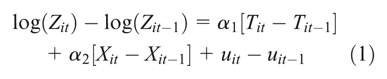
log (Z_{i t}) - log (Z_{i t - 1}) = α_{1} [T_{i t} - T_{i t - 1}] + α_{2} [X_{i t} - X_{i t - 1}] + u_{i t} - u_{i t - 1}

(1)

where the subscript i denotes the employee; subscript t denotes the time period; Z_it denotes weekly working hours; T_it denotes commuting time; the vector X_it includes time-varying controls for household and work characteristics; u_it is the overall error term; and α₁ denotes the effect of the commute on labour supply.

To address possible reverse causation in equation (1) it is important to select the employees who do not voluntary change workplace or residence location. If not, the change in commuting time, T_it − T_it₋₁, may then be related to u_it − u_it₋₁ as a result of the self-chosen employer and residence location.⁴ Although in our data, for reasons of privacy, the exact workplace location is unknown, it is possible to determine whether or not workplace location has not been changed in a certain year, because the data set includes information about changes of employer and changes of type of job. When a certain employee neither changes employer nor type of job, generally this employee does not move into a new job thus endogenously changing the commute. Possible endogeneity issues caused by time-invariant unobserved heterogeneity (e.g. educational level is likely to affect the commute) are as well accounted for in equation (1).⁵

By keeping job type, employer, and residence location constant, any change in commuting time is then the result of (1) an exogenous change in travel speed (e.g. an increase in congestion), (2) an exogenous employer-induced workplace relocation (so the employer moves to another location), or (3) an endogenous change in speed (or measurement error in changes in commuting time).⁶

An endogenous change in speed is possible by changing travel mode. In our analysis, we control for travel mode (and also estimate models on a subsample of employees that do not change travel mode). Changes in congestion or infrastructure that are not under the control of the employee are exogenous to the employee, even if they are known in advance. Most firms announce firm relocations just a few months before they take place, so firm relocations are usually also exogenous shocks. Changes in workplace location (while staying with the same employer) as the firm relocates to another location have been shown to be quite common. Hence, it is extremely plausible that observed changes in commuting time in our data are exogenous when we observe in our data that an employee does not change employer or type of job (and does not change residence), see Angrist et al. (2000).

We can therefore estimate α₁ consistently as the change in commuting time is exogenous (avoiding problems of finding a valid instrument for the endogenous commute). We emphasise that α₁ measures the immediate effect of commuting time, because it is the effect that may occur between the two periods. In our analysis, we focus on a one-year difference. Hence, it is a short-run effect. By focusing on households that do not move residence and workplace, we avoid the problem that in the long-run there may be a selection effect of households who live at their preferred location.

Labour supply analyses

Data

We use the quarterly data from the British Labour Force Surveys (LFS) for the years 2004–2012.⁷ Individuals are observed a maximum of five consecutive quarters. For example, an individual may appear in quarters 1, 2, 3, 4 of 2008 and in quarter 1 of 2009. We select two observations per individual, one year apart (e.g. one observation for an individual in quarter 1 of 2008 and one observation for this individual in quarter 1 of 2009). All other observations are excluded in the analysis. Hence, all workers in our analysis are observed twice, one year apart. We select employed workers aged between 25 and 64, with a positive commute, who work at least two hours per week and maximally 60 hours per week.⁸ We thus disregard self-employees and teleworkers, and those employees whose commuting and weekly labour hours information is missing.⁹

The analysis is further restricted to employees that have one job (95.34% of the employees).¹⁰ We include only observations of employees for which holds that they do not change residence, type of job or employer during the period of observation, which corresponds to 86.40% of the employees. We aim to exclude outliers in changes in commuting time and minimal changes in commuting time. For this reason, we impose that changes in (one-way) commuting time are minimally five minutes and maximally 30 minutes. Observations of changes in commute larger than 30 minutes are extremely rare.¹¹ In contrast, small changes in reported commuting time are extremely common, but are so common that is more likely that they are predominantly due to inaccurate reporting by employees (e.g. the employee reports a commute of 20 minutes and the next year 21 minutes). This type of measurement error causes a downward bias towards zero in the estimate. The analyses are based on a data set of 7664 individuals.

Table 1 shows the summary characteristics of weekly workhours and one-way commuting time, keeping residence location, type of job and employer constant, so for non-movers as well as for movers (who change residence, type of job or employer). The descriptive statistics are almost identical, suggesting that sample selection is not an issue. The mean commuting time for all employees is 27 minutes. It increases by 0.6 minutes per year. More than one-quarter of the employees travel for over 20 minutes. Males commute for 30 minutes compared with 25 minutes for females, emphasising the differences between genders, in line with other studies (e.g. Dargay and Hanly, 2003; Lyons and Chatterjee, 2008; McQuaid and Chen, 2012). In total, employees work about 37 hours per week. Females work on average 32 hours per week, whereas males work about 42 hours, in line with British literature (e.g. Bryan, 2007). The mean change in workhours (in log) for all employees is −0.0079, compared with −0.0067 observed in the overall sample including movers (the median for both samples is 0).

Table 1.

Descriptive statistics of commuting time and weekly labour supply.

	One-way commuting time (min)		Weekly workhours
	Mean	Std. Dev.	Mean	Std. Dev.	N
Males non-movers	30.089	21.063	41.860	7.632	4090
Females non-movers	25.437	18.117	32.304	11.221	3414
Non-movers	27.667	19.683	36.760	10.815	7664
Movers and non-movers	27.013	19.016	36.894	10.649	10,142

Notes: Sample of non-movers refers to employees that (within a period of one year) do not change residence location, nor type of job or employer; sample of movers and non-movers includes employees that change residence location, job or employer; employees hold only one job.

The correlation coefficient between weekly hours (in log) and commuting time is also different for males and females, see Table 2. More importantly, the correlation coefficient between changes in hourly wage and changes in commuting time is essentially zero for the whole sample (0.0235), slightly positive for females (0.0494) and zero for males (−0.0089). This indicates that in the short-run, commuting time has little, or no, effect on labour supply.

Table 2.

Correlations of commuting time and weekly labour supply.

	Commuting time and weekly hours		Changes in commuting time and changes in weekly hours
	Correlation	P-value	Correlation	P-value	N
Males	0.0587	0.0000	−0.0089	0.7085	4090
Females	0.1824	0.0000	0.0450	0.0421	3414
Total	0.1651	0.0000	0.0235	0.1452	7664

Notes: Pearson correlations; one-way commuting time in minutes; weekly hours for employees holding one job is in logarithm.

The data also contains information on full-time versus part-time job, workplace union presence, net monthly earnings, (usual) mode of travel to work, presence of a partner in the household, one-earner versus two-earner household and presence of dependent children. We use as indicator of children the presence of a child younger than 10 years.

Our approach is based on estimating the effect of commuting time on overall labour supply only for the selected group of employees who do not move residence or job when the workplace is relocated or when changes in the commute, such as congestion or infrastructure, are not under the control of the employee (see Angrist et al., 2000). For the group of employees that (within a period of one year) change residence or workplace locations, for example employees that desire to adjust their labour supply may quit and change job (Böheim and Taylor, 2004; Kimball and Shapiro, 2008), the effect of the commute on overall labour supply is not zero. Consequently, we are most likely underestimating the average effect for the whole population.

It seems plausible, however, that the effect we identify holds for the whole UK worker population. After an employer-induced change in the commute or after congestion or infrastructure changes, the employee engages first in a decision process whether or not to relocate and/or change job, and second in a search process to find a residence and/or job that better matches the employee’s preferences on a set of criteria. For the UK, ‘job changes are costly and employment opportunities are not evenly distributed across the hours distribution’ (Böheim and Taylor, 2004: 150). Furthermore, the majority of employees will not move residence within the period of a year, as households face substantial residential moving costs (Weinberg et al., 1981).

The yearly rate of residential mobility of people aged 16–64 in the UK labour force is about 11%; 6.1% of all residential changes are attributed to a job or employer move, 2.4% to a residential move given workplace, and only 0.6% to a workplace relocation (Dixon, 2003). This suggests that only a small fraction of employees will move residence or job within a year, after an employer-induced change in the commute or after congestion or infrastructure changes.

The literature emphasises that gender plays an important role in explaining labour market behaviour as well as travel choices and full-time status (e.g. Crane, 2007). Table 3 shows differences between male and female workhours and commuting patterns by mode shares and by people who work full-time or part-time. For this reason, we focus on the gender-specific effect of the commute on labour supply.

Table 3.

Commuting time and weekly labour supply patterns.

	Weekly workhours				One-way commuting time (minutes)
	Part-time jobs		Full-time jobs		Part-time jobs		Full-time jobs
	Females	Males	Females	Males	Females	Males	Females	Males
	Mean (Std. Dev.)	Mean (Std. Dev.)	Mean (Std. Dev.)	Mean (Std. Dev.)	Mean (Std. Dev.)	Mean (Std. Dev.)	Mean (Std. Dev.)	Mean (Std. Dev.)
Auto commute	22.56 (14.80)	26.59 (17.09)	26.21 (16.46)	27.79 (17.50)	23.76 (7.85)	27.91 (7.66)	41.37 (5.09)	43.47 (5.85)
Bus/metro/tram commute	38.88 (23.27)	52.06 (15.32)	49.27 (18.93)	47.62 (18.31)	25.33 (6.99)	29.66 (7.36)	42.13 (5.81)	44.77 (6.41)
Train commute	55.51 (27.30)	61.33 (18.98)	65.27 (22.70)	66.95 (30.37)	26.02 (7.14)	32.85 (4.54)	41.79 (5.51)	43.94 (5.89)
Walk/bike commute	14.92 (8.58)	16.43 (8.71)	19.47 (12.82)	19.60 (12.74)	20.80 (8.21)	26.92 (7.90)	40.92 (5.19)	42.68 (5.15)
N	1691	429	1723	3661	1691	429	1723	3661

Notes: Employees holding only one job; 35 or more hours per week is considered full-time employee.

Estimation results

The results of several first-differences models based on equation (1) are shown in Table 4.¹² Our result including no controls (except for year dummies) indicates that, ceteris paribus, commuting time has a positive, although insignificant, effect on logarithm of weekly hours, with an estimate of about 0.0003 (s.e. 0.0003), see column [1].

Table 4.

Estimates of logarithm of weekly labour supply (first differences).

	Total						Females					Males
	[1]	[2]	[3]	[4]	[5]	[6]	[7]	[8]	[9]	[10]	[11]	[12]	[13]	[14]	[15]	[16]
Commuting	0.0003	0.0004	0.0005				0.0008	0.0009	0.0012	0.0010		−0.0002	−0.0004	−0.0005	−0.0001
	(0.0003)	(0.0003)	(0.0003)				(0.0004)*	(0.0006)	(0.0005)**	(0.0005)**		(0.0004)	(0.0005)	(0.0004)	(0.0004)
Commuting x female				0.0008	0.0008	0.0009
				(0.0004)*	(0.0004)*	(0.0005)
Commuting x male				−0.0001	−0.0001	−0.0001
				(0.0003)	(0.0004)	(0.0004)
Commuting x child								−0.0002					0.0004
								(0.0008)					(0.0005)
Commuting x two−earners								−0.00001					−0.00002
								(0.0005)					(0.0003)

Commuting x decreases											0.0019					0.0001
											(0.0007)**					(0.0006)
Commuting x increases											−0.0001					−0.0004
											(0.0006)					(0.0004)
Bus/metro/tram commute		−0.0038	−0.0134		−0.0006		−0.0347	−0.0352	−0.0995		−0.0354	0.0252	0.0269	0.0732		0.0252
		(0.0235)	(0.0353)		(0.0233)		(0.0333)	(0.0337)	(0.0355)**		(0.0330)	(0.0324)	(0.0333)	(0.0544)		(0.032)
Train commute		0.0054	0.0255		0.0079		−0.0259	−0.0258	−0.0219		−0.0230	0.0270	0.0243	0.0752		0.0262
		(0.0222)	(0.0286)		(0.0221)		(0.0318)	(0.0317)	(0.0398)		(0.0317)	(0.0286)	(0.0284)	(0.0375)**		(0.0289)
Walk/bike commute		0.0074	−0.0054		0.0083		0.0068	0.0073	−0.0107		0.0054	0.0112	0.0104	0.0050		0.0112
		(0.0159)	(0.0167)		(0.0159)		(0.0257)	(0.0257)	(0.0264)		(0.0255)	(0.0148)	(0.0148)	(0.0174)		(0.0147)
Partner in household		0.0021	0.0620		0.0048	0.0244	0.0334	0.0406	0.0585	0.0392	0.0325	0.0043	0.0069	0.0024	0.0244	0.0053
		(0.0338)	(0.0592)		(0.0338)	(0.0389)	(0.0320)	(0.0330)	(0.0424)	(0.0375)	(0.0314)	(0.0339)	(0.0343)	(0.0412)	(0.0339)	(0.0339)
Partner x female		0.0316	−0.0042		0.0289	0.0152
		(0.0466)	(0.0401)		(0.0465)	(0.0539)
Two–earner household		0.0014	−0.0033		0.0021	−0.0001	0.0030	0.0026	−0.0020	0.0023	0.0007	0.0014	0.0014	−0.0002	0.0012	0.0012
		(0.0073)	(0.0086)		(0.0073)	(0.0072)	(0.0112)	(0.0187)	(0.0130)	(0.01105)	(0.0113)	(0.0078)	(0.0126)	(0.0091)	(0.0078)	(0.0078)
Child		−0.0381	−0.0319		−0.0375	−0.0400	−0.0545	−0.0602	−0.0434	−0.0418	−0.0559	−0.0376	−0.0265	−0.0290	−0.0375	−0.0375
		(0.0173)**	(0.0186)*		(0.0174)**	(0.0166)**	(0.0315)*	(0.0339)*	(0.0382)	(0.0297)	(0.0315) *	(0.0173)**	(0.0280)	(0.0179)	(0.0173) **	(0.0173) **
Child x female		−0.0165	−0.0132		−0.0172	−0.0018
		(0.0358)	(0.0426)		(0.0358)	(0.0338)
Union		0.0122	0.0001		0.0120	0.0141	0.0153	0.0149	−0.0047	0.0153	0.0112	0.0080	0.0089	0.0046	0.0072	0.0072
		(0.0064)*	(0.0077)		(0.0064)*	(0.0064)**	(0.0102)	(0.0102)	(0.0122)	(0.01012)*	(0.0104)	(0.0072)	(0.0072)	(0.0086)	(.0073)	(0.0073)
Net hourly wage (in log)			−0.1234						−0.1111					−0.1451
			(0.0189)**						(0.0244)**					(0.0293)**
Year dummies	included	included	included	included	included	included	included	included	included	included	included	included	included	included	included	included
N	7664	7248	4834	7664	7248	6730	3414	3414	2210	3150	3414	4090	4090	2624	3580	3834
R-squared	0.0004	0.0060	0.0647	0.0013	0.0069	0.0064	0.0082	0.0088	0.0489	0.0070	0.0113	0.0059	0.1170	0.0065	0.0052	0.0063

Notes: One-way commuting time in minutes of employees holding only one job; union refers to presence of a workplace union; the reference category for commute mode is ‘car’; decreases/increases are dummy variables indicating whether the employee’s commuting time decreases/increases within one year. ^**, ^* indicate that estimates are significantly different from zero at the 0.05 and the 0.10 level, respectively. Standard errors are clustered at the individual level.

Since labour supply and travel behaviour is usually thought to be gender specific, we allow the effect to differ between males and females (column [4]). The effect of commuting time on weekly hours for females is equal to 0.0008 (s.e. 0.0004), so positive and significant at the 10% level. The effect is negative but statistically insignificant for males (−0.0001 with an s.e. of 0.0003). So, our main result seems to be mainly driven by the effect of females’ commuting time.

We also experimented with other specifications for commuting time, but the results are very similar to the results using a linear specification of commuting. For example, the elasticity estimate, using a logarithm of commuting time, is 0.0194 (s.e. 0.0096) for females (significant at the 5% level) and −0.0053 (s.e. 0.0069) for males (not significant at the 5% level). These elasticities correspond to a linear effect of 0.0008 and −0.0002 (evaluated at the mean commuting time). Furthermore, we estimated standard cross-section models (OLS) with the above controls as well as time-invariant controls (e.g. gender). This results in an upward bias in the commute estimate: 0.0040 (s.e. 0.0005) for females (significant at 5% level) and 0.0005 (s.e. 0.0003) for males (significant at 10% level).

Including individual time-varying explanatory variables (columns [2] and [5]), as well as estimating separate models for males and females (columns [7] and [12]), does not appear to be essential for the estimated effect of commuting time. Consequently, our results seem robust to the specification chosen. Both one-adult or two-adult households and households with or without children controls facilitate the interpretation of how working hours and commuting times may be interrelated through these type of households schedules and preferences. We now focus on interactions of commuting time with the latter type of households of interest, see columns [8] and [13]. Our main results as reported above still hold. It appears that the negative effect of commuting time for males is mainly due to the negative effect of observations of households without children.

In the above models, we do not control for wage because it is endogenous. This may be problematic when changes in wages and changes in commuting time are strongly correlated. However, it appears that the partial correlation coefficient between changes in hourly wage and changes in commuting time (so controlling for the explanatory variables included in Table 4), is essentially zero for females (0.0358) as well as for males (0.0175). Hence, not surprisingly, including wage gives the same results (columns [3], [9] and [14]). The latter specification, however, likely suffers from spurious negative correlation because measurement error in hours enters both the left and right hand side of equation (1), a problem known since the publication by Borjas (1980). In addition, in our data, we observe net monthly earnings and monthly hours. Because of much missing information about monthly earnings, the sample size when controlling for wage is much smaller than when not controlling for wage.¹³

One may argue that the transport mode (walking, cycling, by car or by public transport), which is included as a control, is highly endogenous as individuals may change transport mode because they change their labour supply and simultaneously change their earnings. This is, however, less of an issue given our data, as 93% of the employees do not change transport mode. Restricting the analysis to observations of employees not changing transport mode from one period to another does not change the estimated results (columns [6], [10] and [15]).

Our results imply that the size of the effect on female labour supply is not negligible. For example, a large increase in commuting time by 30 minutes one-way (so one hour per day) increases weekly working hours by about 2.5%, which corresponds to an increase of 45 minutes per week for a female employee (with an average weekly supply of 32 hours). A positive correlation between commuting time and work duration is in line with literature discussing this relationship (e.g. Aguiléra et al., 2010; Schwanen and Dijst, 2002).

The finding of a more responsive labour supply of females to commuting time than those of males is not surprising, as females are in general more responsive in their labour market behaviour to changes in commuting time than males (Hersch and Stratton, 1994; Singell and Lillydahl, 1986; White, 1986). A Wald-test indicates that the gender difference in effects is significant at the 10% level (when restricting the analysis to observations of employees not changing transport mode).

To see the importance of analysing a sample of constant job type, employer and residential location, we also estimate models including observations of employees with a residential, job or employer move, so the movers and non-movers sample. The size of the female’s commute effect is now 33% larger than the ones discussed above. The male’s commute effect is statistically insignificant. Hence, to obtain non-upward biased short-run effects it is important to select employees that do not move.

Working hours may not respond in the same way to increases and decreases in commuting time. To test for the latter, in a sensitivity analysis, we estimate models where we allow these effects to differ, see columns [11] and [16]. However, the sample size limits us from getting informative estimates with reasonably small standard errors. The earlier estimates of 0.0008 for females and −0.0002 for males are both within the 95% confidence interval of the increases and decreases in commuting time estimates. We find that the effect is only positive and significant (at the 5% level) when the females’ commuting decreases. The females’ increases and decreases in commute estimates are statistically different using a Wald-test (at the 5% level), whereas the equality of the effects for males cannot be rejected. It appears, however, that when we exclude six observations with extreme weekly hours outliers, we obtain the same results, but we now find that there is no statistical difference between the females’ increases and decreases in commute estimates, and the estimate of the increases in time is now higher though insignificant (at the 5% level). When we exclude even more weekly hours outliers (e.g. 26 outliers), we find the same results and the estimate of the increases in time is now positive though insignificant (at the 5% level). It appears, thus, that we cannot reject the idea that weekly hours respond in the same way to increases and decreases in commuting time.

In the current analysis, we focus on changes in labour supply of employees who neither change jobs nor change employer. Such an analysis is particularly useful when employees are free to choose the number of hours worked. However, employees may be constrained by their employer in their labour supply for many reasons. For example, employees in the retail sector may have rigid daily workhours related to opening hours of stores. Ignoring that some employees may not freely choose their labour supply because of employer restrictions, may produce a downward bias in terms of the magnitude estimate of commuting time on labour supply. We emphasise that this does not reverse the sign of the effect.

To obtain more insight about this downward bias, one may write the average effect of commuting time of both restricted and unrestricted employees as $α_{1} = P_{R} β_{R} + (1 - P_{R}) β_{u},$ where P_R denotes the proportion of restricted employees, and β_R and β_U denote the restricted and unrestricted effects. So, $β_{U} = (α_{1} - P_{R} β_{R}) / (1 - P_{R}) .$ When employees who state that they are restricted are completely restricted (so β_R = 0), then $β_{U} = α_{1} / (1 - P_{R}) .$ In our data, at their current wage, 20.5% of the females and 15.5% of males would prefer their workhours to change. Although we believe that such subjective statements are difficult to interpret, it suggests that the large majority of employees are not constrained in their current labour supply, consistent with Böheim and Taylor (2003, 2004) and Bryan (2007). For females, α₁ is 0.0008 and assuming that between 50% and 80% of females are unrestricted, the effect on the unrestricted female’s labour supply is between 0.0010 and 0.0016, so about 0.25% higher than the original estimate.

Conclusions

The question whether commuting costs reduce labour supply is fundamental to transport economists as it affects the conclusion to what extent revenue recycling is key to obtain welfare improvements of road charging. In this paper we revisit this question. In particular, we focus on the short-run effect of changes in commuting time on an endogenous weekly labour supply, when these changes are exogenous for the employee. Keeping job and residence constant, employees cannot influence the level of commuting costs. Hence, commuting changes must be because of exogenous firm relocations, but also because of involuntary changes in congestion resulting from road pricing or improvements in transport infrastructure.

In the current context, we ignore the response margin that employees may reduce commuting costs by changing job or residence. However, given that our focus is on the short-run, the consequences of ignoring movers seem minor as residential and job moves may take time, compared with the benefit of ensuring a causal effect of the commute on the labour supply.

Using UK data, we find that, at least in the short-run, an increase in commuting time does not have a negative effect on labour supply. In contrast, it has a modest positive effect or no effect on females’ labour supply, and essentially no effect on males’ labour supply. These findings reinforce earlier results for Germany (using commuting distance rather than commuting time). Hence, in particular for females, we have now more empirical evidence casting doubt on the idea that increasing commuting costs reduces labour supply in the short-run.

The intuition of our result is that when commute time decreases, the male employee may simply enjoy the benefit (or when it increases, he simply bears the cost). In contrast, our results suggest that the female employee may react to increases in costs by increasing the number of working hours.

Footnotes

Funding

This research received no specific grant from any funding agency in the public, commercial, or not-for-profit sectors.

Notes

References

Aguiléra

Massot

Proulhac

(2010) Exploring the relationship between work and travel behavior on weekdays: An analysis of Paris Region Travel Survey over 20 years. Transportation Research Record2135: 69–77.

Angrist

Grady

Imbens

(2000) The interpretation of instrumental variables estimators in simultaneous equations models with an application to the demand for fish. Review of Economic Studies67: 499–527.

Böheim

Taylor

(2003) Option or obligation? The determinants of labour supply preferences in Britain. The Manchester School71: 113–131.

Böheim

Taylor

(2004) Actual and preferred working hours. British Journal of Industrial Relations42: 149–166.

Borjas

(1980) The relationship between wages and weekly hours of work: The role of division bias. The Journal of Human Resources15: 409–423.

Bovenberg

Goulder

(1996) Optimal environmental taxation in the presence of other taxes: General equilibrium analysis. American Economic Review86: 985–1000.

Bryan

(2007) Free to choose? Differences in the hours determination of constrained and unconstrained workers. Oxford Economic Papers59: 226–252.

Calthrop

(2001) Essays in urban transport economics. Dissertation, Katholieke Universiteit Leuven.

Crane

(2007) Is there a quiet revolution in women’s travel? Revisiting the gender gap in commuting. Journal of the American Planning Association73: 298–316.

10.

Dargay

Hanly

(2003) A Panel Data Exploration of Travel to Work. Mimeo.

11.

Dixon

(2003) Migration within Britain for job reasons. Labour Market Trends111(4): 191–202.

12.

Viard

(2012) Commute Costs and Labor Supply: Evidence from a Satellite Campus. Mimeo.

13.

Gershenson

(2013) The causal effect of commute time on labor supply: Evidence from a natural experiment involving substitute teachers. Transportation Research Part A54: 127–140.

14.

Gibbons

Machin

(2006) Transport and Labour Market Linkages: Empirical Evidence, Implications for Policy and Scope for Further UK Research. Commissioned for the Eddington Study.

15.

Gutiérrez-i-Puigarnau

Van Ommeren

(2009) Labour Supply and Commuting: Implications for Optimal Road Taxes. Tinbergen Discussion Paper, TI 2009–008/3.

16.

Gutiérrez-i-Puigarnau

Van Ommeren

(2010) Labour supply and commuting. Journal of Urban Economics68: 82–89.

17.

Harvey

(1980) On comparing regression models in levels and first differences. International Economic Review21: 707–720.

18.

Hersch

Stratton

(1994) Housework, wages, and the division of housework time for employed spouses. American Economic Review84: 120–125.

19.

Kimball

Shapiro

(2008) Labor Supply: Are the Income and Substitution Effects Both Large or Both Small? NBER Working Paper No. 14208.

20.

Kodz

Lain

Sheppard

. (2001) Working Long Hours: A Review of Literature and Secondary Data Analysis. Employment Relations Research Series 16.

21.

Lyons

Chatterjee

(2008) A human perspective on the daily commute: Costs, benefits and trade-offs. Transport Reviews: A Transnational Transdisciplinary Journal28: 181–198.

22.

McQuaid

Chen

(2012) Commuting times – The role of gender, children and part-time work. Research in Transportation Economics34: 66–73.

23.

K-R

Banister

(2006) Extended excess commuting: A measure of the jobs–housing imbalance in Seoul. Urban Studies43: 2099–2113.

24.

Manning

(2003) The real thin theory: Monopsony in modern labour markets. Labour Economics10: 105–131.

25.

Mayeres

Proost

(2001) Marginal tax reform, externalities and income distribution. Journal of Public Economics79: 343–363.

26.

Mulalic

Van Ommeren

Pilegaard

(2013) Wages and commuting: Quasi-natural experiments’ evidence from firms that relocate. The Economic Journal DOI: 10.1111/ecoj.12074.

27.

National Statistics (2002) Labour Force Survey LFS 2002. Newport: National Statistics.

28.

Neathy

Arrowsmith

(2001) Implementation of the Working Times Regulations. Employment Relations Research Series 11.

29.

Parry

IWH

Bento

(2001) Revenue recycling and the welfare effects of road pricing. Scandinavian Journal of Economics103: 645–671.

30.

Schwanen

Dijst

(2002) Travel-time ratios for visits to the workplace: The relationship between commuting time and work duration. Transportation Research A36: 573–592.

31.

Singell

Lillydahl

(1986) An empirical analysis of the commute to work patterns of male and females in two-earner households. Urban Studies23: 119–129.

32.

Van Ommeren

Dargay

(2006) The optimal choice of commuting speed: Consequences for commuting time, distance and costs. Journal of Transport Economics and Policy40: 279–296.

33.

Van Ommeren

Rietveld

(2005) The commuting time paradox. Journal of Urban Economics58: 437–454.

34.

Van Ommeren

Rietveld

(2007) Commuting and reimbursement of residential location costs. Journal of Transport Economics and Policy41: 51–73.

35.

Weinberg

Friedman

Mayo

(1981) Intraurban residential mobility: The role of transactions costs, market imperfections, and household disequilibrium. Journal of Urban Economics9: 332–348.

36.

White

(1986) Sex differences in urban commuting patterns. The American Economic Review76: 368–372.

37.

White

(1988) Urban commuting journeys are not ‘wasteful’. Journal of Political Economy96: 1097–1110.