The impact of the American Civil War on city growth

Abstract

This paper analyses the persistence of the shock caused by the American Civil War on the relative city size distribution of the USA. Two features make the study of this conflict interesting. First, it took place at an earlier stage of the industrialisation and urbanisation processes than those previously analysed in the related literature. Second, the battles were fought in the open field, not in urban areas. In line with previous results for the Second World War in Japanese and German cities, our findings suggest that the effects of the shock were transitory. Furthermore, some evidence regarding the possible presence of a ‘safe harbour effect’ is reported.

Keywords

American Civil War relative size distribution shock persistence US city growth

Introduction

The analysis of the consequences of an armed conflict can be carried out from military, political, sociological or economic points of view. In this study, a complementary approach is adopted by considering an urban perspective. The present work examines how persistent the effects of the demographic shocks caused by wars on the relative size of cities are in the case of the American Civil War (ACW, 1861–1865).

In the context defined by the urban structure of the USA in the second half of the 19th century, the wartime and post-war relative population growth rates of a sample of cities of both sides (Union and Confederate) have been analysed in order to answer two questions. First, what are the variables that allow us to identify the ACW demographic shock? Second, did the ACW shock cause transitory or permanent effects on relative city size growth?

This paper argues that the effect of the ACW on the relative size of the biggest cities was transitory, so that their long-term growth patterns were not altered by this armed conflict. This result must be understood in a historical context of intense European immigration and of westward internal migration. Moreover, the post-war decades were coincidental with the industrialisation and urbanisation processes of the Northern states.

It is known that the distribution of relative city size exhibits a high degree of persistence. Reinforcing this finding, previous studies show that strong and temporary demographic shocks caused by wars had only transitory effects and, hence, previous population growth rates are recovered in a few years. This is the case of Davis and Weinstein (2002) who, after proposing an empirical framework, analysed the effects of the Allied strategic bombing on Japanese cities during the Second World War. Also in the context of this conflict, and using a very similar approach, Brakman et al. (2004) studied the consequences of the substantial destruction of German cities. They found some weak evidence of a persistent effect for East German cities while, for West German cities and the whole sample, the effect is transitory.

To the best of our knowledge, only these two studies have explicitly dealt with the effects of wars on urban structures. Nevertheless, it should be noted that, although we focus on a strong temporary demographic shock, recent studies have examined the consequences of more frequent violent events but of a lower intensity on cities, especially after 9/11. In this line, Savitch (2008) carried out an exhaustive study of the effects that terrorism has had in 25 major cities throughout the world. This author concludes that cities are able to recover – in terms of employment, investment and tourism – after terrorist attacks. Another important finding of the study is that the periods of recovery differ across cities and depend, on the one hand, on the magnitude and duration of the attacks and, on the other, on the size of the city and its economic and social cohesion. Coaffee (2009) focused on urban design to promote resilience to terrorism and armed conflicts. Related studies have also explored the impact of terrorism on business and employment (Greenbaum et al., 2007), housing markets (Arbel et al., 2010; Hazam and Felsenstein, 2007) and space (Savitch, 2005) as well as the networks of violent Jihadi extremists (Sageman, 2004).

The ACW has distinctive features with respect to the Second World War and the 9/11 and other terrorist attacks that make studying it of interest. First, the ACW was basically a population shock to cities but, unlike the bombings that related works examine, with little impact on their buildings and infrastructures. This fact conditions the variables to include in the empirical analysis in order to identify the shock. This has been done using the number of war widows and surviving soldiers in the 1890 Census, the male population at the beginning of the conflict and its intensity. Second, and related to the previous feature, the battles were fought in the open field, not in urban areas. For this reason, the number of civilian victims was negligible.¹ Third, it took place at an earlier stage of the industrialisation and urbanisation processes, which, as will be seen in the section ‘Discussion and further results’, is an important aspect. Because of all these peculiarities, this conflict is not just another case study in the literature.

Testing for the persistent nature of the ACW shock

The ACW claimed the greatest number of lives in US history in absolute figures and, especially, in relative ones. Of the 4 million that fought, 620,000 died, about 2% of the total population (Davis, 1960). The sacrifice of this war in terms of population² is evident if the absolute and relative number of dead is compared with the number of Americans who lost their lives during the Second World War (405,399; 0.30% of the US population³) or in Vietnam (58,220; 0.03%). All these figures lead us to conclude that the ACW was a strong but temporary, in the sense that it lasted approximately 4 years, demographic shock that inevitably affected US relative city size distribution. This paper is intended to determine whether the effects of this shock were transitory or permanent. Throughout the article we understand the term ‘shock’ as the population change that cities experienced as a consequence of the war, that is to say, the casualties and movement of people caused by the conflict. The empirical model, data sources, variables analysed and estimation method used to answer this question are presented in this section.

The persistence of the temporal demographic shocks caused by wars on the urban structure of a given country can be analysed using the data of city population in absolute terms. However, it seems more appropriate to work with the share of the city population relative to that of the country. As suggested by Gabaix and Ioannides (2004), this type of normalisation is suitable when analysing long-run issues because it is necessary to work with steady-state distributions. Moreover, working with relative city size allows us to reflect more factors than when using absolute rates: a city can grow in absolute terms but not in relative terms, or vice versa.

The empirical model

Our empirical framework is based on Davis and Weinstein (2002). Let $S_{i, t}$ be city i’s share of total population (relative city size) at time $t$ , and $s_{i, t}$ its natural logarithm. Considering that the initial size of each city, Ω_i, is affected by city-specific shocks ε_i,t we have:

s_{i, t} = Ω_{i} + ε_{i, t}

(1)

For a given time horizon k, the persistence of these shocks is modelled as an autoregressive process:

ε_{i, t + k} = ρ ε_{i, t} + ν_{i, t + k}

(2)

Where ρ $\in$ [0,1] is the persistence parameter. The innovation v_i,t is assumed to be an independently and identically distributed error term.

The persistence parameter in equation (2) reflects how much of a temporary shock is dissipated in k periods. If ρ = 1, then all shocks are permanent and relative city size follows a random walk. If ρ $\in$ [0,1), then relative city size is stationary and shocks are transitory. Further, the closer ρ is to zero, the faster shocks dissipate.

To examine the evolution of relative city size, we take a k-period difference of equation (1):

s_{i, t + k} - s_{i, t} = ε_{i, t + k} - ε_{i, t}

(3)

Substituting equation (2) into (3), it is obtained that:

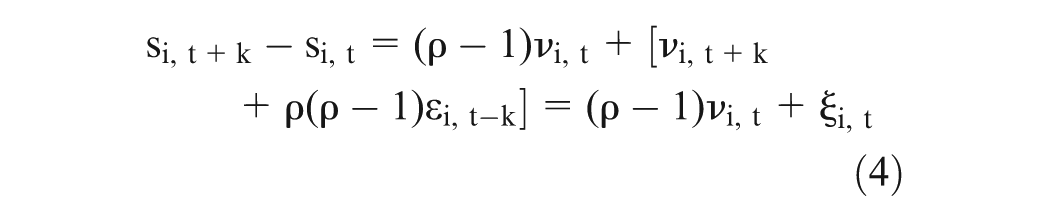
\begin{matrix} s_{i, t + k} - s_{i, t} = (ρ - 1) ν_{i, t} + [ν_{i, t + k} \\ + ρ (ρ - 1) ε_{i, t - k}] = (ρ - 1) ν_{i, t} + ξ_{i, t} \end{matrix}

(4)

As will be further explained in the next subsection, US city population is observed every 10 years (k = 10). Therefore, we are interested in the following version of equation (4) for the relative city size growth rates after the ACW:

s_{i, 1880} - s_{i, 1870} = (ρ - 1) ν_{i, 1870} + ξ_{i, 1870}

(5)

where v_i_,1870 contains the ACW shock and, from equation (4),

ξ_{i, 1870} = ν_{i, 1880} + ρ (ρ - 1) ε_{i, 1860}

(6)

From equation (2), it can be expressed that:

ε_{i, 1860} = ρ ε_{i, 1850} + ν_{i, 1860}

(7)

Combining equations (2) and (3), and referring to the ACW period, leads to:

\begin{matrix} s_{i, 1870} - s_{i, 1860} = ε_{i, 1870 -} ε_{i, 1860} = ν_{i, 1870} \\ + (ρ - 1) ε_{i, 1860} \end{matrix}

(8)

Equation (8) reflects that the shock caused by the ACW is incorporated into the relative city size growth rate during the conflict (s_i_{,1870 −}s_i_,1860). Nevertheless, this growth rate might also contain past information (ε_i,1860) and, given equation (7), will be correlated with equation (6). Therefore, there is a measurement error problem that is further complicated by the data frequency implying that the ACW relative city size shock (v_i_,1870) can only be proxied by the growth rate experienced during the 1860s. These circumstances make it necessary to resort to the use of Instrumental Variables (IV) estimation methods in order to identify the ACW shock and, hence, obtain an unbiased estimation of the persistence parameter.

Summarising, an unbiased estimation of the persistence parameter will be obtained by the application of an IV estimator to:⁴

s_{i, 1880} - s_{i, 1870} = α + β (s_{i, 1870} - s_{i, 1860}) + u_{i}

(9)

where β = (ρ−1) .

The instruments that will allow us to identify the ACW shock must be correlated with the shock but not with the error term in equation (9), which, following equation (6), is given by:

u_{i} = ν_{i, 1880} + (ρ - 1) ε_{i, 1860} + m_{i}

(10)

where $m_{i}$ is related to the measurement error due to the frequency with which the data population is observed.

Data sources and variables

Davis and Weinstein (2002) used deaths and buildings destroyed per capita as instruments for measuring the Second World War shock. Similarly, Brakman et al. (2004) considered the loss of housing stock during this war and its casualties. They also included the amount of rubble in cubic metres per capita as an instrument. As has already been noted, the ACW was basically fought in the open field. For this reason, a measure of the destruction suffered by a city would not be a good instrument to identify the shock.

Blattman and Miguel (2010) pointed out that ‘a major goal of civil war researchers within both economics and political science in the coming years should be the collection of more data’. This is not an easy task for war periods and is even more complicated for conflicts that took place in the 19th century. Taking this into account, the main instrument used in our analysis to identify the ACW demographic shock is the share of war widows as a percentage of the city population. The data were made available for the first time in the 11th Census in 1890, which provided city-level data on ACW widows and veterans, but only for cities that had more than 25,000 inhabitants.⁵ This fact determines the composition of our final sample that consists of data on 104 cities, 93 of them in Union states and 11 in Confederate states. The total US and city population data studied in this paper have been extracted from the Bureau of the Census (Department of the Interior). As noted before, this information is collected every 10 years.

The reason for considering the number of widows in relative terms is to better gauge the intensity of the shock. This variable is expected to be positively related to the shock and negatively to the relative size growth rate during the ACW. This intuition is corroborated by the scatter plot (a) in Figure 1. The 11th Census also reports the number of surviving soldiers by their city of residence in 1890. The converse arguments to those of widows apply to this latter variable: a higher percentage of surviving soldiers is expected to be related to a smaller ACW population shock and to higher relative size growth rates during the war.

Figure 1.

Scatter plot between relative city size growth rate during the 1860s and the percentage of (a) widows and (b) men in the city population.

The shock caused by the ACW is also expected to be related to the number of men from a given city involved in the conflict. In order to reflect this effect, it would be useful to use the number of men of military age (between 18 and 45 years) as an additional instrument, but this information is only available for states. Nonetheless, information is available in the Census about the number of men in a given city, so the proportion of men as a percentage of the total population in 1860 has also been included as an instrument. Although there is no expected sign for the relationship of this variable with the shock, especially if it is introduced as an instrument jointly with the percentage of widows, the scatter plot (b) in Figure 1 suggests that it is positively correlated to the relative size growth rate experienced in the 1860s. This implies that cities with a higher percentage of males at the beginning of the war were less adversely affected by its demographic shock. That is, the higher this percentage, the higher the potential growth resulting from reproductive and labour force motives and, hence, the ACW shock should be less severe.

Another variable that has been used as an instrument is a ‘No Battle’ dummy. According to the US Department of the Interior, there were some 10,500 armed conflicts during the war years, 384 of which can be classified as battles. As a result, this variable takes the value 1 in cities located in states in which none of these battles occurred, and 0 otherwise. Further reasons for the inclusion of this variable, related to the possible presence of a ‘safe harbour effect’, are given in subsection ‘Despcriptive analysis’.

Results

Descriptive analysis

Before estimating the persistence of the ACW shock on relative city size, this subsection describes the demographic trends in the US and the cities that comprise our sample during the period 1850–1890.

The free and slave population, omitting the Indian tribes, increased by 8,251,445 people from 1850 to 1860, a growth rate of 35.46%, which is almost the same as in the previous decade (35.87%). None of the states experienced a decrease in its population until 1860, and New York and Pennsylvania were the most populated states. At the beginning of the war, the population structure was predominantly rural, especially in the Southern states. As an illustration, although New York was the biggest city in the country in 1860, it represented only 20.76% of the state as a whole. In summary, only 13.61% of the population of the USA lived in cities of more than 10,000 inhabitants.

The US population in 1860 was 31 million inhabitants and, contrary to what would have happened if pre-war trends had continued, the figure of 40 million inhabitants still had not been reached by 1870. In fact, the US population growth rate in the 1860s was only 22.62%, a fall with respect to the previous decades. So, it is necessary to analyse the impact of the ACW and, thereby, account for the loss of nearly two million inhabitants, the difference between the population that would have been expected following the pre-war trends and the figure that actually appeared in the 1870 Census.

The deceleration of population growth was not only due to lives lost in the war but also to indirect losses such as those derived from the large number of single men fighting in the war who could not form families, the paralysis of the immigration process and changes in the daily habits of citizens. Nevertheless, the population grew by more than seven million in this decade. Unlike what has been reported for Japan and Germany during the Second World War, all except one city in our sample increased their population in absolute terms during the 1860s.⁶ However, this increase tended to be lower than that of the 1850s. For example, the population of New York increased by 290,111 inhabitants in the 1850s and by 136,634 in the 1860s. Therefore, it can be stated that the ACW led to a slowdown in population growth.

Table 1 reports the growth rates of the USA and the average growth rates of the cities in our sample for the four decades between 1850 and 1890. While, the total population growth decreased in the 1860s with respect to the 1850s, it later recovered in the 1870s, though without reaching its initial level. Nonetheless, the cities that comprise our sample followed a different pattern to that of the country as a whole. On the one hand, it can be observed in the second row that the average growth rate follows a decreasing trend. On the other, the magnitude of the growth rate of the sample cities is higher than that of the country. Further, we have grouped the cities according to whether they are located in a state where battles were fought (third row) or in a state without battles (sixth row). Comparing the two cases, it is observed that, although the average growth rates of both types of cities followed a decreasing trend, the reduction experienced by those in battle zones is nearly negligible between the 1850s and the 1860s. Moreover, if we differentiate the cities in states where more than 15 battles took place (intense) and those with fewer than that number (less intense), it is observed that the former not only did not reduce their growth rate, but experienced a much higher average growth rate during the 1860s.

Table 1.

Population growth rate (%) comparison, 1850–1890.

	1850s	1860s	1870s	1880s
Total USA	35.46	22.62	30.07	24.85
Sample cities	107.49	94.75	55.62	59.64
Battle	105.13	103.30	61.21	61.42
Intense^a	75.68	115.02	31.40	59.20
Less intense^b	115.93	99.28	71.44	62.18
No battle	109.39	87.70	51.00	58.17

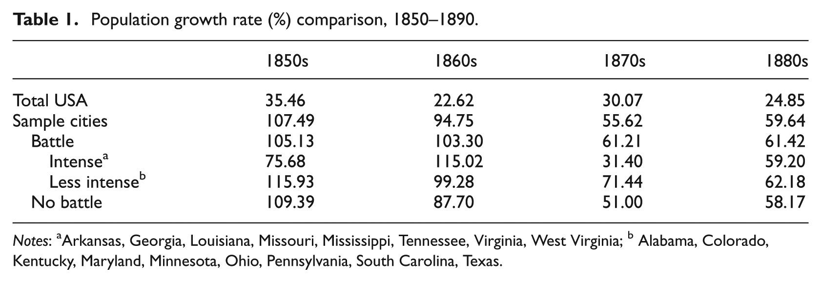
Notes: ^aArkansas, Georgia, Louisiana, Missouri, Mississippi, Tennessee, Virginia, West Virginia; ^b Alabama, Colorado, Kentucky, Maryland, Minnesota, Ohio, Pennsylvania, South Carolina, Texas.

All these figures lead us to suspect that, given the open field character of this war, the big cities might have experienced a ‘safe harbour effect’. As noted by Glaeser and Shapiro (2002):

[T]he first, and probably most important, interaction between warfare and urban development is that historically cities have provided protection against land-based attackers. Cities have the dual advantages of large numbers and walls and thus, holding the size of the attack constant, it is much better to be in a city than alone in the hinterland.

This suspicion will find some support in the subsection devoted to presenting the estimation results.

Testing for instrument validity

The validity of the instruments has been analysed through the application of the Sargan (1958) test of over-identifying restrictions. Its null hypothesis is instrument validity in the sense that they are not correlated with the error term in (IV estimation equation). Given the different combinations of instruments that could be considered, the upper panel of Table 2 reports the test statistics calculated for all the possible pairwise combinations. The null hypothesis cannot be rejected at the 5% significance level in any of the six cases considered.

Table 2.

Statistical tests for instrument validity.

Panel A. Sargan (1958) test
	Survivors	Men	No battle
Widows	3.07	1.80	1.09
	(0.08)	(0.18)	(0.30)
Survivors		0.31	2.66
		(0.58)	(0.10)
Men			2.21
			(0.14)
Panel B. Cragg-Donald (1993) test
	Survivors	Men	No battle
Widows	11.68	5.37	8.19
	(10%)	(25%)	(20%)
Survivors		1.90	1.11
		(25%)	(25%)
Men			2.34
			(25%)

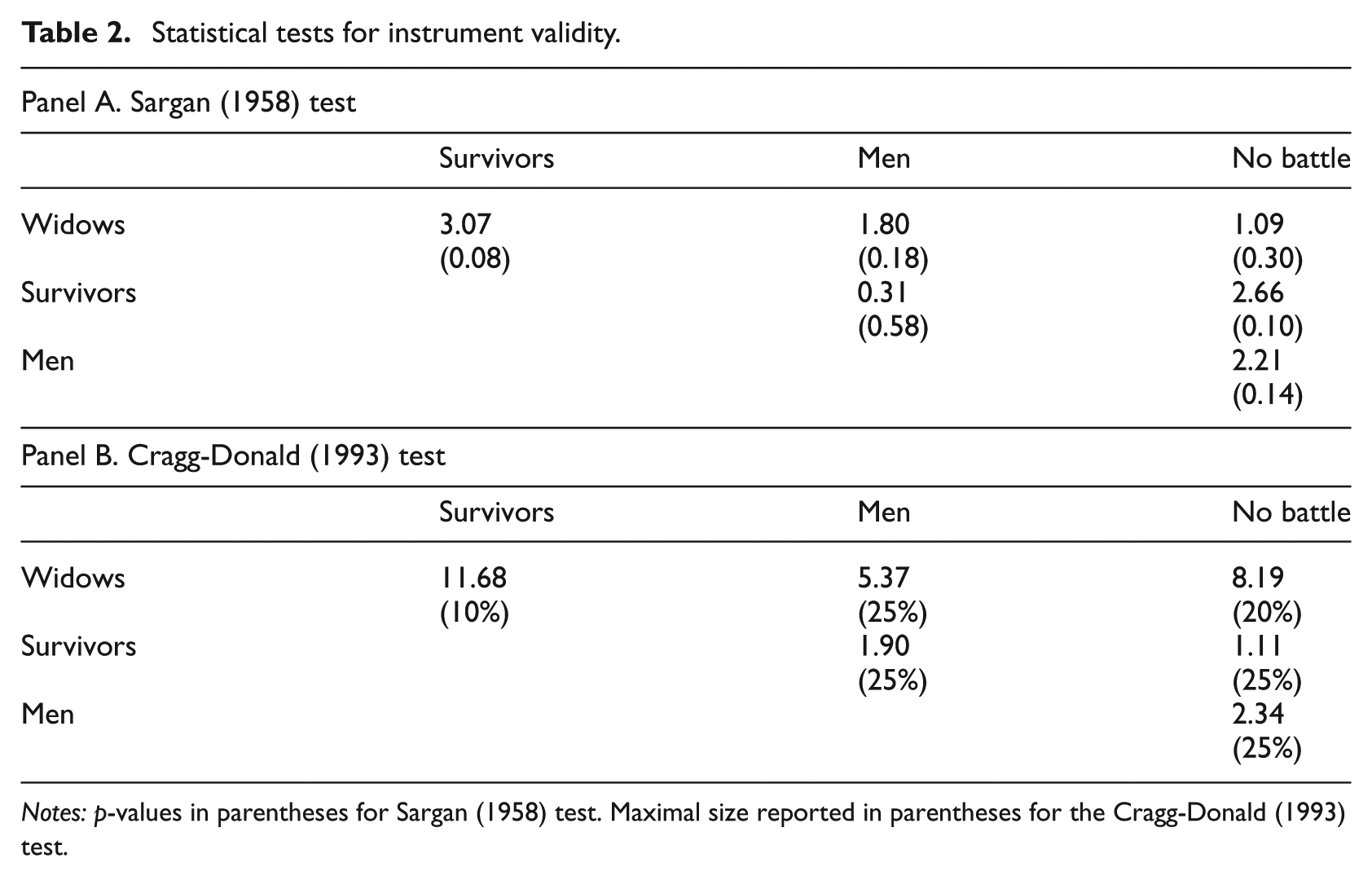
Notes: p-values in parentheses for Sargan (1958) test. Maximal size reported in parentheses for the Cragg-Donald (1993) test.

Following Murray (2006), not only is it important to use instruments that are not correlated with the error term, but they should also be correlated with the instrumented variable. The possibility of a ‘weak instruments’ problem has been analysed by the Cragg and Donald (1993) test, together with the critical values in Stock and Yogo (2005). Results are shown in the lower panel of Table 2 which suggest that the instruments are weakly correlated with the variable being instrumented. Therefore, both the estimated parameters and the inferences using Two-Stage Least Squares (2SLS) will not be reliable (Rothenberg, 1984; Stock et al., 2002). For this reason, the estimation will be carried out using the modification of the Full Information Maximum Likelihood (FIML) method of Fuller (1977). This method has an analytical formulation and a better performance in the presence of ‘weak instruments’ for finite samples.

Estimation of the persistence parameter

Preliminary estimation results⁷ lead us to values of the persistence parameter (1.84–2.18) far from the interval in which it would have economic sense. This finding can be interpreted as evidence of the presence of some distorting influence. Given the type of data we are working with, the low determination coefficients obtained in the first stage estimations of the exploratory analysis, and the scatter plots in Figure 1, our suspicion is that these estimations are biased by some outlying observations (Dehon et al., 2009a; Wagenvoort and Waldmann, 2002).

To confirm this intuition, for the first stage estimation, we have used the graphical tool for outlier detection of Rousseeuw and Van Zomeren (1990), based on the application of robust statistics. The results are plotted in Figure 2. Following the classification in Rousseeuw and Leroy (1987), three cities can be considered as especially ‘bad leverage points’: Omaha (Nebraska), Kansas City (Missouri) and Denver (Colorado). The presence of this type of outlying observation significantly affects estimated parameters which, in the end, will lead to a biased estimation in the second stage.

Figure 2.

Outliers in the first stage of the IV estimation. Cities in the grey areas can be considered as bad leverage points that may lead to biased estimations. The other cities are good leverage points whose presence only affects the magnitude of the standard errors.

This graphical impression is confirmed by the Hausman-type test to detect the presence of influential outliers in regression analysis proposed by Dehon et al. (2009b). When it is applied to the first stage regression, the null hypothesis of no contamination can be statistically rejected at the 5% significance level. However, when these three outlying cities are dropped, the corresponding p-value is 0.58, which is almost the same as that obtained when using a dummy variable treatment for these abnormal observations (0.55). Given our reduced sample size, we have chosen to apply the latter approach in order to control for the possible bias.

FIML estimation results are reported in Table 3. The upper panel shows those corresponding to the first stage when the relative city size growth rate during the 1860s is regressed on the instruments. The second and third columns give the results obtained for our first specification when three instruments are used to identify the shock: widows as a percentage of the population in 1890, the share of men in 1860 and the ‘No battle’ dummy. The signs of the estimated parameters are the expected ones and the three instruments are statistically significant. This is also the case for the three dummies that control for the presence of the outlying observations.⁸ Furthermore, the goodness of fit is reasonable, the coefficient of determination being 0.46. The results for the second stage can be seen in the lower panel of Table 3. The estimated value for the slope parameter (β) in (IV estimation equation) is −0.60, which corresponds to an estimated persistence parameter (ρ) of 0.40. This leads us to conclude that the nature of the demographic shock derived from the ACW on relative city size growth was transitory.

Table 3.

Full Information Maximum Likelihood (FIML) estimation results.

Specification
	(1)			(2)
Panel A. First stage
Endogenous variable: Relative city size growth 1860–1870 (g_i_,60-70)
	Coefficient		SE	Coefficient		SE
Constant	−0.82*		0.46	−0.78*		0.44
Widows	−0.69***		0.20	−1.44***		0.29
Survivors				0.22***		0.07
Men	0.03***		0.01	0.03***		0.01
No battle	−0.20**		0.07	−0.16**		0.07
R ²		0.46			0.52
Observations		104			104
Panel B. Second stage
Endogenous variable: Relative city size growth 1870–1880 (g_i_,70-80)
	Coefficient		SE	Coefficient		SE
Constant	0.34***		0.12	0.27***		0.09
g_i _,60-70	−0.60*		0.32	−0.40***		0.24
Persistence ( $\hat{ρ}$ )		0.40			0.60

Notes: The modification proposed by Fuller (1977) of the FIML estimation method has been implemented. First stage estimations include dummy variables for Omaha, Kansas City and Denver. ***, ** and * denote statistically significant at the 1, 5 and 10% level, respectively.

The fourth and fifth columns of Table 3 show the estimation results when the surviving soldiers as a percentage of the total population of the city in 1890 is also included as an instrument. Our results suggest that this variable is positively related to the growth rate during the 1860s and is statistically significant. Moreover, its inclusion does not affect either the sign of the rest of instruments or their statistical significance while, at the same time, the coefficient of determination increases (0.52). The main consequence of including this additional instrument is that the estimation of the persistence parameter increases to 0.60. This implies that, although transitory, the persistence of the shock is higher.

In sum, the analysis carried out in this section allows us to reach two conclusions. First, the shock caused by the war on relative city size was greater, (1) the higher the percentage of widows of soldiers who died in the ACW in the population of the city, (2) the lower the percentage of surviving soldiers in the population of the city, (3) the lower the relative number of males in the city at the beginning of the conflict and (4) the further away the city in question was from the bellic episodes. The latter may be related to the possible existence of a ‘safe harbour effect’. Second, from the estimated value of the persistence parameter, it can be deduced that the shock caused by the ACW on city structure was transitory, which is in line with previous papers that analysed the effects of the Second World War.

Discussion and further results

Economic historians have not been able to reach a consensus about the meaning and the consequences of the ACW in the development and construction of the modern USA. The predominant idea into the 1960s was the Beard-Hacker Thesis (Beard and Beard, 1927; Hacker, 1940) according to which the conflict stimulated the industrialisation and economic growth of the country. Later, authors such as Cochran (1961) and Engerman (1966) questioned this approach, arguing that its effects were not so positive and, in fact, led to a deceleration in development.

Nevertheless, the consensus about the different consequences of the conflict on the economic structure of the two sides is now clear. While the war led to a strengthening and confirmation of the previous means of production in the Union, for the Confederate states it meant the total breakdown of the economic system in force until then. So, apart from slavery, what is it that makes the North so different from the South that the war defines different economic paths?

First, the states of the Union were much more urbanised. Following the figures provided by Ransom (2001), 211 of the 292 counties with an urban⁹ population were in the Northeast and Western regions, representing 78.91% of all urban population in the USA. Moreover, it can also be observed that less than 7% of the population in the Southern states lived in counties that had an urban population. They represented around 10% of the total US population.

Second, while the North was already much more industrial in 1860, the economy of the South was based on agriculture, especially on the cultivation of cotton. These differences with respect to the weight of industry are accentuated after the war. It is well known that the industrial belt of the USA – the Rust Belt – was formed in the last decades of the 19th century in the states that belonged to the Union. According to Frey (1990), this is the region stretching from Maine to Maryland, Ohio to Nebraska, and Minnesota to Kansas. By 1890, the Rust Belt was being consolidated and, according to the data in the Census, accounted for 87.67% of the total manufacturing production of the country.

Third, the evolution of the two economies after the ACW was completely different. Consumption in the North recovered its pre-war level around 1873, while that of the South stayed below its 1860 level until the end of the century (Ransom, 1998). The reason for these differences was their different productive structures. In 1860, 38% of the total population of the 11 Southern states were slaves and the fraction of earnings due to slavery was 26% (Gunderson, 1974). As a consequence of the war, the disappearance of this system of production meant that the South had to ‘reinvent’ its economy. In the meantime, the North underwent a cycle of urbanisation, industrialisation and economic growth. In the words of Ransom (2001): ‘the South was locked in a cycle of poverty that lasted well into the twentieth century’.

Finally, migrations in the late 19th century also affected city populations. It involved not only American ‘pull’ factors (increasing industry and jobs, abundant natural resources and the formation of a stable country) but also European ‘push’ factors (the great potato famine in Ireland, unification and continuous warfare in Germany and congestion in Britain¹⁰).

All the ideas put forward so far in this section lead us to the following important reflection. Bearing in mind that our war period is from 1860 to 1870 and that our post-war period runs from 1870 to 1880, and given the evident predominance of Northern cities in our data, it is possible that what we are characterising as a war shock is a consequence of the overlapping in time of four different phenomena: first, the war and the post-war; second, the urbanisation of the North; third, the formation of the industrial Rust Belt in a large part of the states of the Union; and fourth, immigration from Europe and westward migration. Therefore, we are faced with an identification problem. In other words, to be sure of the character of the war shock, it is necessary to control, as well as possible, given the scarcity of the data available, the other three contemporary phenomena. This has been done through the introduction of variables that refer to these processes (urbanisation, industrialisation and immigration) into the empirical model.

We have included a dummy for the cities in the sample that are located in the Rust Belt, trying to control for the different behaviour of the industrial zone. This variable is not significant and the results, in terms of the parameter of persistence, do not change. We have also included a dummy for the cities in the sample that stayed on the list of the 100 biggest in the USA between 1860 and 1970. This dummy was intended to capture the effect of a prolonged urbanisation. As in the case of the previous dummy, this one is not significant and the results in terms of the parameter of persistence, continue to provide evidence of the transitory character of the ACW shock.

The influence of migratory movements has also been controlled for. The ports of New York, Boston, Philadelphia, Baltimore and New Orleans received more than 90% of all the migrants entering the USA. Therefore, European ‘push’ factors have been proxied by the inclusion of a dummy variable for these cities. Our results suggest that this variable does not explain post-war relative city size growth. In addition, the estimated persistence parameter does not significantly change with the inclusion of this variable. We have tried to control for the American ‘pull’ factors by including an indicator variable for the cities in Western states. Its corresponding estimated parameter is positive and statistically significant. That is, cities in the West tended to experience higher growth after the ACW. Furthermore, the estimated parameter of persistence increases to 0.61. It is worth noting that the inclusion of this variable does not make those that control for the presence of outliers lose their statistical significance. Hence, their atypical character is maintained even after controlling for westward migration.

It can be seen in Table 3 that, when all the processes – war, industrialisation, urbanisation, immigration from Europe and westward migration – are determined simultaneously, $\hat{ρ}$ is 0.4 or 0.6. When trying to control for the four non-bellic processes, as we do in this section, $\hat{ρ}$ is 0.43, 0.41, 0.44 and 0.61, respectively. Consequently, it can be concluded that the effects of industrialisation, urbanisation, immigration and the movement of population towards the West do not essentially alter the persistence/transitory character of the ACW shock.

Concluding remarks

Previous studies have established that German and Japanese cities recovered their pre-Second World War relative size growth rates in a short time. That is to say, the strategic bombing of the Allied air forces during that war only had transitory effects. The only existing evidence of a persistent nature of the shock is weak and corresponds to the cities in East Germany, which is probably related to the change from a market-based to a centrally planned economic system (Brakman et al., 2004).

This paper tries to contribute to the scarce literature about the persistence of the demographic shocks caused by wars on urban structures by analysing relative US city data during the period 1850–1890. The shock derived from the American Civil War (ACW, 1861–1865) is of an important magnitude as more than 600,000 men of the 31 million inhabitants died in the conflict. This figure, especially in relative terms, is much greater than the US lives lost in the Second World War or in Vietnam.

The main conclusion we can draw is that the shock of the ACW also had a transitory effect on relative city size distribution. In addition, evidence has been reported regarding the fact that the US total population growth rate only decelerated in the 1860s with respect to the adjacent decades. Apart from the different historical stage, there are other differences between the ACW and the Second World War. While the latter caused many civilian casualties and significant destruction of buildings in Japanese and German cities, the rural nature of the ACW might have led to the appearance of a ‘safe harbour effect’.¹¹

Although, both in this paper and in those of Davis and Weinstein (2002) and Brakman et al. (2004), the effects of wars are found to be transitory, which is notable evidence of cities’ powers of recuperation, the degree of the persistence of the shock is not the same. Davis and Weinstein (2002) find that the estimated parameter of persistence is practically zero for Japan in the Second World War, while Brakman et al. (2004) obtain a value of 0.6 for Germany, also in the Second World War. These results are similar to those obtained in our estimations where we find a level of shock persistence between 0.40 and 0.60, greater than that in Davis and Weinstein (2002) (more persistence) and similar to that in Brakman et al. (2004).

We want to conclude the paper with a further reflection on one of the main results of this work, namely, that the ACW had a transitory effect on city growth. There is a certain consensus that the population and hierarchical structure of cities are very stable over time (Beeson et al., 2001; Black and Henderson, 1999; Eaton and Eckstein, 1997; Kim, 2000) and they are resistant to terrorism and war shocks. Therefore, the consequences of these armed conflicts are not permanent, and cities recover their past growth trends in a few years. This is the result we have deduced for the ACW, in line with the related literature.

Explanations for the stability and resilience of urban structures are based on three arguments: locational fundamentals, which determine where the cities emerge (first nature arguments), reinforced over time by increasing returns and cumulative effects of past investments (second nature arguments). Although it is not easy to alter this stability, this does not necessarily mean that it is the only possible outcome. For instance, locational fundamentals can be eroded by technological change, political events or historical accidents (Polèse and Denis-Jacob, 2010).

Moreover, stability depends on the time period analysed. Like the present study, none of the four papers cited above analyses data over a period longer than 150 years, which can be considered a ‘relatively short’ horizon. In this context, Batty (2006) argues that changes in the internal hierarchy of cities can be important in the very long run. Finally, locational fundamentals are also country-specific, so the same shock can provoke different effects in different countries and urban hierarchies are more volatile in developing nations than in mature urban systems.

Footnotes

Acknowledgements

The authors have benefited from the helpful comments of three anonymous referees and those of Domingo Pérez, Vicente Pinilla and Mario Polèse.

Funding

Financial support from Ministerio de Ciencia e Innovación (Project ECO2009-09332), Ministerio de Educación (Grant AP2008-03561) and Gobierno de Aragón (ADETRE research group) is gratefully acknowledged.

Notes

References

Arbel

Ben-Shahar

Gabriel

. (2010) The local cost of terror: Effects of the second Palestinian Intifada on Jerusalem house prices. Regional Science and Urban Economics40(6): 415–426.

Batty

(2006) Rank clocks. Nature 444: 592–596.

Beard

(1927) The Rise of American Civilization. Volumes I and II. New York: Macmillan.

Beeson

DeJong

Troesken

(2001) Population growth in U.S. counties, 1840–1990. Regional Science and Urban Economics31(6): 669–699.

Black

Henderson

(1999) Spatial evolution of population and industry in the United States. American Economic Review89(2): 321–327.

Blattman

Miguel

(2010) Civil war. Journal of Economic Literature48(1): 3–57.

Brakman

Garretsen

Schramn

(2004) The strategic bombing of German cities during World War II and its impact on city growth. Journal of Economic Geography4: 201–218.

Carter

Cartner

Hainer

. (2006) Historical Statistics of the United States: Earliest Times to the Present. New York: Cambridge University Press.

Coaffee

(2009) Terrorism, Risk and the Global City: Towards Urban Resilience. Farnham: Ashgate Publishing, Ltd.

10.

Cochran

(1961) Did the Civil War retard industrialization?Mississippi Valley Historical Review48: 197–210.

11.

Cragg

Donald

(1993) Testing identifiability and specification in instrumental variable models. Econometric Theory9: 222–240.

12.

Davis

(1960) The Civil War: Strange & Fascinating Facts. Westminster: Random House Value Publishing.

13.

Davis

Weinstein

(2002) Bones, bombs and break points: The geography of economic activity. American Economic Review92, 1269–1289.

14.

Dehon

Gassner

Verardi

(2009a) Beware of ‘good’ outliers and overoptimistic conclusions. Oxford Bulletin of Economics and Statistics71(3): 437–452.

15.

Dehon

Gassner

Verardi

(2009b) A Hausman-type test to detect the presence of influential outliers in regression analysis. Economics Letters105: 64–67.

16.

Eaton

Eckstein

(1997) Cities and growth: Theory and evidence from France and Japan. Regional Science and Urban Economics27(4–5): 443–474.

17.

Engerman

(1966) The economic impact of the Civil War. Explorations in Entrepreneurial History3: 176–199.

18.

Frey

(1990) Metropolitan America: Beyond the transition. Population Bulletin45(2): 2–49.

19.

Fuller

(1977) Some properties of a modification of the limited information estimator. Econometrica45: 939–953.

20.

Gabaix

Ioannides

(2004) The evolution of city size distributions. In: Henderson

Thisse

(eds) Handbook of Regional and Urban Economics 4. Amsterdam: Elsevier, North Holland, pp. 2341–2378.

21.

Glaeser

Shapiro

(2002) Cities and warfare: The impact of terrorism on urban form. Journal of Urban Economics51: 205–224.

22.

Goldin

Lewis

(1975) The economic costs of the American Civil War: Estimates and implications. Journal of Economic History35: 299–326.

23.

Goldin

Lewis

(1978) The post-bellum recovery of the South and the cost of the Civil War: Comment. Journal of Economic History38: 487–492.

24.

Greenbaum

Dugan

LaFree

(2007) The impact of terrorism on Italian employment and business activity. Urban Studies44(5–6): 1093–1108.

25.

Gunderson

(1974) The origin of the American Civil War. Journal of Economic History34: 915–950.

26.

Hacker

(1940) The Triumph of American Capitalism: The Development of Forces in American History to the End of the Nineteenth Century. New York: Columbia University Press.

27.

Hazam

Felsenstein

(2007) Terror, fear and behaviour in the Jerusalem housing market. Urban Studies44(13): 2529–2546.

28.

Kim

(2000) Urban development in the United States, 1690–1990. Southern Economic Journal66(4): 855–880.

29.

Murray

(2006) Avoiding invalid instruments and coping with weak instruments. Journal of Economic Perspectives20(4): 111–132.

30.

Polèse

Denis-Jacob

(2010) Changes at the top: A cross-country examination over the 20th century of the rise (and fall) in rank of the top cities in national urban hierarchies. Urban Studies47(9): 1843–1860.

31.

Ransom

(1998) The economic consequences of the American Civil War. In: Wolfson

(ed.) The Political Economy of War and Peace. Norwell: Kluwer Academic Publishers.

32.

Ransom

(2001) Economics of the Civil War. In: Whaples

(ed.) EH.Net Encyclopedia. Available at: http://eh.net/encyclopedia/the-economics-of-the-civil-war/.

33.

Rothenberg

(1984) Approximating the distributions of econometric estimators and test statistics. In: Griliches

Intriligator

(eds) Handbook of Econometrics 2. Amsterdam: Elsevier, North Holland, pp. 881–935.

34.

Rousseeuw

Leroy

(1987) Robust Regression and Outlier Detection. New York: John Wiley and Sons.

35.

Rousseeuw

Van Zomeren

(1990) Unmasking multivariate outliers and leverage points. Journal of the American Statistical Association85: 633–639.

36.

Sageman

(2004) Understanding Terror Networks. Philadelphia, PA: University of Pennsylvania Press.

37.

Sargan

(1958) The estimation of economic relationships using instrumental variables. Econometrica26: 393–415.

38.

Savitch

(2005) The anatomy of urban terror: Lessons from Jerusalem and elsewhere. Urban Studies42(3): 361–395.

39.

Savitch

(2008) Cities in a Time of Terror: Space, Territory, and Local Resilience. New York: M.E. Sharpe, Ltd.

40.

Stock

Yogo

(2005) Testing for weak instruments in linear IV regression. In: Andrews

Stock

(eds) Identification and Inference for Econometric Models: Essays in Honor of Thomas Rothenberg. Cambridge: Cambridge University Press, pp. 80–108.

41.

Stock

Wright

Yogo

(2002) A survey of weak instruments and weak identification in generalized method of moments. Journal of Business and Economic Statistics20(4): 518–529.

42.

Wagenvoort

Waldmann

(2002) On B-robust instrumental variable estimation of the linear model with panel data. Journal of Econometrics106: 297–324.