Comovement in Euro area housing prices: A fractional cointegration approach

Abstract

This paper analyses comovement in housing prices across the Euro area. We use techniques based on the concepts of fractional integration and cointegration. Our results indicate that all the individual log-real price indices display orders of integration which are above one, implying long memory in their corresponding growth rates. Further, looking at the cointegration relationships, we observe that the series for the Euro area is cointegrated with those of Belgium, Germany and France. Focusing on the individual countries, we find cointegration relationships between Belgium and Spain, Belgium and the Netherlands, Germany and Spain, Germany and Ireland, France and Spain, and Ireland and the Netherlands. Other bilateral cointegration relationships can either clearly be rejected or the results are ambiguous. Finally, prices in Germany seem to move in the opposite direction from other countries, which may be related to capital flows associated with current account imbalances.

Keywords

Euro area fractional cointegration housing prices long memory persistence

Introduction

In an integrated economic region such as the Euro area, housing prices could be expected to exhibit some comovement, even though local factors play an important role in housing price dynamics. However, while cross-country influences may move Euro area housing prices, significant lags are to be expected, as housing prices tend to be highly persistent. Hence, the extent of comovement may be difficult to assess through simple correlations, or even more sophisticated techniques that do not allow for sluggish adjustments. This paper uses fractional integration and cointegration techniques, which are particularly suitable to analyse housing price comovement as they accept long-memory processes. Comovement is tested across eight European economies (Belgium, Finland, France, Germany, Ireland, Italy, Netherlands and Spain) and also in relation to the Euro area aggregate over the quarterly period of 1971:1–2012:4. The choice of the eight economies and the sample period is driven by the availability of reliable continuous time series at the time of writing.

Deepening economic integration would be expected to lead to increased comovement in housing prices across countries. Housing cycles in OECD countries, including the Euro area, have become increasingly synchronised over the past decades (Girouard et al., 2006; Igan and Loungani, 2012). Such synchronisation could be even stronger within the Euro area than at the OECD or global level, not least because member states share a common monetary policy that affects both income developments and mortgage rates, two major determinants of housing prices. Diffusion of housing price variations in the spatial dimension may result from different factors, operating at levels ranging from local to global. At relatively short distance, especially at the city or regional level, location decisions influence prices. As prices increase in one location, households seek more affordable areas. Similarly, firms may shun places with excessively expensive land and offices and push up demand in other locations. Shortages of land available for development and associated high prices may erode the competitiveness of a country, a point forcefully made by the Barker Review of Land Use Planning in the UK (Barker, 2006). Hence, rising land and housing prices in a country may induce some firms to settle or expand in other countries, pushing up demand and prices there. However, firms’ location decisions depend on many other parameters, and mobility of households across countries is generally limited, even though high housing prices in the UK have certainly played a role in encouraging many of its residents to buy dwellings in France or Spain, along with other factors such as attractiveness of location and the development of low-cost flights. Although there is transnational mobility in border areas, it is limited by language, cultural and institutional differences and is generally on too small a scale to have a major impact on housing prices at the national level.

Global or area-wide macroeconomic and financial developments are likely to be more important than mobility in generating comovement in housing prices across Euro area countries. The main drivers of housing prices identified in the literature are real household disposable income, real financial wealth, the user cost of housing, demographic developments and the housing stock (Meen, 2008; Miles and Pillonca, 2008). The first three are strongly influenced by the global and Euro area business cycle and hence could lead to convergence in housing price cycles. The user cost of housing is determined by Euro area interest rates and financial conditions, but also country-specific factors. These include mortgage market characteristics and housing taxation. The user cost of housing also depends on expected increases in housing prices. The latter should reflect expectations about economic developments but also local housing supply and demand conditions. The diffusion of information about housing prices may also play a role, although the evidence is mixed. Shiller (2007), on the basis of observations of unrealistic housing price expectations in Milwaukee, an area with little housing shortage, states that ‘expectations of home price increase are probably formed from national, rather than local evidence for many people, especially at a time of national media captivation with the real estate boom’. Conversely, a survey by the Building Societies Association (BSA, 2007) in the UK suggests that ‘the role of the media in influencing expectations about the housing market is often over-emphasised’. Finally, demographic developments and the housing stock are largely country-specific. Population growth is generally relatively slow in Euro area countries. However, between the mid 1990s and 2008, immigration led to a rapid increase in the population of Ireland and Spain. This contributed to increasing housing demand in these countries, although the reverse is also true, as many immigrants worked in the construction sector. The responsiveness of housing supply to demand varies widely across Euro area countries as a result of differences in geographical and urban characteristics, as well as land use and planning regulations (Caldera and Johansson, 2013).

The mix of Euro-area-wide and country-specific drivers of housing prices implies that synchronisation across countries is essentially an empirical question. Global influences may drive national housing prices. However, they may be offset or reinforced by idiosyncratic factors. Furthermore, the impact and speed of diffusion of common underlying factors varies across countries because of structural differences in housing markets. Such differences in intensity and speed of responses to shocks in determinants of housing prices have been documented in UK regional housing markets (Meen, 1999). To the extent that housing markets’ characteristics vary even more between countries than across regions of the same country, the diffusion of shocks would differ even more across Euro area countries than UK regions.

From a policy perspective, it is important in a monetary union such as the Euro area to understand how housing price shocks propagate across countries of the union, as they can have a significant impact on the wider economy. The epicentre of the latest global financial and economic crisis, the most severe since the Great Depression, was the US subprime mortgage market. The consequences of burst housing bubbles play a major role in the current difficulties of countries such as Ireland and Spain. More formally, the economic literature has widely documented links between housing markets and the macroeconomy. Leamer (2007) even argues that ‘housing is the business cycle’, or more precisely that housing is driving the US business cycle. Residential investment is a relatively small but volatile component of GDP. Significant wealth or collateral effects on private consumption have been evidenced in many countries, even though they are less powerful in Euro area countries than in English-speaking countries, with the exception of the Netherlands (Benjamin et al., 2004; Campbell and Cocco, 2007; Case et al., 2005; Catte et al., 2004; Lettau and Ludvigson, 2004; Ludwig and Sløk, 2004; Muellbauer and Murphy, 2008). Other authors have used Structural Vector AutoRegressive (SVAR) models to demonstrate interactions between housing prices and the wider economy (André et al., 2012; Goodhart and Hofmann, 2008; Jarocinski and Smets, 2008; Iacoviello and Neri, 2010; Musso et al., 2011). In addition to the impact of the housing cycle on output through investment and consumption, housing crises tend to have severe consequences for the financial system, which in turn slow and weaken economic recoveries. The high cost and protracted nature of recessions associated with housing depressions is well known (Cecchetti, 2008; Claessens et al., 2008; Detken and Smets, 2004; European Central Bank (ECB), 2005; International Monetary Fund (IMF), 2011; Reinhart and Rogoff, 2009). Area-wide booms could threaten long-term growth and financial stability. However, strong propagation may facilitate the task of stabilisation policies. For example, area-wide housing booms could call for a tightening of monetary policy, even though the impact on the wider economy would need to be taken into consideration. Macro-prudential measures could also be applied area-wide. Idiosyncratic developments create further challenges for policymakers, as they are difficult to address through area-wide policies.

Another aspect worth considering, perhaps especially in a monetary union, is that housing booms are often associated with the build up of external imbalances. The role of global imbalances and foreign capital inflows in fuelling the US housing boom in the 2000s has been extensively discussed, but the correlation between housing prices and current account deficits also appears in different samples of developed and emerging economies (André, 2010; Ferrero, 2012; Gete, 2009; Obstfeld and Rogoff, 2009). Within the Euro area, housing booms in Greece, Spain and Ireland were associated with a sharp deterioration in current account balances. At the same time, large external surpluses coincided with declining housing prices in Germany. The direction of causality probably runs both ways and could also result from other factors influencing both variables, such as macroeconomic policies or saving and investment behaviour. Rising housing prices may lead to higher imports and larger current account deficits, as they boost investment and consumption. But current account deficits have as counterparty capital inflows, which can fuel housing price booms if they are directed towards housing finance. Arguably, a monetary union facilitates capital flows between member countries during booms and hence the build up of imbalances. But it also makes imbalances more difficult to unwind as it rules out exchange rate adjustments.

Brief overview of the literature

An extensive literature studying comovement between housing markets within countries has developed, mainly in the UK and the USA, but increasingly also in other countries. Housing spillover effects between countries, notably within the Euro area, have also been investigated. A wide range of techniques has been employed to identify comovement.

Many studies have investigated the ripple effect running from London and the Southeast of the UK to other regions. MacDonald and Taylor (1993) and Alexander and Barrow (1994) find a large number of cointegration relationships between regional house prices. Alexander and Barrow (1994) further show Granger causality from the South to the North. Meen (1999) applies the Augmented Dickey-Fuller (ADF) test to the ratio of house prices in the Southeast relative to the North and obtains a test statistic close to its critical value at the 5% level. He develops a model of regional house prices, which sheds light on the drivers of the ripple effect, notably structural differences between regions. Cook (2003) uses asymmetric unit root tests to show that many ratios of regional to national house prices are stationary when allowing for asymmetry in convergence. Cook (2005) also finds stationarity in many ratios of regional to national house prices when applying jointly the DF-GLS and the KPSS tests. Cameron et al. (2006) use a regional panel model to show that a ripple effect from London to other UK regions, starting with adjacent ones, is a notable feature of UK housing price dynamics. Holmes and Grimes (2008) perform a test involving unit root testing of the first principal component based on regional–national house price differentials. The results suggests that all UK regional house prices are driven by a single common stochastic trend and that differentials are more persistent in regions more distant from London.

The literature on comovement in the US housing market is also extensive. Pollakowski and Ray (1997), using VAR models, find evidence of diffusion of house price shocks both across US Census regions and metropolitan statistical areas (MSAs). Canarella et al. (2012), performing unit-root tests that allow for endogenous breaks, find diffusion of housing price movements from east coast cities to other metropolitan areas. Vansteenkiste (2007) uses a Global Vector AutoRegressive (GVAR) model to study house price spillovers across 31 US states and finds that the magnitude of spillovers only becomes important when house price shocks occur in states with low land supply elasticity. Zohrabyan et al. (2008), applying Johansen’s procedure, find cointegration between housing prices in the nine US Census regions and propagation from regions most influential in financial and economic aspects. Holmes et al. (2011) use a probabilistic test statistic for convergence based on the percentage of unit root rejections among all US state house price differentials, finding evidence of convergence and of a negative relation between speed of adjustment towards long-run equilibrium and distance. Payne (2012) finds support for long-run convergence of US regional housing prices, using AutoRegressive Distributed Lag (ARDL) models. Apergis and Payne (2012) use clustering and club convergence procedures to identify three convergence clubs in US state housing prices. Gupta and Miller (2012a) find Granger causality in house prices running from Los Angeles to Las Vegas and Phoenix. Gupta and Miller (2012b) also find Granger causality between Southern California MSAs. Barros et al. (2012) use fractional integration and cointegration techniques to investigate the relationship between US state housing prices and between state and national prices and fail to find cointegration relationships, raising doubt about long-term convergence.

Comovement has also been identified in a number of other countries. Oikarinen (2006) estimates a vector error correction model for Finland, showing ripple effects from the Helsinki metropolitan area to the regional centres and then to peripheral regions. Larraz-Iribas and Alfaro-Navarro (2008) find cointegration relationships between housing prices in some Spanish regions with physical proximity or similar economic characteristics. Luo et al. (2007) use cointegration tests and error correction models to identify ripple effects across Australia’s eight capital cities, running from Sydney to Melbourne, before spreading to Perth and Adelaide and then the other four capital cities. Burger and van Rensburg (2008), estimating panel unit root tests on relative house prices in the five main South African metropolitan areas, find strong evidence of convergence in some segments of the housing market. Balcilar et al. (2013), using a wide range of unit root tests, confirm convergence in the same city sample. Lean and Smyth (2013) identify ripple effects from most developed to less developed Malaysian states, using univariate and panel Lagrange Multiplier (LM) unit root tests.

A number of studies have investigated house price spillovers across countries. De Bandt et al. (2010) examine the international transmission of house price shocks using a Factor Augmented Vector AutoRegressive (FAVAR) model. They find that, even after controlling for other transmission mechanisms such as activity and interest rates, US house price developments have an impact on house prices in several other OECD countries. Vansteenkiste and Hiebert (2011) find limited house price spillovers among ten Euro area countries over the period 1989–2007 using a GVAR model. Alvarez et al. (2010) investigate the relationship between housing cycles (construction and house prices) in the four largest Euro area countries. They find much weaker comovement in housing cycles than in GDP, with idiosyncratic factors playing a major role in the former. However, synchronisation seems to have increased in the monetary union period. Ferrara and Koopman (2010) use a multivariate unobserved component model to search for common cycles in real house prices, also in the four largest Euro area countries. They fail to identify a common cycle across these countries, although they find a strong relation between the French and Spanish house price cycles.

The present paper adds to the literature by investigating comovement across eight Euro area countries using a fractional integration and cointegration approach.

Data

This paper uses a set of quarterly data compiled by the Economics Department of the OECD, covering the period from 1971 to 2012. The sample covers eight Euro area countries for which data go back to the 1970s, spanning several housing cycles. The countries included in the sample account for about 90% of the population and GDP of the Euro area. Countries which have experienced ample boom-bust cycles, such as the Netherlands in the 1970s and Ireland and Spain recently, are also represented in the sample. As there is no harmonised data set of housing prices in the Euro area, series have been selected among various available national data sources, in most cases government bodies (Table 1). The methodologies and the coverage of these series vary widely. Series differ in terms of transaction mix and quality adjustment. An average or median price index is affected by the share of various types of homes in transactions. To overcome this problem, mix-adjusted or hedonic indices are produced in some countries. Coverage varies from most transactions in the country to selected transactions (e.g. certain types of dwelling, homes sold through specific channels) or metropolitan areas. Despite differences in methodology and coverage, the series are thought to be the most representative of each national market for existing homes and are among the most closely monitored by policymakers. Real housing prices are obtained by adjusting the current prices series using the private consumption deflator from the national accounts. The Euro area aggregate is computed as a weighted average of housing prices in individual countries for which data are available, with weights reflecting GDP at purchasing power parity. This aggregate is very close to the Euro area housing price series produced by the ECB on the period where the latter is available. Estimations are performed on series transformed to logarithms.

Table 1.

Descriptive statistics and data sources. Real housing price indices, 2010 = 100 (annualised growth rates in parentheses).

Country	Mean	Std. deviation	Data source
Belgium	57.346 (2.524)	3.301 (7.228)	Banque National de Belgique
Germany	115.391 (−0.236)	0.640 (3.176)	Deutsche Bundesbank
Spain	57.781 (2.392)	1.432 (11.100)	Banco de España
Finland	70.639 (1.320)	2.124 (10.928) (0.01400)	Statistics Finland
France	61.781 (2.220)	2.990 (5.600)	Institut National de la Statistique et des Études Économiques (INSEE)
Ireland	59.702 (2.188)	1.016 (12.524)	Central Statistics Office
Italy	78.957 (1.420)	0.852 (13.936)	Eurostat Residential Property Price Index
Netherlands	61.665 (2.084)	1.727 (9.964)	Kadaster
Euro	76.223 (1.332)	1.411 (4.720)	European Central Bank

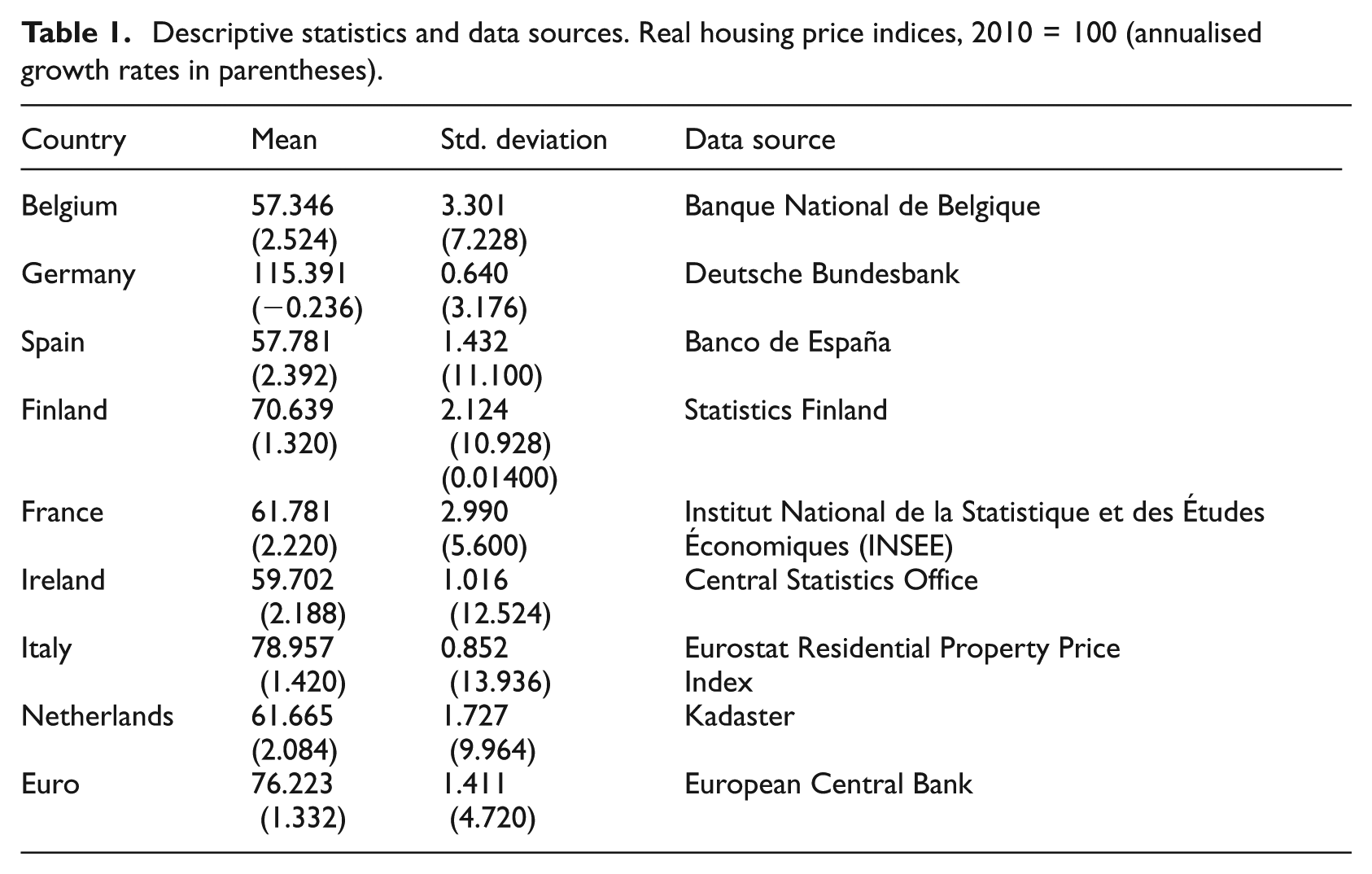
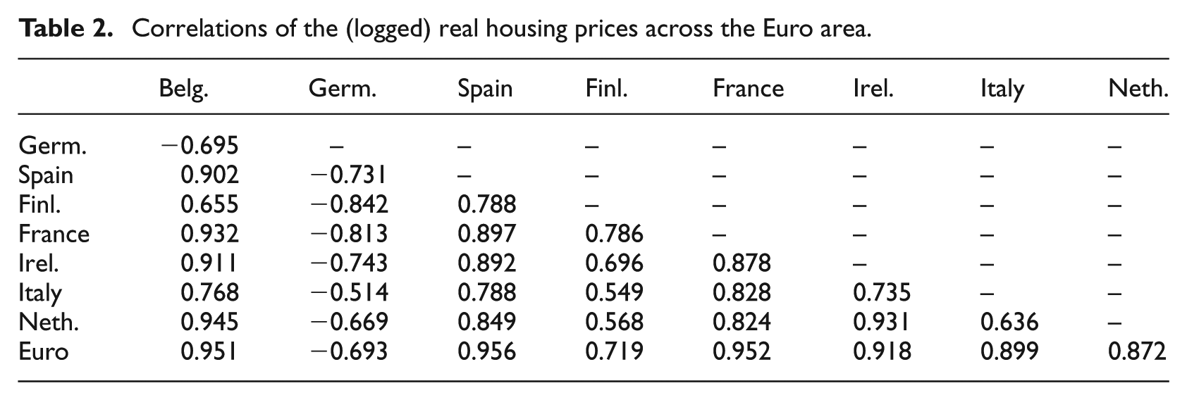
Between 1971 and 2012, real housing prices have increased on average at an annual rate of 1.3% in the Euro area, but with large differences across countries (Table 1). Most strikingly, prices declined on average by 0.2% in Germany, while they rose by at least 1.3% in all other countries, with increases exceeding 2% in the Netherlands, France, Ireland, Spain and Belgium. The standard deviation of growth rates has also varied markedly across countries, ranging from 3.2 to 13.9 percentage points, with a Euro-area average of 4.7. Volatility has been very low in Germany, moderate in Belgium and France and fairly high in the five other countries of the sample. Correlations between real housing price levels across the Euro area are generally strongly positive (Table 2). This is especially the case between Belgium, France, Ireland, the Netherlands and Spain. Prices in these countries are also positively correlated with those from Finland and Italy, although the link is somewhat weaker. Strikingly, German housing prices exhibit strong negative correlations with all other Euro area countries.

Table 2.

Correlations of the (logged) real housing prices across the Euro area.

	Belg.	Germ.	Spain	Finl.	France	Irel.	Italy	Neth.
Germ.	−0.695	–	–	–	–	–	–	–
Spain	0.902	−0.731	–	–	–	–	–	–
Finl.	0.655	−0.842	0.788	–	–	–	–	–
France	0.932	−0.813	0.897	0.786	–	–	–	–
Irel.	0.911	−0.743	0.892	0.696	0.878	–	–	–
Italy	0.768	−0.514	0.788	0.549	0.828	0.735	–	–
Neth.	0.945	−0.669	0.849	0.568	0.824	0.931	0.636	–
Euro	0.951	−0.693	0.956	0.719	0.952	0.918	0.899	0.872

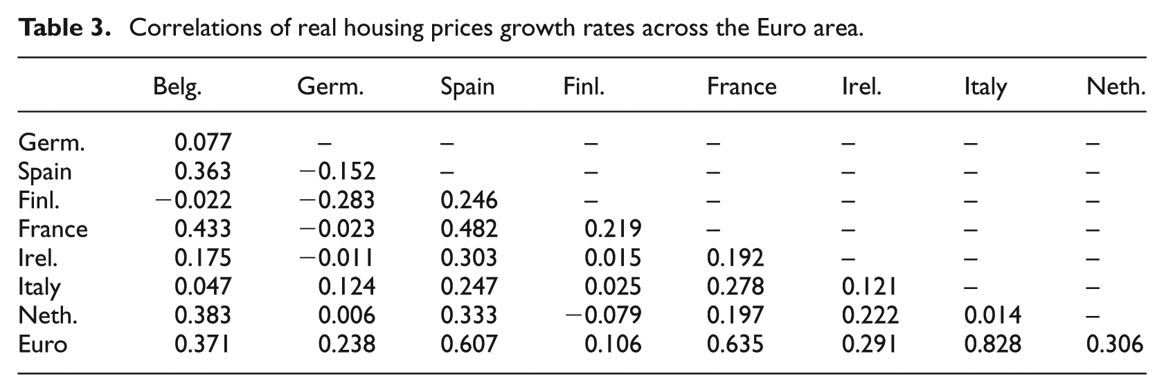
Although correlations between real housing price quarterly growth rates are weaker than between housing price levels, they are still high in some cases (Table 3). The strongest correlations with aggregate Euro area prices increases are in France, Spain and Italy. Bilateral correlations between price increases in these countries are also fairly high. Price increases in Belgium, France and the Netherlands also exhibit relatively strong correlation. For Ireland, the strongest correlation is with Spain, reflecting a recent boom-bust cycle in both countries, but correlations with France, Belgium and the Netherlands are also meaningful. For Finland, the correlation with the Euro area is low, although there is a significant negative correlation with Germany and a positive one with France and Spain. Finally, as for levels, Germany is special, with very low correlations with all other countries, except for a negative correlation with Finland and a positive one with the Euro area, which essentially reflects the weight of Germany itself in the aggregate.

Table 3.

Correlations of real housing prices growth rates across the Euro area.

	Belg.	Germ.	Spain	Finl.	France	Irel.	Italy	Neth.
Germ.	0.077	–	–	–	–	–	–	–
Spain	0.363	−0.152	–	–	–	–	–	–
Finl.	−0.022	−0.283	0.246	–	–	–	–	–
France	0.433	−0.023	0.482	0.219	–	–	–	–
Irel.	0.175	−0.011	0.303	0.015	0.192	–	–	–
Italy	0.047	0.124	0.247	0.025	0.278	0.121	–	–
Neth.	0.383	0.006	0.333	−0.079	0.197	0.222	0.014	–
Euro	0.371	0.238	0.607	0.106	0.635	0.291	0.828	0.306

Figures 1 and 2 depict the evolution of real housing prices in individual countries and the Euro area, respectively. While there are some common patterns, notably the large housing price increases in all countries except Germany in the run up to the global financial and economic crisis which started in 2007, a number of country-specific features emerge. First, bubbles have burst in several countries, in particular the Netherlands in the 1970s, Finland in the early 1990s and Ireland and Spain more recently. Second, the large increases that took place in most countries in the first part of the 2000s were followed by divergent evolutions. In Belgium, Finland and France, prices stabilised at a high level, as low interest rates supported demand and supply remained tight. In Ireland and Spain, prices fell sharply, reflecting oversupply of housing after huge construction booms in the years preceding the crisis. In Italy and the Netherlands, price falls have so far been more modest, reflecting the deterioration of economic conditions rather than bursting housing bubbles. Third, the negative correlation between housing prices in Germany and elsewhere in the Euro area still holds after the global financial crisis. While prices fell or at least decelerated in other countries, they started rising again in Germany.

Figure 1.

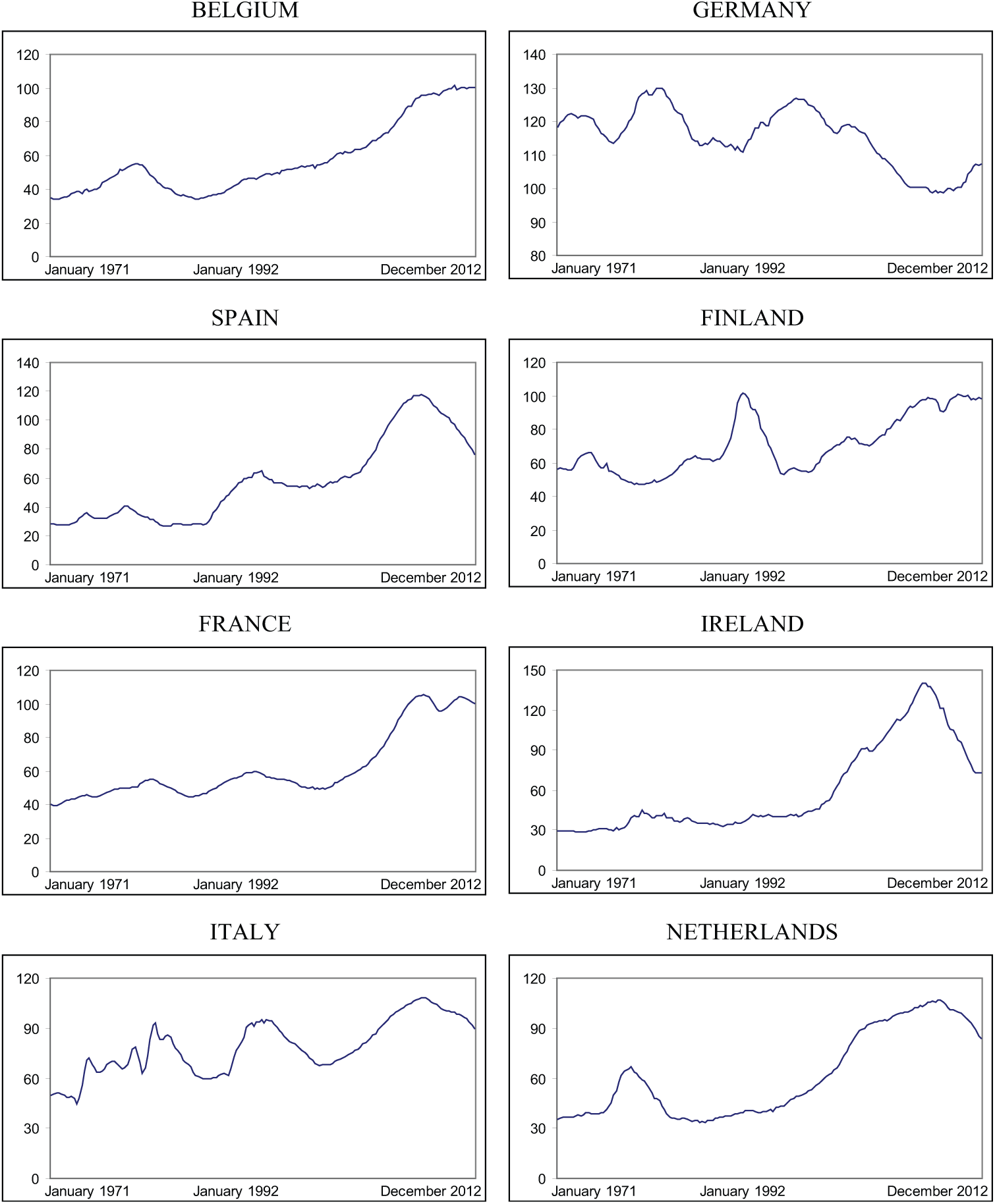
Real housing prices in the eight European countries and the aggregate Euro area. Original time series (indices, 2010 = 100).

Figure 2.

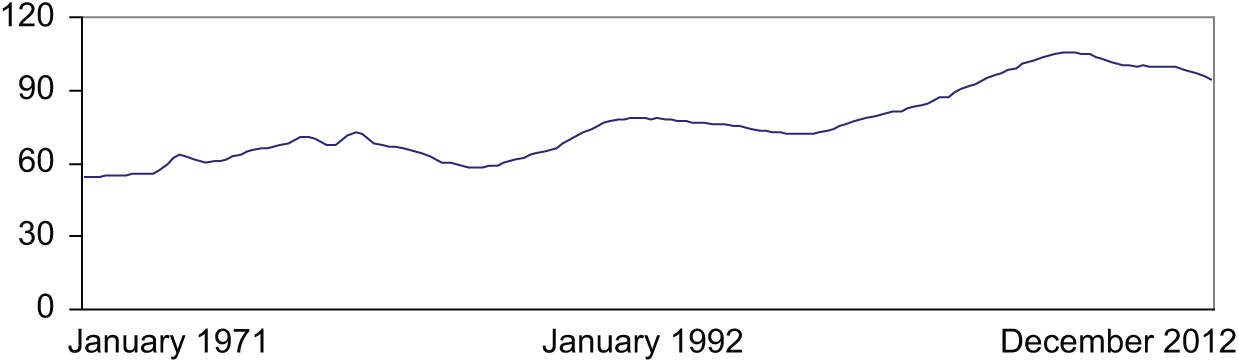
Real housing prices in the eight European countries and the aggregate Euro area. Original time series: Euro (index, 2010 = 100).

Methodology

The methodology employed in this paper to test comovement is based on the concepts of fractional integration and cointegration. We first need to introduce some definitions. A covariance stationary process {x_t, t = 0, ± 1, …} is integrated of order 0 (and denoted by I(0)) if the infinite sum of the autocovariances γ_u = E [(x_t − Ex_t)(x_t_+u − Ex_t)] is finite, i.e.:

\lim_{n \to \infty} \sum_{j = - n}^{n} | γ_{j} | < \infty .

(1)

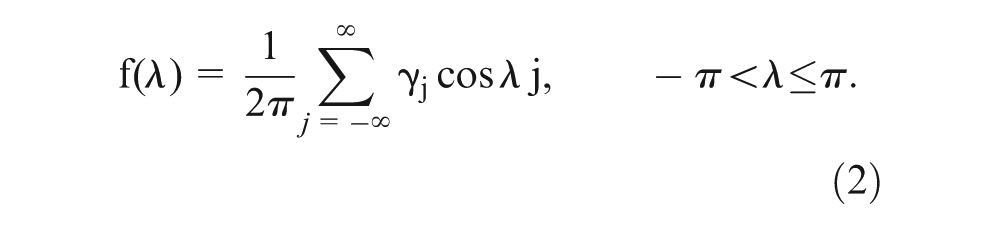
Alternatively, it can be defined in the frequency domain. Supposing that x_t has an absolutely continuous spectral distribution function, implying that it has a spectral density function, denoted by f(λ), and defined as:

f (λ) = \frac{1}{2 π} \sum_{j = - \infty}^{\infty} γ_{j} \cos λ j, - π < λ \leq π .

(2)

Then, x_t is I(0) if the spectral density function is positive and finite, i.e.:

0 < f (λ) < \infty, λ \in [0, π] .

(3)

A process is fractionally integrated, or integrated of order d (x_t≈I(d)) if:

{(1 - L)}^{d} x_{t} = u_{t}, t = 0, \pm 1, . . .,

(4)

where d can be any real value (and thus including fractional values), L is the lag-operator (Lx_t = x_t_-1) and u_t is I(0) as defined above.

Given the parameterisation in (4), the fractional differencing parameter d plays a crucial role. If d = 0, x_t = u_t, x_t is said to be ‘short memory’ or I(0), and if the observations are autocorrelated they are of a ‘weak’ form, in the sense that the values in the autocorrelations are decaying exponentially; if d > 0, x_t is said to be ‘long memory’, so named because of the strong association between observations far distant in time. Here, if d belongs to the interval (0, 0.5) x_t is still covariance stationary, while d ≥ 0.5 implies nonstationarity. Finally, if d < 1, the series is mean reverting in the sense that the effect of the shocks disappears in the long run, contrary to what happens if d ≥ 1, with shocks persisting forever.

Several methods exist for estimating and testing the fractional differencing parameter d. Some are parametric while others are semi-parametric and can be specified in the time or in the frequency domain. In this paper, we use a parametric Whittle estimation approach (Dahlhaus, 1989) along with a testing procedure (Robinson, 1994), which is based on the Lagrange Multiplier (LM) principle and uses the Whittle function in the frequency domain, as well as several semi-parametric methods (Abadir et al., 2007; Kim and Phillips, 1999, 2006; Robinson, 1995a, 1995b; Velasco, 1999a, 1999b).

The natural extension of fractional integration to the multivariate case is the concept of fractional cointegration. Engle and Granger (1987) suggested that, if two processes x_t and y_t are both I(d), then for a certain scalar α≠ 0, a linear combination w_t = y_t − αx_t, might be I(d − b) with b > 0.¹ This is the concept of cointegration, which they adapted from Granger (1981) and Granger and Weiss (1983). Given two real numbers d, b, the components of the vector z_t are said to be cointegrated of order d, b, denoted z_t∼CI(d, b) if:

all the components of z_t are I(d),

there exists a vector α≠ 0 such that s_t = α’z_t∼I(γ) = I(d − b), b > 0.

Here, α and s_t are called the cointegrating vector and error, respectively. Note that by allowing fractional degrees of differentiation, we allow a greater flexibility in representing equilibrium relationships between economic variables than the traditional use of integer differentiation.

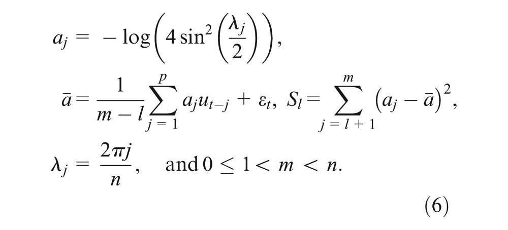
Here we conduct the following strategy: we first estimate individually the orders of integration of the series using, in addition to the previous methods, the log-periodogram-type of estimator as devised by Robinson (1995b), Kim and Phillips (1999, 2006), Velasco (1999b) and others. This method is a generalisation of the one proposed earlier by Geweke and Porter-Hudak (GPH, 1983), and is defined as:

\hat{d} (l) = \sum_{j = l + 1}^{m} (a_{j} - \bar{a}) \log I (λ_{j}) / S_{l},

(5)

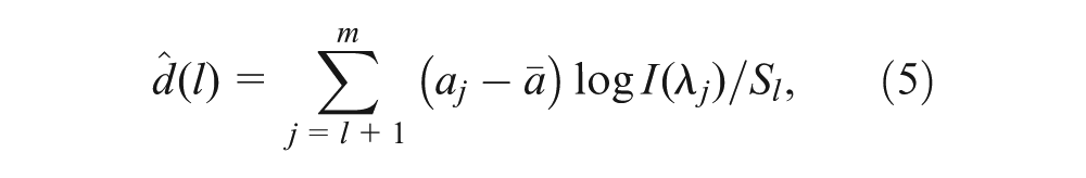
where

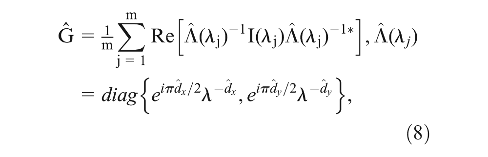
\begin{array}{l} a_{j} = - \log (4 \sin^{2} (\frac{λ_{j}}{2})), \\ \bar{a} = \frac{1}{m - l} \sum_{j = 1}^{p} a_{j} u_{t - j} + ε_{t}, S_{l} = \sum_{j = l + 1}^{m} {(a_{j} - \bar{a})}^{2}, \\ λ_{j} = \frac{2 π j}{n}, and 0 \leq 1 < m < n . \end{array}

(6)

Next we test the homogeneity of the orders of integration in the bivariate systems (i.e. H_o: d_x = d_y), where d_x and d_y are now the orders of integration of the two individual series, by using an adaptation of Robinson and Yajima (2002) statistic ${\hat{T}}_{xy}$ to log-periodogram estimation. The statistic is:

{\hat{T}}_{xy} = \frac{m^{1 / 2} ({\hat{d}}_{x} - {\hat{d}}_{y})}{{(\frac{1}{2} (1 - {\hat{G}}_{xy} / ({\hat{G}}_{xx} {\hat{G}}_{yy}))}^{1 / 2} + h (n)}

(7)

where h(n) > 0 and ${\hat{G}}_{xy}$ is the (xy)th element of:

\begin{array}{l} \hat{G} = \frac{1}{m} \sum_{j = 1}^{m} Re [\hat{Λ} {(λ_{j})}^{- 1} I (λ_{j}) \hat{Λ} {(λ_{j})}^{- 1 *}], \hat{Λ} (λ_{j}) \\ = d i a g {e^{i π {\hat{d}}_{x} / 2} λ^{- {\hat{d}}_{x}}, e^{i π {\hat{d}}_{y} / 2} λ^{- {\hat{d}}_{y}}}, \end{array}

(8)

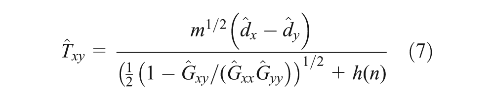
with a standard normal limit distribution (see Gil-Alana and Hualde, 2009, for evidence on the finite sample performance of this procedure). In the final step, we perform the Hausman test for no cointegration of Marinucci and Robinson (2001) comparing the estimate ${\hat{d}}_{x}$ of d_x with the more efficient bivariate one of Robinson (1995b), which uses the information that d_x = d_y = d_*. Marinucci and Robinson (2001) show that:

H_{im} = 8 m {({\hat{d}}_{*} - {\hat{d}}_{i})}^{2} \to_{d} χ_{1}^{2} as \frac{1}{m} + \frac{m}{n} \to 0,

(9)

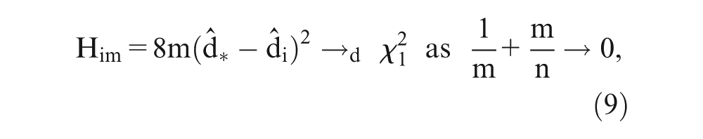
with i = x, y, and where m < [n/2] is again a bandwidth parameter, analogous to that introduced earlier; ${\hat{d}}_{i}$ are univariate estimates of the parent series, and ${\hat{d}}_{*}$ is a restricted estimate obtained in the bivariate context under the assumption that d_x = d_y. In particular:

{\hat{d}}_{*} = - \frac{\sum_{j = 1}^{s} 1_{2}' {\hat{Ω}}^{- 1} Y_{j} v_{j}}{21_{2}' {\hat{Ω}}^{- 1} 1_{2} \sum_{j = 1}^{s} v_{j}^{2}},

(10)

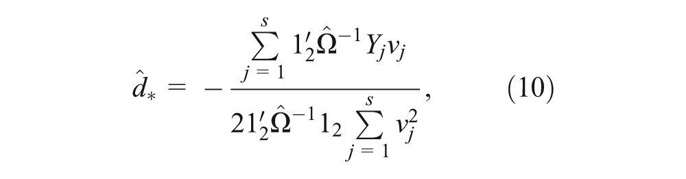
where 1₂ indicates a (2 × 1) vector of 1s, and with Y_j = [log I_xx(λ_j), log I_yy(λ_j)]^T, and $v_{j} = \log j - \frac{1}{s} \sum_{j = 1}^{s} \log j .$ The limiting distribution above is presented heuristically, but the authors argue that it seems sufficiently convincing for the test to warrant serious consideration.

Results

We start computing the univariate results and consider first the following model:

y_{t} = β_{0} + β_{1} t + x_{t}, {(1 - L)}^{d} x_{t} = u_{t}, t = 1, 2,

(11)

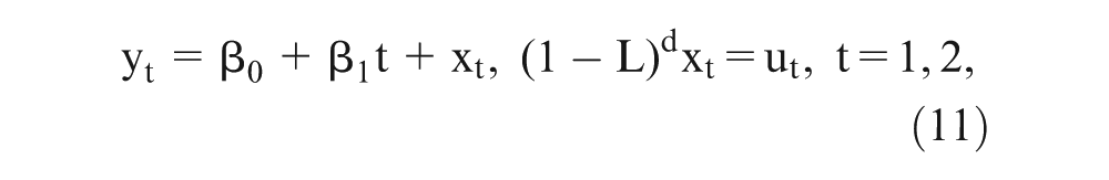
where y_t is the observed time series (log of the housing prices for each country), β₀ and β₁ are the coefficients corresponding to the intercept and a linear time trend, respectively, and the disturbance term u_t is assumed to be first a white noise process; then, we also admit the possibility of a weakly autocorrelated process. In the latter case, we use a non-parametric approximation from Bloomfield (1973) that approximates ARMA structures with a reduced number of parameters.²

Tables 4 and 5 display the estimated values of d, respectively for the two cases of white noise and Bloomfield autocorrelated disturbances. We consider the three standard cases examined in the literature, i.e. the case of no regressors (i.e. β₀ = β₁ = 0 a priori in equation (11)), an intercept (β₀ unknown, and β₁ = 0 a priori), and an intercept with a linear time trend (β₀ and β₁ unknown). Together with the Whittle estimates of the fractional differencing parameter, we also present the 95% confidence band of the non-rejection values of d, using Robinson’s (1994) parametric tests.

Table 4.

Estimates of d (and 95% intervals) with white noise disturbances.

Country	No regressors	An intercept	A linear time trend
Belgium	0.971	1.338	1.340
Belgium	(0.881, 1.092)	(1.264, 1.426)	(1.272, 1.427)
Germany	0.983	1.359	1.359
Germany	(0.895, 1.103)	(1.274, 1.470)	(1.274, 1.471)
Spain	0.965	1.594	1.594
Spain	(0.869, 1.092)	(1.503, 1.709)	(1.503, 1.710)
Finland	0.983	1.567	1.569
Finland	(0.893, 1.105)	(1.463 1.696)	(1.465, 1.700)
France	0.969	1.728	1.727
France	(0.881, 1.090)	(1.638, 1.836)	(1.637, 1.835)
Ireland	0.972	1.296	1.295
Ireland	(0.877, 1.099)	(1.226 1.386)	(1.226, 1.385)
Italy	0.971	1.797	1.797
Italy	(0.884, 1.092)	(1.515, 2.172)	(1.515, 2.176)
Netherlands	0.974	1.509	1.508
Netherlands	(0.883, 1.0955)	(1.435 1.600)	(1.435, 1.601)
Euro	0.971	1.783	1.784
Euro	(0.881, 1.093)	(1.617, 2.013)	(1.618, 2.020)

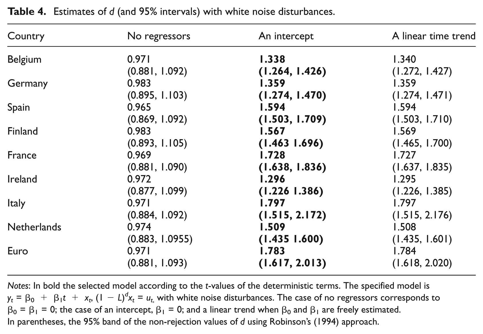
Notes: In bold the selected model according to the t-values of the deterministic terms. The specified model is y_t = β₀ + β₁t + x_t, (1 − L)^dx_t = u_t, with white noise disturbances. The case of no regressors corresponds to β₀ = β₁ = 0; the case of an intercept, β₁ = 0; and a linear trend when β₀ and β₁ are freely estimated.

In parentheses, the 95% band of the non-rejection values of d using Robinson’s (1994) approach.

Table 5.

Estimates of d (and 95% intervals) with autocorrelated (Bloomfield) errors.

Country	No regressors	An intercept	A linear time trend
Belgium	0.921	1.618	1.609
Belgium	(0.787, 1.143)	(1.422, 1.856)	(1.431, 1.847)
Germany	0.943	1.399	1.399
Germany	(0.801, 1.178)	(1.213, 1.601)	(1.212, 1.667)
Spain	0.908	1.699	1.699
Spain	(0.732, 1.105)	(1.601, 2.006)	(1.502, 2.031)
Finland	0.943	1.567	1.578
Finland	(0.809, 1.143)	(1.319 1.908)	(1.313, 1.947)
France	0.928	1.994	1.971
France	(0.789, 1.144)	(1.722, 2.353)	(1.723, 2.374)
Ireland	0.906	1.469	1.469
Ireland	(0.749, 1.151)	(1.324 1.684)	(1.318, 1.676)
Italy	0.921	0.875	0.882
Italy	(0.784, 1.144)	(0.696, 1.112)	(0.711, 1.116)
Netherlands	0.933	1.862	1.859
Netherlands	(0.789, 1.132)	(1.643 2.190)	(1.644, 2.164)
Euro	0.936	1.319	1.319
Euro	(0.792, 1.148)	(1.141, 1.570)	(1.146, 1.571)

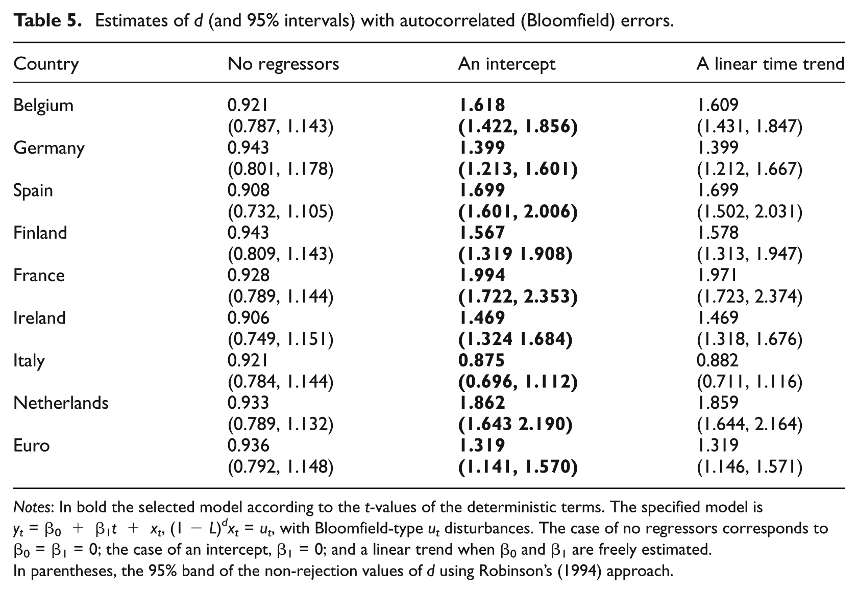
Notes: In bold the selected model according to the t-values of the deterministic terms. The specified model is y_t = β₀ + β₁t + x_t, (1 − L)^dx_t = u_t, with Bloomfield-type u_t disturbances. The case of no regressors corresponds to β₀ = β₁ = 0; the case of an intercept, β₁ = 0; and a linear trend when β₀ and β₁ are freely estimated.

In parentheses, the 95% band of the non-rejection values of d using Robinson’s (1994) approach.

The first thing we observe across these tables is that (according to the t-values of the deterministic terms, unreported) the most plausible models are those including only an intercept, and the estimated values of d are statistically significantly above 1 in practically all cases.³ In fact, the only exception is Italy with autocorrelated errors, where the unit root null hypothesis (d = 1) cannot be rejected. In all the other cases, including the Euro area, this hypothesis is decisively rejected in favour of d > 1. An obvious implication of the above result is that the series are highly persistent. Moreover, the fact that the series have been analysed in logs implies that their corresponding growth rates (i.e. their first differences) are long memory (i.e. d > 0), with shocks affecting them taking a long time to disappear completely.⁴

Next we focus on the bivariate relationships between each of the individual series and the Euro. A necessary condition for cointegration is that the two parent series must share the same degree of integration. Then, looking at the confidence intervals reported in the tables, we can remove some of these relationships. For instance, in Table 4, the range of values of d for the Euro is between 1.617 and 2.013. Thus, any interval that does not overlap with this one (either from below or from above) will indicate that the two series cannot be cointegrated. This happens for Belgium, Germany, Ireland and the Netherlands where the intervals are strictly on the left of the Euro interval. However, for the remaining series (Spain, Finland, France and Italy) the intervals overlap so the homogeneity condition for the orders of integration may be satisfied. Focusing on the case of autocorrelated errors (in Table 5) we get the opposite result and we see that, according to the confidence bands, the homogeneity condition of equal orders of integration may be satisfied in the cases of Belgium, Germany, Finland and Ireland, and should be ruled out for Spain, France, Italy and the Netherlands. Thus, apparently, this result is just the opposite to the one obtained with the white noise disturbances in Table 4. The only country where results are consistent across specifications with white noise and autocorrelated errors is the Netherlands, where the order of integration is significantly different from that of the Euro area.

The disparity in the results presented when using the parametric methods (depending on whether the errors are uncorrelated or autocorrelated) might be a consequence of the relatively small sample size used in the application (n = 168). In order to solve this problem we use a semi-parametric approach where no structure is imposed on the error term. Here we use an approach proposed in Robinson (1995a), which is a ‘local’ Whittle estimate in the frequency domain, based on a band of frequencies that degenerates to zero. It is implicitly defined by: $\hat{d} = \arg \min_{d} (\log \bar{C (d)} - 2 d \frac{1}{m} \sum_{j = 1}^{m} \log λ_{j}),$ for $d \in (- 1 / 2, 1 / 2); \bar{C (d)} = \frac{1}{m} \sum_{j = 1}^{m} I (λ_{j}) λ_{j}^{2 d},$

λ_{j} = \frac{2 π j}{T}, \frac{1}{m} + \frac{m}{n} \to 0,

(12)

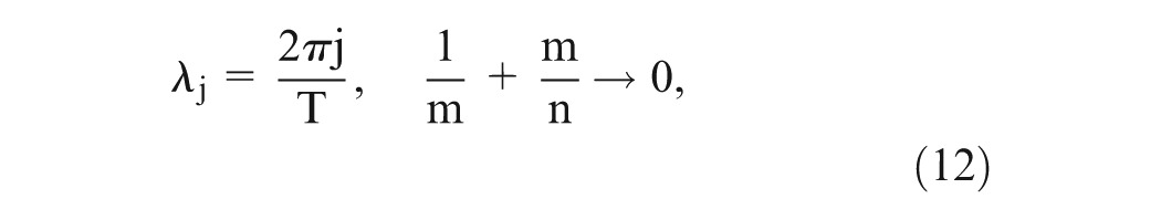
where m is the bandwidth parameter, and I(λ_j) is the periodogram of the time series, x_t, given by:

I (λ_{j}) = \frac{1}{2 π n} {| \sum_{t = 1}^{n} x_{t} e^{i λ_{j} t} |}^{2} .

(13)

Under finiteness of the fourth moment and other mild conditions, Robinson (1995a) proved that:

\sqrt{m} (\hat{d} - d_{o}) \to_{d} N (0, 1 / 4) as n \to \infty,

(14)

where d_o is the true value of d and with the only additional requirement that m →∞ slower than n.

The results based on this approach are displayed in Table 6. Given the nonstationary nature of the series, the results are based on the first (or second) differenced series, adding 1 (or 2) to the estimated obtained values. This is a standard practice in most of the semi-parametric methods. Nevertheless, Velasco and Robinson (2000), Phillips and Shimotsu (2004, 2005), Abadir et al. (2007) and others proposed an extension of this method by means of tapering that is valid in nonstationary contexts. Using some of these methods (Abadir et al., 2007; Velasco and Robinson, 2000) the results were practically identical to those reported here. They indicate again that most of the estimates are substantially higher than 1. If we focus on the bandwidth number m = (n)^0.5 (which is the one used in most of the empirical works) the estimate for the Euro is 1.628, and Finland and Italy are the only two countries where we observe large deviations from this number. The orders of integration of Belgium, Germany, Spain, France, Ireland and the Netherlands seem to be of a similar magnitude as the one for the Euro, a condition required to test for cointegration. Nevertheless, in what follows we conduct a proper statistical test for testing the homogeneity condition on the orders of integration of the series.

Table 6.

Semi-parametric Whittle estimates of d for different bandwidth numbers.

Country	5	8	10	13	15	20	30
Belgium	0.916	1.452	1.651*	1.583*	1.695*	1.834*	1.686*
Germany	0.789	1.180	1.225	1.566*	1.641*	1.451	1.612*
Spain	0.818	1.442	1.359	1.424	1.540*	1.475	1.658*
Finland	0.500	0.604	0.871	1.274	1.262	1.428	1.598*
France	0.977	1.321	1.333	1.495	1.521	1.661*	1.850*
Ireland	1.268	1.667*	1.684*	1.446	1.483	1.457	1.454
Italy	0.500	0.790	1.349	1.237	1.208	0.929	0.980
Netherlands	1.023	1.187	1.422	1.580*	1.483	1.781*	1.913*
Euro	0.500	1.654*	1.539*	1.628*	1.614*	1.263	1.379

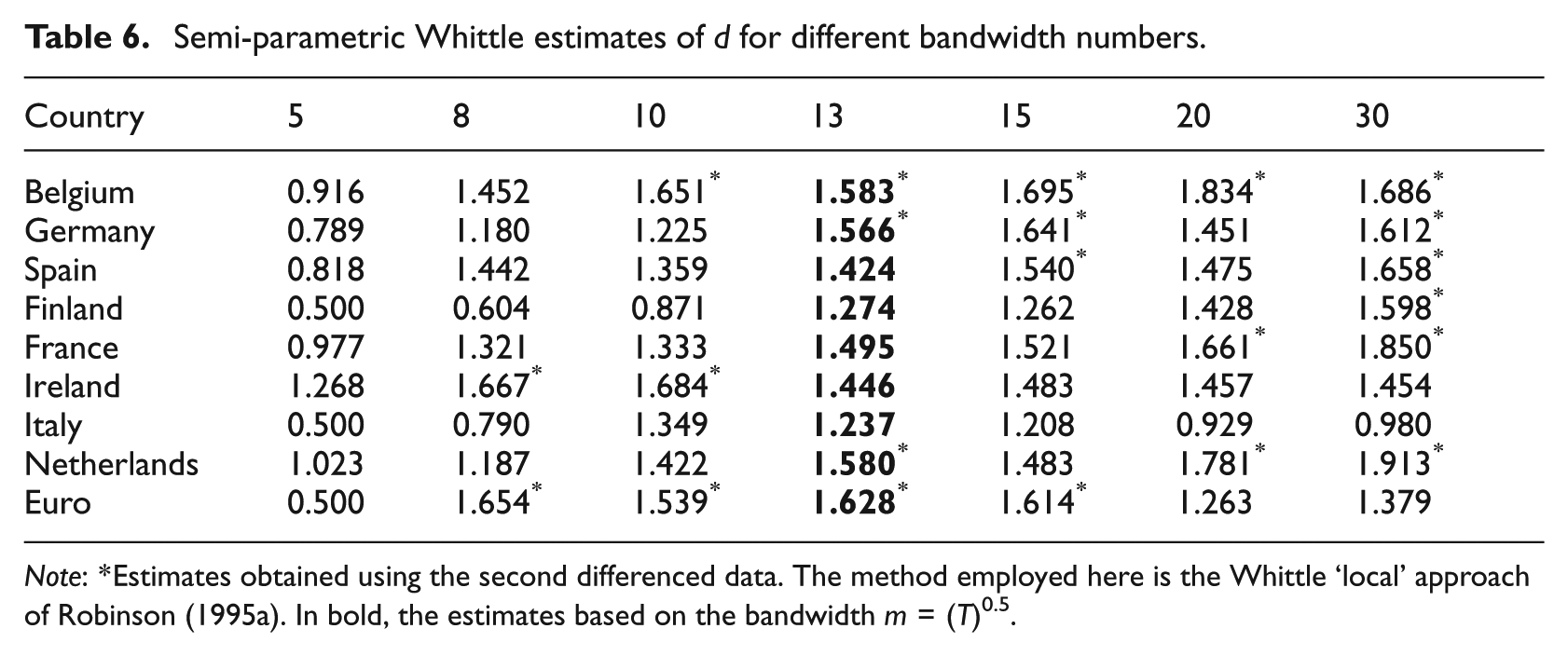
Note: *Estimates obtained using the second differenced data. The method employed here is the Whittle ‘local’ approach of Robinson (1995a). In bold, the estimates based on the bandwidth m = (T)^0.5.

Table 7 reports the statistics obtained when testing the homogeneity condition in a pairwise representation through the Robinson and Yajima (2002) approach as presented in the previous section. If we look first at the bottom row in the table (referring to the Euro), we observe that only for Finland and Italy do we obtain statistically different orders of integration with respect to that of the Euro. This is consistent with the semi-parametric results displayed in Table 6. The homogeneity condition is satisfied in the following cases: Belgium presents a similar order of integration as Germany, Spain, France, Ireland and the Netherlands; the order of integration of Germany is consistent with Belgium, Spain, France, Ireland and the Netherlands; the orders of integration of Spain and Ireland are consistent with all the other countries; Finland presents similar orders of integration as France, Ireland, Italy and Spain, but different from those of Belgium, Germany and the Netherlands. Italy displays similar degrees of integration as Spain, Finland and Ireland, but different from those of Belgium, Germany, the Netherlands and France; the order of integration of France is consistent with all except Italy, and the one in the Netherlands with all except Finland and Italy.

Table 7.

Testing for the homogeneity condition in the order of integration.

	Belg.	Germ.	Spain	Finl.	France	Irel.	Italy	Neth.
Germ.	0.118	–	–	–	–	–	–	–
Spain	1.105	0.986	–	–	–	–	–	–
Finl.	2.147*	2.029*	1.042	–	–	–	–	–
France	0.611	0.493	0.491	1.536	–	–	–	–
Irel.	0.952	0.834	0.152	1.195	0.340	–	–	–
Italy	2.404*	2.286*	1.299	0.257	1.793*	1.452	–	–
Neth.	0.020	0.097	1.083	2.126*	0.590	0.931	2.383*	–
Euro	0.312	0.431	1.417	3.460*	0.924	1.264	2.717*	0.312

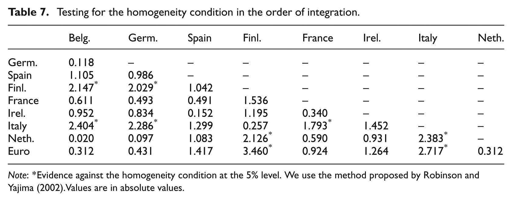
Note: *Evidence against the homogeneity condition at the 5% level. We use the method proposed by Robinson and Yajima (2002).Values are in absolute values.

Table 8 displays the results of testing the null hypothesis of no cointegration against the alternative of fractional cointegration through the Hausman test of Marinucci and Robinson (2001). The first two values in each case correspond to the test statistics relative to each individual series (i.e. equation (9) with i = x and i = y, respectively), while the lowest value is the estimate of d obtained in the bivariate representation of the series under the assumption of equal orders of integration.

Table 8.

Testing the null of no cointegration against fractional cointegration.

x/y	Belg.	Germ.	Spain	Finl.	France	Irel.	Italy	Neth.
Germ.	1.698	–	–	–	–	–	–	–
	2.159
	1.433
Spain	4.113*	5.617*	–	–	–	–	–	–
	12.859*	13.428*
	1.217	1.192
Finl.	N.A.	N.A.	0.760	–	–	–	–	–
			0.357
			1.363
France	1.881	2.582	11.559*	0.075	–	–	–	–
	4.990*	6.096*	7.312*	3.575
	1.355	1.331	1.148	1.467
Irel.	2.159	4.562*	2.457	0.034	2.873	–	–	–
	7.907*	10.967*	1.828	2.645	4.731*
	1.296	1.228	1.286	1.440	1.273
Italy	N.A.	N.A.	0.629	0.540	N.A.	0.311	–	–
			6.895*	0.138		2.217
			1.156	1.312		1.294
Neth.	10.773*	0.470	2.613	N.A.	1.723	25.264*	N.A.	–
	10.967*	0.301	0.077		0.230	13.789*
	1.245	1.510	1.415		1.446	1.067
Euro	29.040*	7.050*	7.580*	N.A.	25.165*	5.301*	N.A.	3.205
	24.482*	4.193*	0.569		13.789*	0.269		1.801
	1.078	1.357	1.347		1.116	1.393		1.443

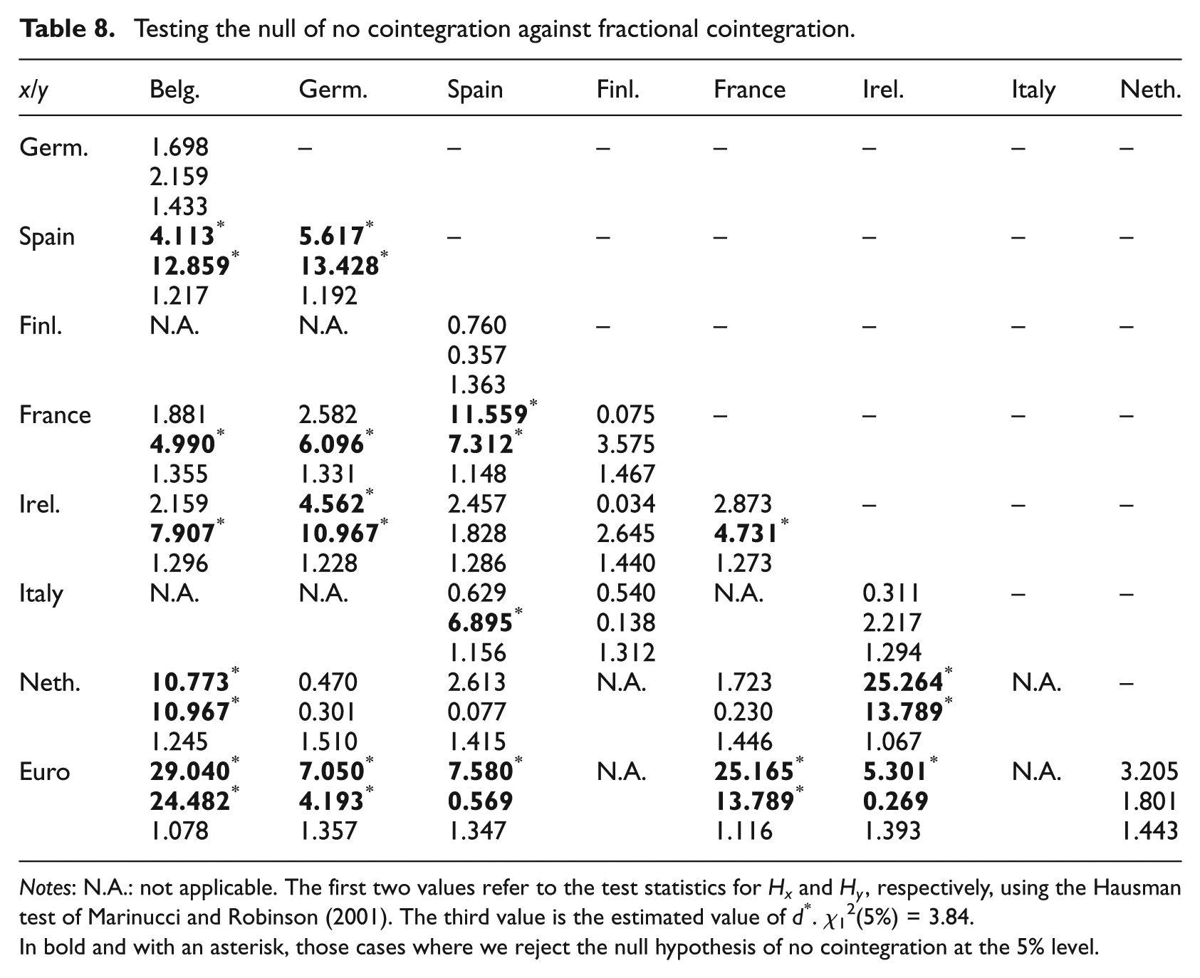
Notes: N.A.: not applicable. The first two values refer to the test statistics for H_x and H_y, respectively, using the Hausman test of Marinucci and Robinson (2001). The third value is the estimated value of d^*. χ₁²(5%) = 3.84.

In bold and with an asterisk, those cases where we reject the null hypothesis of no cointegration at the 5% level.

Starting with the comparisons with respect to the Euro, we observe evidence of cointegration in the cases of Belgium, Germany and France, and ambiguous results are obtained in the cases of Spain and Ireland where only statistical differences are obtained in one of the two series. Focusing on the individual countries, Spain seems to be cointegrated with Belgium, Germany and France, and clearly does not cointegrate with Ireland and the Netherlands; Germany cointegrates with Spain and Ireland, and Belgium cointegrates with Spain and the Netherlands but does not cointegrate with Germany. Finally, the Netherlands also cointegrates with Ireland. For the remaining cases, there is no cointegration or the results are ambiguous in the sense that the hypothesis of no cointegration can be rejected with respect to only one of the two series.

A final issue that deserves attention is the fact that since the individual housing prices series are nonstationary, with orders of integration greater than 1 in practically all cases, and the cointegrating relationships are in all cases lower but still above 1, this implies that the series diverge in the long run. On the other hand, the fact that the analysis has been conducted on the logged-transformed series indicates that it is the growth rate of the series that in fact cointegrate in the long run, showing thus the existence of comovements in the data.

The finding of some comovement in housing price growth rates across the Euro area, but with significant differences between countries is consistent with the findings from Vansteenkiste and Hiebert (2011) (hereafter VH) showing limited and heterogeneous housing price spillovers in the Euro area. Although the results are not directly comparable, as VH study the impact of housing shocks in a GVAR model, other common patterns emerge. VH find a relation between housing price spillovers and geographic proximity. In particular, the link between housing prices in Belgium and the Netherlands found in VH is consistent with our finding of a strong cointegration relationship between these countries. The same holds for France and Spain, whose synchronisation in housing cycles is also documented in Ferrara and Koopman (2010).

Concluding remarks

In this paper we have examined comovement between housing prices across the Euro area by means of fractional integration and cointegration techniques. The results indicate first that the orders of integration of the individual series, corresponding to the logarithms of quarterly real housing prices from 1971 until 2012, are strictly above 1 in all cases, implying that the growth rate series (i.e. their first differences) display long memory behaviour. Focusing on the bivariate relationships we observe that the orders of integration corresponding to the data for Finland and Italy present the highest disparities with respect to the Euro area and the remaining countries, and evidence of fractional cointegration with respect to the Euro area seems to be obtained in the cases of Belgium, Germany and France.

Several other issues also deserve attention. First, cointegration takes place in the growth rates series and is relatively weak, implying very slow convergence. Note that all logged individual series display orders of integration which are significantly above 1 and even the cointegrating relationships present estimates above 1. Thus, the cointegrating relationship takes place on the first differenced series, which are the growth rates. For example, looking at the results displayed in Tables 6 (with m = 13) and 8 (bottom values in the last row) and focusing on the Euro (and the countries that cointegrate with it, Belgium, Germany and France) the orders of integration of the growth rates series are, respectively, 0.628 (Euro), 0.583, 0.566 and 0.495, and those of their corresponding cointegrating relations are 0.078 (Belgium), 0.357 (Germany) and 0.116 (France).

A second important issue is the case of Germany. As noted earlier, the correlation coefficients between real housing prices among Euro area countries are strongly positive, except for those involving Germany. This is consistent with the fact that housing prices were falling in Germany during the global housing boom that took place between the mid 1990s and the economic and financial crisis which started in 2007. Since mid 2008, prices have risen significantly in Germany, while they have fallen or stagnated in the rest of the Euro area. This may be related to capital flowing back from the periphery of the Euro area to Germany, which is seen as a safe haven. Part of this capital could find its way to the housing market. After nearly two decades of real price decline, the German housing market looks attractive for investors and safe for mortgage lenders, which could explain rising demand, driving prices up. This interpretation seems consistent with the observation that housing prices in Ireland and Spain, two of the countries where large capital inflows have fuelled housing bubbles over the past decade, clearly exhibit cointegration with German prices. Further research would, however, be necessary to validate this interpretation of our results. In particular, the causality links between capital flows and housing prices, and the potential influences of third factors will require further investigation.

Footnotes

Acknowledgements

Comments from the Editor and three anonymous referees are gratefully acknowledged.

Funding

This research received no specific grant from any funding agency in the public, commercial, or not-for-profit sectors.

Notes

References

Abadir

Distaso

Giraitis

(2007) Nonstationarity-extended local Whittle estimation. Journal of Econometrics141: 1353–1384.

Alexander

Barrow

(1994) Seasonality and cointegration of regional house prices in the UK. Urban Studies31: 1667–1689.

Alvarez

Bulligan

Cabrero

. (2010) Housing cycles in the major Euro area countries. In: de Bandt

Knetsch

Peñalosa

(eds) Housing Markets in Europe. Springer, pp. 85–103.

André

(2010) A Bird"s Eye View of OECD Housing Markets. OECD Economics Department Working Papers, No. 746, OECD Publishing.

André

Gupta

Kanda

(2012) Do house prices impact consumption and interest rate? Evidence from OECD countries using an agnostic identification procedure. Applied Economics Quarterly58(1): 19–70.

Apergis

Payne

(2012) Convergence in U.S. housing prices by state: Evidence from the club convergence and clustering procedure. Letters in Spatial and Resource Sciences5(2): 103–111.

Balcilar

Beyene

Gupta

(2013) ‘Ripple’ effects in South African house prices. Urban Studies50(5): 876–894.

Barker

(2006) Barker Review of Land Use Planning. Final Report – Recommendations. London: HM Treasury.

Barros

Gil-Alana

Payne

(2012) Comovements among U.S. state housing prices: Evidence from fractional cointegration. Economic Modelling29: 936–942.

10.

Benjamin

Chinloy

Jud

(2004) Real estate versus financial wealth in consumption. Journal of Real Estate Finance and Economics29: 341–354.

11.

Bloomfield

(1973) An exponential model in the spectrum of a scalar time series. Biometrika60: 217–226.

12.

Building Societies Association (2007) House Price Expectations: an Insight into How People Think about Property Purchase. London: Building Societies Association.

13.

Burger

Van Rensburg

(2008) Metropolitan house prices in South Africa: Do they converge?South African Journal of Economics76: 291–297.

14.

Caldera

Johansson

(2013) The price responsiveness of housing supply in OECD countries. Journal of Housing Economics22(3): 231–249.

15.

Cameron

Muellbauer

Murphy

(2006) Was There a British House Price Bubble? Evidence from a Regional Panel. Centre for Economic Policy Research Discussion Paper, No. 5619.

16.

Campbell

Cocco

(2007) How do house prices affect consumption? Evidence from micro data. Journal of Monetary Economics54: 591–621.

17.

Canarella

Miller

Pollard

(2012) Unit roots and structural change: An application to US house-price indices. Urban Studies49(4): 757–776.

18.

Case

Quigley

Shiller

(2005) Comparing wealth effects: The stock market versus the housing market. Advances in Macroeconomics5: 1–32.

19.

Catte

Girouard

Price

(2004) Housing Markets, Wealth and the Business Cycle. OECD Economics Department Working Paper, No. 394, OECD Publishing.

20.

Cecchetti

(2008) Measuring the macroeconomic risks posed by asset price booms. In Campbell

(ed.) Asset Prices and Monetary Policy. Chicago, IL: University of Chicago Press, pp. 9–43.

21.

Claessens

Kose

Terrones

(2008) What Happens During Recessions, Crunches and Busts?International Monetary Fund Working Paper08/274, Washington, DC.

22.

Cook

(2003) The convergence of regional house prices in the UK. Urban Studies40: 2285–2294.

23.

Cook

(2005) Regional house price behavior in the UK: Application of a joint testing procedure. Physica A345: 611–621.

24.

Dahlhaus

(1989) Efficient parameter estimation for self-similar process. Annals of Statistics17: 1749–1766.

25.

de Bandt

Barhoumi

Bruneau

(2010) The international transmission of house price shocks. In: de Bandt

Knetsch

Peñalosa

(eds) Housing Markets in Europe. Springer, pp. 129–158.

26.

Detken

Smets

(2004) Asset Price Booms and Monetary Policy. European Central Bank Working Paper, No. 364.

27.

Engle

Granger

CWJ

(1987) Cointegration and error correction model. Representation, estimation and testing. Econometrica55: 251–276.

28.

European Central Bank (2005) Asset price bubbles and monetary policy. European Central Bank Monthly BulletinApril.

29.

Ferrara

Koopman

(2010) Common business and housing market cycles in the Euro area from a multivariate decomposition. In: de Bandt

Knetsch

Peñalosa

(eds) Housing Markets in Europe. Springer, pp. 105–128.

30.

Ferrero

(2012) House Price Booms, Current Account Deficits, and Low Interest Rates. Federal Reserve Bank of New York Staff Report, No. 541.

31.

Gete

(2009). Housing Markets and Current Account Dynamics. MPRA Paper 20957, University Library of Munich.

32.

Geweke

Porter-Hudak

(1983) The estimation and application of long memory time series models. Journal of Time Series Analysis4: 221–238.

33.

Gil-Alana

(2004) The use of the Bloomfield model as an approximation to ARMA processes in the context of fractional integration. Mathematical and Computer Modelling39: 429–436.

34.

Gil-Alana

Hualde

(2009) Fractional integration and cointegration. An overview with an empirical application. The Palgrave Handbook of Applied Econometrics2: 434–472.

35.

Girouard

Kennedy

Van den Noord

. (2006) Recent House Price Developments: The Role of Fundamentals. OECD Economics Department Working Papers, No. 475, OECD Publishing.

36.

Goodhart

Hofmann

(2008) House prices, money, credit, and the macroeconomy. Oxford Review of Economic Policy24(1): 180–205.

37.

Granger

CWJ

(1981) Some properties of time series data and their use in econometric model specification. Journal of Econometrics16: 121–130.

38.

Granger

CWJ

Weiss

(1983) Time series analysis of error-correcting models. In: Karlin

Amemiya

Goodman

(eds) Studies in Econometrics, Time Series and Multivariate Statistics. New York: Academic Press, pp. 255–278.

39.

Gupta

Miller

(2012a) ‘Ripple effects’ and forecasting home prices in Los Angeles, Las Vegas, and Phoenix. The Annals of Regional Science48(3): 763–782.

40.

Gupta

Miller

(2012b) The time series properties of house prices: A case study of the southern California market. Journal of Real Estate Finance and Economics44(3): 339–361.

41.

Holmes

Grimes

(2008) Is there long-run convergence among regional house prices in the UK?Urban Studies45: 1531–1544.

42.

Holmes

Otero

Panagiotidis

(2011) Investigating regional house price convergence in the United States: Evidence from a pair-wise approach. Economic Modelling28: 2369–2376.

43.

Iacoviello

Neri

(2010) Housing market spillovers: Evidence from an estimated DSGE model. American Economic Journal: Macroeconomics2: 125–164.

44.

Igan

Loungani

(2012) Global Housing Cycles. International Monetary Fund Working Paper12/217, Washington, DC.

45.

International Monetary Fund (2011) Housing Finance and Financial Stability – Back to Basics?Global Financial Stability Report, April, Washington, DC: International Monetary Fund.

46.

Jarocinski

Smets

(2008) House Prices and the Stance of Monetary Policy. European Central Bank Working Paper, No. 891.

47.

Kim

Phillips

PCB

(1999) Fully-Modified Estimation of Fractional Cointegration Models. Mimeo, Yale University.

48.

Kim

Phillips

PCB

(2006) Log Periodogram Regression: The Nonstationary Case. Cowles Foundation Discussion Papers, Cowles Foundation for Research in Economics, Yale University1587 pp.

49.

Larraz-Iribas

Alfaro-Navarro

(2008) Asymmetric behaviour of Spanish regional house prices. International Advances in Economic Research14: 407–421.

50.

Leamer

(2007) Housing is the business cycle. Economic Policy Symposium – Jackson Hole, Proceedings. Federal Reserve Bank of Kansas City, pp. 149–233.

51.

Lean

Smyth

(2013) Regional house prices and the ripple effect in Malaysia. Urban Studies50(5): 895–922.

52.

Lettau

Ludvigson

(2004) Understanding trend and cycle in asset values: Reevaluating the wealth effect on consumption. American Economic Review94(1): 276–299.

53.

Ludwig

Sløk

(2004) The relationship between stock prices, house prices and consumption in OECD countries. The B.E. Journal of Macroeconomics, De Gruyter4(1): 1–28.

54.

Luo

Liu

Picken

(2007) Housing price diffusion patterns of Australia"s state capital cities. International Journal of Strategic Property Management11: 227–242.

55.

MacDonald

Taylor

(1993) Regional house prices in Britain: Long-run relationships and short-run dynamics. Scottish Journal of Political Economy40: 43–55.

56.

Marinucci

Robinson

(2001) Semiparametric fractional cointegration analysis. Journal of Econometrics105: 225–247.

57.

Meen

(1999) Regional house prices and the ripple effect: A new interpretation. Housing Studies14: 733–753.

58.

Meen

(2008) Ten new propositions in UK housing macroeconomics: An overview of the first years of the century. Urban Studies45(13): 2759–2781.

59.

Miles

Pillonca

(2008) Financial innovation and European housing and mortgage markets. Oxford Review of Economic Policy24(1): 145–175.

60.

Muellbauer

Murphy

(2008) Housing markets and the economy: The assessment. Oxford Review of Economic Policy24(1): 1–33.

61.

Musso

Neri

Stracca

(2011) Housing, consumption and monetary policy: How different are the US and the Euro area?Journal of Banking and Finance35(11): 3019–3041.

62.

Obstfeld

Rogoff

(2009) Global Imbalances and the Financial Crisis: Products of Common Causes. CEPR Discussion Papers 7606. London: Centre for Economic Policy Research.

63.

Oikarinen

(2006) The diffusion of housing price movements from centre to surrounding areas. Journal of Housing Research15: 3–28.

64.

Payne

(2012) The long-run relationship between U.S. regional housing prices: An empirical note. Journal of Regional Analysis and Policy42(1): 28–35.

65.

Pollakowski

Ray

(1997) Housing price diffusion patterns at different aggregation levels: An examination of housing market efficiency. Journal of Housing Research8: 107–124.

66.

Phillips

PCB

Shimotsu

(2004) Local Whittle estimation in nonstationary and unit root cases. Annals of Statistics32: 656–692.

67.

Phillips

PCB

Shimotsu

(2005) Exact local Whittle estimation of fractional integration. Annals of Statistics33(4): 1890–1933.

68.

Reinhart

Rogoff

(2009) This Time is Different, Eight Centuries of Financial Folly. Princeton, NJ: Princeton University Press.

69.

Robinson

(1994) Efficient tests of nonstationary hypotheses. Journal of the American Statistical Association89: 1420–1437.

70.

Robinson

(1995a) Gaussian semi-parametric estimation of long range dependence. Annals of Statistics23: 1630–1661.

71.

Robinson

(1995b) Log-periodogram regression of time series with long range dependence. Annals of Statistics23: 1048–1072.

72.

Robinson

Yajima

(2002) Determination of cointegrating rank in fractional systems. Journal of Econometrics106: 217–241.

73.

Shiller

(2007) Understanding Recent Trends in House Prices and Home Ownership. NBER Working Papers, No. 13553.

74.

Vansteenkiste

(2007) Regional Housing Market Spillovers in the US: Lessons from Regional Divergences in a Common Monetary Policy Setting. European Central Bank Working Paper, No. 708.

75.

Vansteenkiste

Hiebert

(2011) Do house price developments spill over across Euro area countries? Evidence from a global VAR. Journal of Housing Economics20(4): 299–314.

76.

Velasco

(1999a) Gaussian semiparametric estimation of nonstationary time series. Journal of Time Series Analysis20: 87–127.

77.

Velasco

(1999b) Nonstationary log-periodogram regression. Journal of Econometrics91: 299–323.

78.

Velasco

Robinson

(2000) Whitle pseudo maximum likelihood estimation for nonstationary time series. Journal of the American Statistical Association95: 1229–1243.

79.

Zohrabyan

Leatham

Bessler

(2008) Cointegration analysis of regional house prices in the U.S. Proceedings, 2007 Agricultural and Rural Finance Markets in Transition. 4–5October2007, St. Louis, Missouri from Regional Research Committee NC-1014: Agricultural and Rural Finance Markets in Transition (unpublished).