Varying influences of the built environment on household travel in 15 diverse regions of the United States

Abstract

This study pools household travel and built environment data from 15 diverse US regions to produce travel models with more external validity than any to date. It uses a large number of consistently defined built environmental variables to predict five household travel outcomes – car trips, walk trips, bike trips, transit trips and vehicle miles travelled (VMT). It employs multilevel modelling to account for the dependence of households in the same region on shared regional characteristics and estimates ‘hurdle’ models to account for the excess number of zero values in the distributions of dependent variables such as household transit trips. It tests built environment variables for three different buffer widths around household locations to see which scale best explains travel behaviour. The resulting models are appropriate for post-processing outputs of conventional travel demand models, and for sketch planning applications in traffic impact analysis, climate action planning and health impact assessment.

Keywords

D variables Envision Tomorrow software household travel hurdle models multilevel modelling walk and bike trip generation

Introduction

Some of today’s most vexing problems, such as urban sprawl, highway congestion, oil dependence, physical inactivity and obesity, and climate change, are prompting states and localities to turn to land planning and urban design to rein in automobile use. But how much effect can such interventions have on automobile use, walking, biking and transit use? This article seeks to answer this question in a multivariate, multi-region study.

Literature

The potential to moderate travel demand by changing the built environment is the most heavily researched subject in urban planning. Recent reviews of the literature on the built environment and travel include Brownstone (2008), Cao et al. (2009a), Pont et al. (2009) and Salon et al. (2012). A recent meta-analysis found more than 200 individual studies of the built environment and travel (Ewing and Cervero, 2010).

In travel research, influences of the built environment on travel have often been named with words beginning with D. The original ‘three Ds’, coined by Cervero and Kockelman (1997), are density, diversity and design, followed later by destination accessibility and distance to transit (Ewing and Cervero, 2001). While not part of the environment, demographics are the sixth D, controlled as confounding influences in travel studies.

Table 1 indicates how D variables are typically measured. Note that these are rough categories, divided by ambiguous and unsettled boundaries that may change in the future. Some dimensions overlap (e.g. diversity and destination accessibility). Still, it is a useful framework to organise the empirical literature and provide order-of-magnitude insights.

Table 1.

The D variables.

D variable	Measurement
Density	Density is always measured as the variable of interest per unit of area. The area can be gross or net, and the variable of interest can be population, dwelling units, employment or building floor area. Population and employment are sometimes summed to compute an overall activity density per areal unit.
Diversity	Diversity measures pertain to the number of different land uses in a given area and the degree to which they are balanced in land area, floor area or employment. Entropy measures of diversity, wherein low values indicate single-use environments and higher values more varied land uses, are widely used in travel studies. Jobs-to-housing or jobs-to-population ratios are less frequently used.
Design	Design measures include average block size, proportion of four-way intersections and number of intersections per square mile. Design is also occasionally measured as sidewalk coverage (share of block faces with sidewalks); average building setbacks; average street widths; or numbers of pedestrian crossings, street trees or other physical variables that differentiate pedestrian-oriented environments from car-oriented ones.
Destination accessibility	Destination accessibility measures ease of access to trip attractions. It may be regional or local. In some studies, regional accessibility is simply distance to the central business district. In others, it is the number of jobs or other attractions reachable within a given travel time, which tends to be highest at central locations and lowest at peripheral ones. The gravity model of trip attraction measures destination accessibility. Local accessibility is a different animal, usually measured as distance to the nearest trip attraction of a given type.
Distance to transit	Distance to transit is usually measured as an average of the shortest street routes from the residences or workplaces to the nearest rail station or bus stop. Alternatively, it may be measured as transit route density, distance between transit stops or the number of stations per unit area. In this literature, frequency and quality of transit service are overlooked.

A number of studies, including Crane (1996), Cervero and Kockelman (1997), Kockelman (1997), Boarnet and Crane (2001), Cervero (2002), Zhang (2004), and Cao et al. (2009b), provide economic and behavioural explanations of why built environments might be expected to influence travel choices. Basically, the first five Ds affect the accessibility of trip productions to trip attractions, and hence the generalised cost of travel by different modes to and from different locations. This, via consumer choice theory of travel demand (Ben-Akiva and Lerman, 1985; Domencich and McFadden, 1975), affects the utility of different travel choices. For example, destinations that are closer as a result of higher development density or greater land use diversity may be easier to walk to than drive to. As the D values increase (except distance to transit, with an inverse relationship), the generalised cost of travel by alternative modes decreases, relative utility increases and mode shifts occur.¹

Generalising across this vast literature, trip frequency is primarily a function of socioeconomic characteristics of travellers and secondarily a function of the built environment; trip length is primarily a function of the built environment and secondarily of socioeconomic characteristics; and mode choice depends on both, though probably more on socioeconomics. Vehicle miles travelled (VMT) and vehicle hours travelled (VHT) also depend on both. Trip lengths are generally shorter at locations that are more accessible and have higher densities or feature mixed uses. This holds true both when comparing home-based trips from different residential neighbourhoods and trips to non-home destinations in different activity centres. Destination accessibility is the dominant environmental influence on trip length. Transit use varies primarily with local densities and secondarily with the degree of land use mixing. Some of the density effect is, no doubt, due to better walking conditions, shorter distances to transit service and less free parking. Walking varies as much with the degree of land use mixing as with local densities. The third D, design, has a more ambiguous relationship with travel behaviour than do the first two. Any effect is likely to be a collective one involving multiple design features. It also may be an interactive effect with other D variables.

The problem with the existing literature is simple. It lacks external validity. The use of data for single regions, specification of different models in each study and use of different metrics to represent the Ds, prevent any generalisation and preclude the use of models for general transportation planning purposes. To address this problem, Ewing and Cervero (2010) computed weighted average elasticities of travel outcomes with respect to built environmental variables from more than 60 studies. The travel outcomes were VMT, walking and transit use. The D variables were population density and job density; diversity measured in term of jobs–population balance and land use entropy; design measured in terms of intersection density and street connectivity; destination accessibility measured in terms of jobs reachable within a given travel time by car and transit; and distance to transit measured directly.

For all travel outcomes and D variables, the relationships proved inelastic, that is, they had absolute values of less than 1. The weighted average elasticity with the greatest absolute magnitude was 0.39, and most elasticities were much smaller. Still, the combined effect of several built environmental variables on travel could be quite large. These elasticities can be used to quantify impacts of changes in D variables in sketch planning applications.

Methods

This paper addresses the external validity issue in a different manner, by pooling household travel and built environment data from 15 diverse US regions and using a large number of consistently defined and measured built environmental variables to model five household travel outcomes – car trips, walk trips, bike trips, transit trips and VMT. A study using data from, say, Portland, OR or Houston, TX can be challenged for relevance to other regions of the country, particularly when different dependent and independent variables are used in each study. A study that pools data from 15 diverse regions, and uses consistently defined and measured variables, should be ready for use in large metropolitan areas across the USA.

Also distinguishing this study are:

Use of multilevel modelling (MLM) to account for dependence of households in the same region on shared regional characteristics.

Estimation of ‘hurdle’-style models to account for the excess number of zero values in the distributions of dependent variables such as household transit trips.

Testing of built environmental variables for different buffer widths around household locations to see which scale best explains travel behaviour.

Modelling of bike trip generation, heretofore precluded by small samples of bike trips in individual regional household travel surveys.

Data

A main criterion for inclusion of regions in this study was data availability. Regions had to offer:

regional household travel surveys with XY coordinates for trip ends, so we could geocode the precise locations of residences and measure the precise lengths of trips; and

land use data bases at the parcel level with detailed land use classifications, so we could study land use intensity and mix down to the parcel level for the same years as the household travel surveys.

It is not easy to assemble data bases that meet both criteria, as confidentiality concerns often prevent metropolitan planning organisations from sharing XY travel data and jurisdictional fragmentation of metropolitan areas means that parcel-level land use data must be obtained from large numbers of county tax assessors (sometimes with different land use codes and often with monetary charges). The regions included in our sample met both criteria and, in addition, were able to supply GIS data layers for streets and transit stops, population and employment for traffic analysis zones, and travel times between zones by different modes, again for the same years as the household travel surveys. Buffers were established around household geocode locations with three different buffer widths, one-quarter mile, one-half mile, and one mile. Built environmental variables were computed for each household and all three buffer widths. The rationale for using different buffers is that different travel outcomes may depend on the built environment at different scales around home locations. For example, the number of walk trips may depend on conditions within a shorter distance of the home location than does the number of automobile trips.

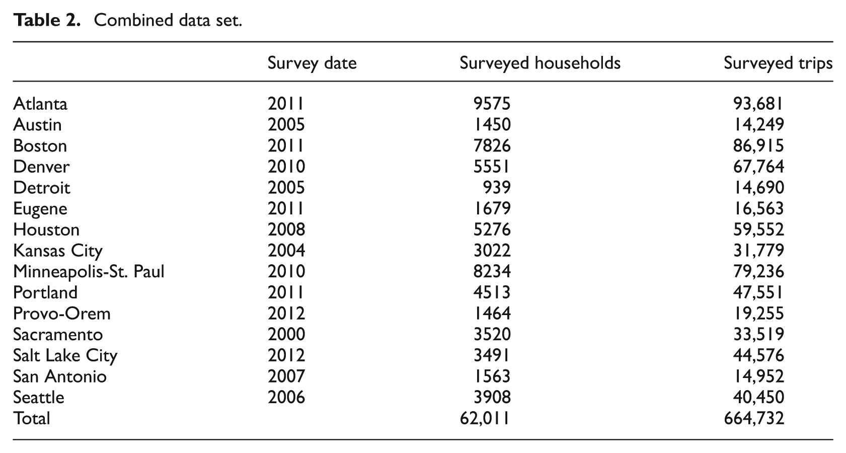
At present, we have consistent data sets for 15 regions. Earlier Atlanta, Boston, Houston and Portland data sets have been dropped for purposes of cross-sectional analysis in favour of newer data sets. The resulting pooled data set consists of 664,732 trips by 62,011 households in the 15 regions (see Table 2). The regions are as diverse as Boston and Portland at one end of the urban form continuum and Houston and Kansas City at the other.

Table 2.

Combined data set.

	Survey date	Surveyed households	Surveyed trips
Atlanta	2011	9575	93,681
Austin	2005	1450	14,249
Boston	2011	7826	86,915
Denver	2010	5551	67,764
Detroit	2005	939	14,690
Eugene	2011	1679	16,563
Houston	2008	5276	59,552
Kansas City	2004	3022	31,779
Minneapolis-St. Paul	2010	8234	79,236
Portland	2011	4513	47,551
Provo-Orem	2012	1464	19,255
Sacramento	2000	3520	33,519
Salt Lake City	2012	3491	44,576
San Antonio	2007	1563	14,952
Seattle	2006	3908	40,450
Total		62,011	664,732

To our knowledge, this is the largest sample of household travel records ever assembled for such a study outside the National Household Travel Survey (NHTS). And relative to NHTS, our data base provides much larger samples for individual regions and permits the calculation of a wide array of built environmental variables based on the precise location of households. NHTS provides geocodes (identifies households) only at the census tract level.

Variables

The dependent and independent variables used in this study are defined in Table 3. Sample sizes and descriptive statistics are also provided. For individual trips, trip purpose, travel mode and travel time are available from the survey data sets. Distance travelled on each trip was either supplied or computed with GIS from the XY coordinates. For travellers, individual age, employment status, race and driver’s licensure are available from the survey data sets. For households, household size, household income and vehicle ownership are available from the survey data sets. This allows us to control for sociodemographic influences on travel at the household level.

Table 3.

Dependent and independent variables.

Variable	Description	N	Mean	S.D.
Dependent variables
anyvmt	any household VMT (1 = yes, 0 = no)	62,011	0.94	0.24
lnvmt	natural log of household VMT (for households with any VMT)	58,011	3.07	1.03
autotrips	household car trips	62,011	8.4	7.11
anywalk	any household walk trips (1 = yes, 0 = no)	62,011	0.24	0.43
walktrips	household walk trips (for households with any walk trips)	14,672	4.08	3.51
anybike	any household bike trips (1 = yes, 0 = no)	62,011	0.04	0.2
biketrips	household bike trips (for households with any bike trips)	2495	3.24	2.63
anytransit	any household transit trips (1 = yes, 0 = no)	62,011	0.11	0.31
transittrips	household transit trips (for households with any transit trips)	6719	2.97	2.22
Independent variables – household
hhsize	household size	62,011	2.54	1.39
hhworkers	number employed	62,011	1.28	0.88
hhincome	real household income(in 1000s of 2012 dollars)	62,011	79.9	51.1
Independent variables – buffers
actdenqtrmi	activity density within one-quarter mile (pop + emp per square mile in 1000s)	62,011	7.24	12.09
jobpopqmi²	job-population balance within one-quarter mile	62,011	0.59	0.26
entropyqmi³	land use entropy within one-quarter mile	62,011	0.22	0.27
intdenqmi	intersection density within one-quarter mile	62,011	172.47	117.25
int4wqmi	percentage 4-way intersections within one-quarter mile	62,011	27.13	26.4
stopdenqmi	transit stop density within one-quarter mile	62,011	26.2	47.25
actdenhmi	activity density within one-half mile (pop + emp per square mile in 1000s)	62,011	7.07	11.59
jobpophmi²	job-population balance within one-half mile	62,011	0.61	0.25
entropyhmi³	land use entropy within one-half mile	62,011	0.36	0.28
intdenhmi	intersection density within one-half mile	62,011	137.96	93.85
int4whmi	percentage 4-way intersections within one-half mile	62,011	26.59	21.14
stopdenhmi	transit stop density within one-half mile	62,011	23.74	33.47
actden1mi	activity density within one mile (pop + emp per square mile in 1000s)	62,011	7.38	10.52
jobpop1mi²	job-population balance within one mile	62,011	0.63	0.25
entropy1mi³	land use entropy within one mile	62,011	0.47	0.26
intden1mi	intersection density within one mile	62,011	118.54	84.78
int4w1mi	percentage 4-way intersections within one mile	62,011	26.31	17.82
stopden1mi	transit stop density within one mile	62,011	21.37	26.47
railhmi	rail station within one-half mile (1 = yes, 0 = no)	62,011	0.08	0.7
emp10a	percentage of regional employment within 10 min by car	62,011	7.49	10.35
emp20a	percentage of regional employment within 20 min by car	62,011	29.21	26.26
emp30a	percentage of regional employment within 30 min by car	62,011	51.3	29.16
emp30t	percentage of regional employment within 30 min by transit	62,011	21.41	21.36
Independent variables – region
regpop	population within the region 1000s	15	2753.92	1690.62
compact	Measure of regional compactness developed by Ewing and Hamidi (2014); higher values of the index correspond to more compact development, lower values to more sprawling development.	15	101.09	26.03

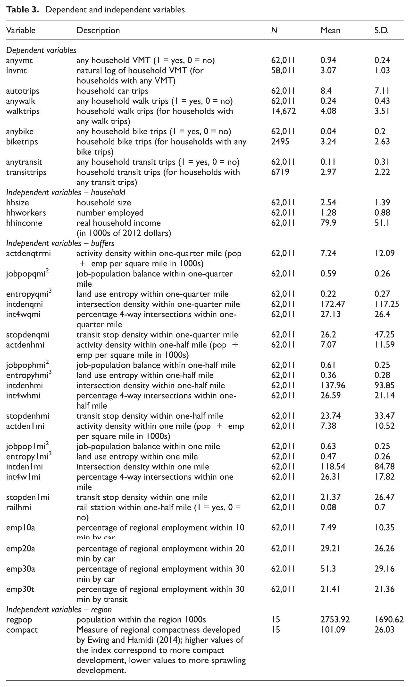
The variables in this study cover all of the Ds, from density to demographics. With different measures and different buffer widths, a total of 26 independent variables are available to explain household travel outcomes. The variables are consistently defined across regions. That is one of the main strengths of this study.

Statistical analysis

To increase statistical power and external validity, we pooled household travel data from 15 diverse regions. Our data and model structure are hierarchical, with households ‘nested’ within regions.

The best statistical approach to nested data is multilevel modelling (MLM), also called hierarchical modelling (HLM). MLM modelling is just beginning to be used in the planning field (Ewing et al., 2011, 2013). MLM accounts for dependence among observations, in this case the dependence of households within a given region on characteristics of the region. All households within a given region share these characteristics. This dependence violates the independence assumption of ordinary least squares (‘OLS’) regression. Standard errors of regression coefficients based on OLS will consequently be underestimated. Moreover, OLS coefficient estimates will be inefficient. MLM overcomes these limitations, accounting for the dependence among observations and producing more accurate coefficient and standard error estimates (Raudenbush and Bryk, 2002).

Regions such as Boston and Houston are likely to generate very different travel patterns regardless of household and neighbourhood characteristics. The essence of MLM is to isolate the variance associated with each data level. MLM partitions variance between the household/neighbourhood level (Level 1) and the region level (Level 2) and then seeks to explain the variance at each level in terms of D variables. We can expect to explain a good portion of the variance at Level 1 given the large number of available variables and the large sample of households. We cannot expect to explain much of the variance at Level 2 with such a small sample of regions. Variables such as regional population (as a measure of region size) may not prove statistically significant predictors of household travel because of limited degrees of freedom. Still, there is a statistical advantage to partitioning the variance as MLM does, and estimating a random effects model. Regional variance is captured in the random effects term of the Level 2 equations.

The dependent variables are of two types: continuous (household VMT) and counts (household car trips, walk trips, bike trips and transit trips). VMT per household has two characteristics that complicate the modelling of it. First, it is non-normally distributed, highly skewed to the right. The solution to this problem is to take the natural logarithm of VMT, which becomes our dependent variable. Second, it has a large number of zero values for households that generate no VMT. These households use only alternative modes such as transit or walking. Six percent of households in the sample fall into this category. When VMT is log transformed, these households have undefined values of the dependent variable.

In the planning literature, the problem of zero values is often handled by adding one (1.0) to the value of a dependent variable and then log transforming the variable. The 1 becomes a 0 when transformed. This is not econometrically correct, however, since households with zero values may be qualitatively different than those with positive values. ‘In some settings, the zero outcome of the data-generating process is qualitatively different from the positive ones. The zero or nonzero values of the outcome is the result of a separate decision whether or not to “participate” in the activity. On deciding to participate, the individual decides separately how much to participate, that is, how intensively [to participate]’ (Greene, 2012: 824).

A solution to the problem of excess zero values (what is referred to in the econometric literature as ‘zero inflation’) is to estimate two-stage ‘hurdle’ models (Greene, 2012: 443, 824–826). The stage 1 model categorises households as either generating VMT or not. The stage 2 model estimates the amount of VMT generated for households with any (positive) VMT. We are aware of no previous application of hurdle models to the planning field.⁴

The other type of variable that we wish to model is trip counts. We have four trip counts among our dependent variables – car, walk, bike and transit trip counts for each household. These also require special treatment. Two basic methods of analysis are available when the dependent variable is a count, with non-negative integer values, many small values and few large ones. The methods are Poisson regression and negative binomial regression.

The two models – Poisson and negative binomial – differ in their assumptions about the distribution of the dependent variable. Negative binomial regression is appropriate if the dependent variable is overdispersed, meaning that the variance of counts is greater than the mean. Popular indicators of overdispersion are the Pearson and χ² statistics divided by the degrees of freedom, so-called dispersion statistics. If these statistics are greater than 1.0, a model is said to be overdispersed (Hilbe, 2011: 88, 142). By these measures, we have overdispersion of trip counts in our data set, and the negative binomial model is more appropriate than the Poisson model.

The other statistical complication is the excess number of zero values for three of the four count variables. The exception is household car trips. Only 6% of households are without car trips. The frequency distribution of car trips follows a negative binomial distribution rather closely, and these can be modelled in a single stage. In contrast, 76% percent of households have no walk trips, 96% have no bike trips and 89% have no transit trips. Again, the solution to the problem of zero inflation is to estimate two-stage hurdle models. The first stage is the estimation of logistic regression models to distinguish between households with and without walk, bike or transit trips. The second stage is the estimation of negative binomial regression models for the number of trips by these modes for households that have such trips.

Results

Models were estimated with HLM 7, Hierarchical Linear and Nonlinear Modeling software (Raudenbush et al., 2010). HLM 7 allows the estimation of multilevel models for continuous, dichotomous and count variables, and for the last of these, HLM 7 can account for overdispersion.

There is no theoretically superior model involving different D variables and different buffer widths. Theoretically, buffers could be wide or narrow. Even a determinant as straightforward as walking distance could be anywhere from one-quarter mile to one mile or more. Different Ds may emerge as significant in different models. So trial and error was used to arrive at the best-fit models for the travel outcomes of interest. Variables were substituted into models to see if they were statistically significant and improved goodness-of-fit. For each dependent variable, we were looking for the model with the most significant t-statistics and the greatest log-likelihood.

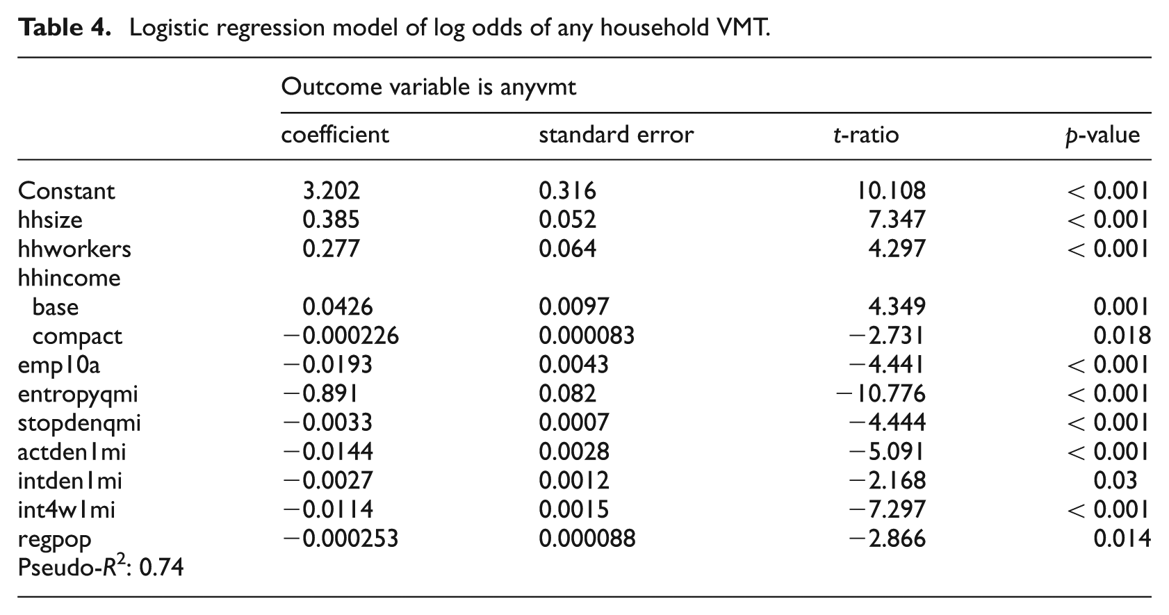
The best-fit model for the dichotomous variable, any VMT (1 = yes, 0 = no), is presented in Table 4. The likelihood of a household generating any VMT increases with household size, number of employed members and real household income. However, the likelihood of any VMT at the mean household income is higher for households from sprawl regions than households from compact regions. The likelihood of any VMT declines with the percentage of regional employment accessible within 10 minutes by automobile, with land use entropy within one-quarter mile of a household, with transit stop density within one-quarter mile, with activity density within a mile, with intersection density within a mile, with percentage of four-way intersections within a mile, and population within the region. Basically, those who live in highly accessible places (characterised by these five D variables) and larger metropolitan areas are better able to make do without car trips. However, the probability of any VMT remains high for all cohorts.

Table 4.

Logistic regression model of log odds of any household VMT.

	Outcome variable is anyvmt
	coefficient	standard error	t-ratio	p-value
Constant	3.202	0.316	10.108	< 0.001
hhsize	0.385	0.052	7.347	< 0.001
hhworkers	0.277	0.064	4.297	< 0.001
hhincome
base	0.0426	0.0097	4.349	0.001
compact	−0.000226	0.000083	−2.731	0.018
emp10a	−0.0193	0.0043	−4.441	< 0.001
entropyqmi	−0.891	0.082	−10.776	< 0.001
stopdenqmi	−0.0033	0.0007	−4.444	< 0.001
actden1mi	−0.0144	0.0028	−5.091	< 0.001
intden1mi	−0.0027	0.0012	−2.168	0.03
int4w1mi	−0.0114	0.0015	−7.297	< 0.001
regpop	−0.000253	0.000088	−2.866	0.014
Pseudo-R²: 0.74

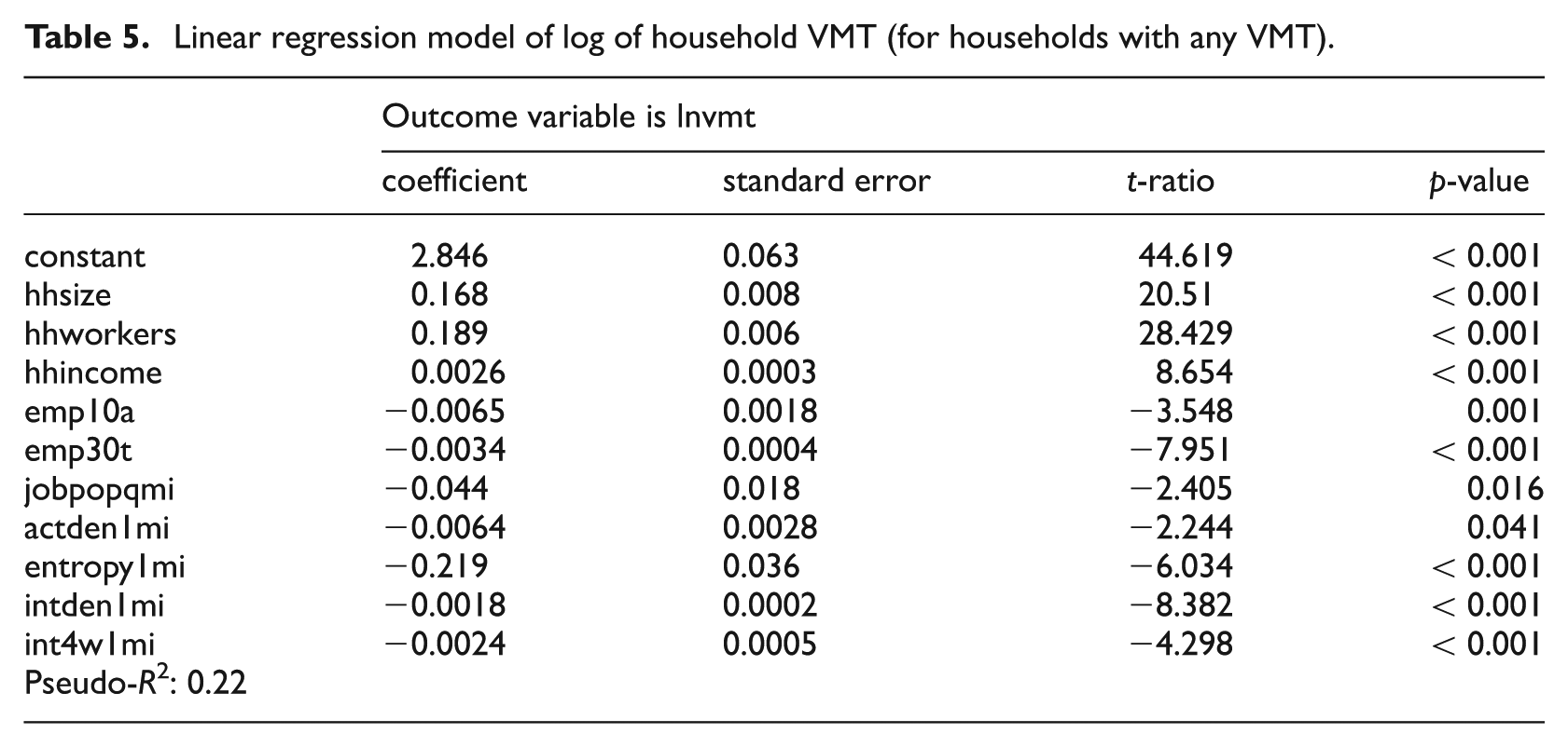
The best-fit model for the continuous variable natural logarithm of VMT (for households that generate VMT) is presented in Table 5. Results parallel those for the dichotomous variable any VMT, though the exact specification of the model is different. Household VMT increases with the household size, number of employed household members and real household income. Household VMT declines with two destination accessibility variables: percentage of regional employment accessible within 10 minutes by automobile and percentage of regional employment accessible within 30 minutes by transit. Household VMT also declines with two land use diversity variables characterising one-quarter-mile and one-mile buffers around households: job–population balance and land use entropy. Finally, household VMT declines with activity density, intersection density and percentage of 4-way intersections within one mile. Again, those who live in highly accessible places (characterised by these D variables) generate less VMT than those in less accessible places.

Table 5.

Linear regression model of log of household VMT (for households with any VMT).

	Outcome variable is lnvmt
	coefficient	standard error	t-ratio	p-value
constant	2.846	0.063	44.619	< 0.001
hhsize	0.168	0.008	20.51	< 0.001
hhworkers	0.189	0.006	28.429	< 0.001
hhincome	0.0026	0.0003	8.654	< 0.001
emp10a	−0.0065	0.0018	−3.548	0.001
emp30t	−0.0034	0.0004	−7.951	< 0.001
jobpopqmi	−0.044	0.018	−2.405	0.016
actden1mi	−0.0064	0.0028	−2.244	0.041
entropy1mi	−0.219	0.036	−6.034	< 0.001
intden1mi	−0.0018	0.0002	−8.382	< 0.001
int4w1mi	−0.0024	0.0005	−4.298	< 0.001
Pseudo-R²: 0.22

The number of household automobile trips increases with household size, number of employed members and real household income (see Table 6). Automobile trip frequency declines with land use entropy within one-quarter mile, activity density within one-half mile, and transit stop density within one-half mile. This kind of trip degeneration is doubtless due to substitution of walk, bike and transit trips for automobile trips when trip destinations and transit stops are nearby, and may also be due to the ability of households to complete multi-purpose trips when destinations are concentrated within a short automobile trip. Automobile trip frequency increases with job–population balance within a mile and with accessibility to employment within 20 minutes by automobile (a proxy for trip attractions). This rise in trip making with enhanced accessibility is predicted by economic theory, since the generalised cost per trip is lower at accessible locations.

Table 6.

Negative binomial model of household automobile trips.

	Outcome variable is autotrips
	coefficient	standard error	t-ratio	p-value
constant	1.289	0.046	27.871	< 0.001
hhsize	0.305	0.009	33.009	< 0.001
hhworkers	0.007	0.004	1.700	0.086
hhincome	0.0015	0.0002	6.812	< 0.001
emp20a	0.00104	0.00028	3.753	< 0.001
entropyqmi	−0.065	0.014	−4.495	< 0.001
actdenhmi	−0.0043	0.0008	−4.934	< 0.001
stopdenhmi	0.0007	0.00016	−4.414	< 0.001
jobpop1mi	0.022	0.012	1.809	0.07
Pseudo-R²: 0.52

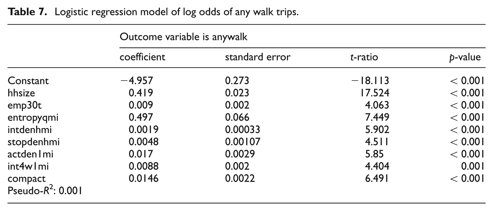
Our walk trip models conform to theory. The likelihood of a household making any walk trips increases with household size (see Table 7). The likelihood of any walk trips increases with land use entropy within one-quarter mile of home, intersection density within one-half mile of home, and activity density and percentage of 4-way intersections within a mile of home. These measures of density, diversity and design place destinations within walking distance of home. The likelihood of any walk trips also increases with accessibility to employment within 30 minutes by transit and with transit stop density within one-half mile of home. Transit service is complementary to walking, as households with good access to transit tend to own fewer automobiles, having transit available for their work trips. Owning fewer automobiles, they are more likely to walk on their non-work trips. The likelihood of any walk trips also increases with regional compactness. The more compact a region is, the more destinations are within a walkable distance.

Table 7.

Logistic regression model of log odds of any walk trips.

	Outcome variable is anywalk
	coefficient	standard error	t-ratio	p-value
Constant	−4.957	0.273	−18.113	< 0.001
hhsize	0.419	0.023	17.524	< 0.001
emp30t	0.009	0.002	4.063	< 0.001
entropyqmi	0.497	0.066	7.449	< 0.001
intdenhmi	0.0019	0.00033	5.902	< 0.001
stopdenhmi	0.0048	0.00107	4.511	< 0.001
actden1mi	0.017	0.0029	5.85	< 0.001
int4w1mi	0.0088	0.002	4.404	0.001
compact	0.0146	0.0022	6.491	< 0.001
Pseudo-R²: 0.001

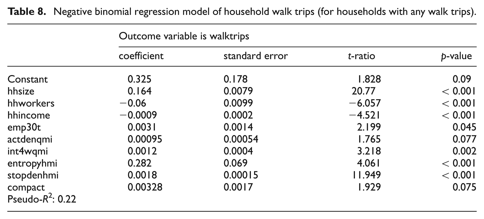
The number of walk trips for the subset of households that make walk trips increases with household size and declines with household income and number of employed members (see Table 8). The last of these relationships is counterintuitive but actually makes sense. The overwhelming majority of walk trips are for non-work purposes. Workers are otherwise engaged rather than walking during the workday. The number of walk trips increases with these D variables: activity density within one-quarter mile, percentage of 4-way intersections within one-quarter mile, and land use entropy within one-half mile of home. It also increases with transit accessibility to employment within 30 minutes, transit stop density within one-half mile of home and regional compactness. The relationship of walking to density, diversity and design has already been discussed, as has the relationship of walking to transit service and regional compactness. Probably the most interesting finding is that walk trip frequency depends on the built environment at a larger scale than the usual one-quarter mile walk distance assumed by planners. In fact, according to the Nationwide Household Travel Survey (NHTS), the average walk trip length in the USA varies by trip purpose from 0.52 miles for shopping trips to 0.88 miles for work trips. The overall average is 0.70 miles, which implies a relevant environmental scale of one-half to one mile.

Table 8.

Negative binomial regression model of household walk trips (for households with any walk trips).

	Outcome variable is walktrips
	coefficient	standard error	t-ratio	p-value
Constant	0.325	0.178	1.828	0.09
hhsize	0.164	0.0079	20.77	< 0.001
hhworkers	−0.06	0.0099	−6.057	< 0.001
hhincome	−0.0009	0.0002	−4.521	< 0.001
emp30t	0.0031	0.0014	2.199	0.045
actdenqmi	0.00095	0.00054	1.765	0.077
int4wqmi	0.0012	0.0004	3.218	0.002
entropyhmi	0.282	0.069	4.061	< 0.001
stopdenhmi	0.0018	0.00015	11.949	< 0.001
compact	0.00328	0.0017	1.929	0.075
Pseudo-R²: 0.22

The likelihood of a household making any bike trips depends on household size and number of workers (see Table 9). Both of the two have a positive relationship. It also depends on diversity and design variables, specifically with job–population balance within one-half mile of home, intersection density and percentage of 4-way intersections within a mile of home. Regional compactness is also significant, suggesting that compact regions encourage bike trips. Relationships do not appear to be as strong for bicycling as for walking.

Table 9.

Logistic regression model of log odds of any bike trips.

	Outcome variable is anybike
	coefficient	standard error	t-ratio	p-value
Constant	−6.689	0.52	−12.861	< 0.001
hhsize	0.386	0.03	12.89	< 0.001
hhworkers	0.181	0.044	4.072	< 0.001
jobpophmi	0.362	0.102	3.552	0.001
intden1mi	0.0032	0.0017	1.911	0.076
int4w1mi	0.0158	0.005	3.127	0.008
compact	0.01	0.005	1.752	0.103
Pseudo-R²: NA

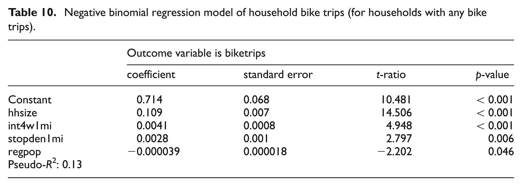
Bike trip frequency for the subset of households that make bike trips increases with household size, increases with the percentage of 4-way intersections within a mile, increases with transit stop density within a mile, and declines with regional population (see Table 10). The second of these relationships suggests the importance of an interconnected street network as a facilitator of biking, perhaps because it shortens trip distances or provides routing options. It may simply mean that bicyclists are not channelled up and down the suburban hierarchy of streets and therefore can avoid high speed arterials. The third of these relationships may be explained by the same phenomena as with walking. Bicycle use may be complementary to transit use. The fourth of these relationships suggests that big regions make biking to destinations less feasible. This is the only model that we might describe as underspecified. Other variables may prove significant as our sample of households with bike trips expands with the addition of other regions. The current sample, 2495 households with bike trips, is our smallest.

Table 10.

Negative binomial regression model of household bike trips (for households with any bike trips).

	Outcome variable is biketrips
	coefficient	standard error	t-ratio	p-value
Constant	0.714	0.068	10.481	< 0.001
hhsize	0.109	0.007	14.506	< 0.001
int4w1mi	0.0041	0.0008	4.948	< 0.001
stopden1mi	0.0028	0.001	2.797	0.006
regpop	−0.000039	0.000018	−2.202	0.046
Pseudo-R²: 0.13

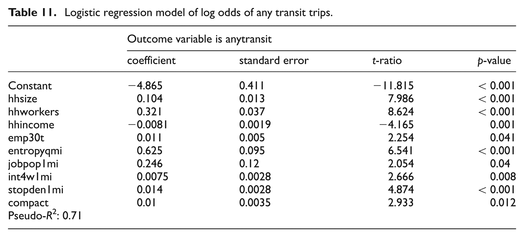
The likelihood of a household having any transit trips increases with household size and number of employed members, and declines with income (see Table 11). It also depends on diversity and design of the environment around a household, and regional compactness. Transit-oriented development is virtually defined by these variables. The most relevant environmental scale is one mile. This might suggest longer transit access trips than the transit industries’ rule of thumb, one-quarter mile. Or it might simply reflect the complementary nature of walking, biking and transit use. Two transit service variables affect the likelihood of transit trips: percentage of regional jobs that can be reached by transit in 30 minutes and transit stop density within a mile of home.

Table 11.

Logistic regression model of log odds of any transit trips.

	Outcome variable is anytransit
	coefficient	standard error	t-ratio	p-value
Constant	−4.865	0.411	−11.815	< 0.001
hhsize	0.104	0.013	7.986	< 0.001
hhworkers	0.321	0.037	8.624	< 0.001
hhincome	−0.0081	0.0019	−4.165	0.001
emp30t	0.011	0.005	2.254	0.041
entropyqmi	0.625	0.095	6.541	< 0.001
jobpop1mi	0.246	0.12	2.054	0.04
int4w1mi	0.0075	0.0028	2.666	0.008
stopden1mi	0.014	0.0028	4.874	< 0.001
compact	0.01	0.0035	2.933	0.012
Pseudo-R²: 0.71

The number of household transit trips for the subset of households that use transit increases with household size, and declines with employment and household income (see Table 12). Transit trip frequency increases with percentage of regional jobs that can be reached by transit in 30 minutes and transit stop density within one-quarter mile of home, two transit service variables. Transit trip frequency also increases with land use entropy within one-half mile and job–population balance within a mile of home, two measures of land use mix. It has long been speculated that mixed-use areas would generate more transit trips because the feasibility of trip chaining on the access trip to transit, that is, stopping along the way to conduct other personal business. Transit trip frequency also increases with regional population. Large metropolitan areas have better transit service.

Table 12.

Negative binomial regression model of household transit trips.

	Outcome variable is transittrips
	coefficient	standard error	t-ratio	p-value
Constant	0.525	0.124	4.236	0.001
hhsize	0.092	0.02	4.538	< 0.001
hhworkers	−0.018	0.008	−2.203	0.028
hhincome	−0.0027	0.0002	−13.515	< 0.001
emp30t	0.0021	0.0008	2.533	0.012
stopdenqmi	0.00048	0.00011	4.345	< 0.001
entropyhmi	0.188	0.053	3.512	0.001
jobpop1mi	0.187	0.086	2.182	0.029
regpop	0.000066	0.000032	2.064	0.059
Pseudo-R²: 0.17

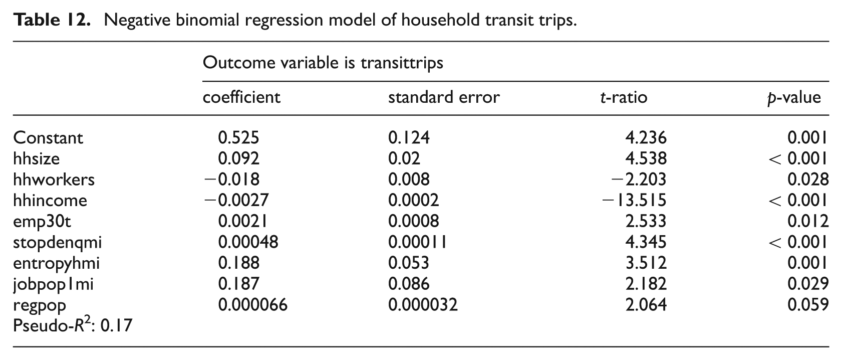
Shown are pseudo-R²s, largely because urban planners are used to dealing with R²s and may want this information. Pseudo-R²s in multilevel modelling are not equivalent to R²s in ordinary least squares regression, and should not be interpreted the same way. The pseudo-R² bears some resemblance to the statistic used to test the hypothesis that all coefficients in the model are zero, but there is no construction by which it is a measure of how well the model predicts the outcome variable in the way that R² does in conventional regression analysis.

Discussion

Generalising across the preceding models, four conclusions emerge with great relevance to travel modelling:

Socioeconomic, built environment and transit service variables all influence household travel decisions, though based on the significance levels alone, the socioeconomic influences appear strongest.

The decision to use alternative modes is influenced by different factors than the frequency of use once the decision is made, and the use of hurdle models is therefore warranted in household travel modelling.

All the D variables influence household travel decisions, but consistent with the meta-analysis by Ewing and Cervero (2010), the strongest influences are diversity, design and destination accessibility, and the weakest influence in a multivariate context is density.

The relevant built environment for travel analysis is anywhere from one-quarter to one mile or more in scale, but the largest scale seems have more predictive power than the smallest scale.

A number of caveats apply to these results. First, the sample for this study, while large in terms of households, covers only 15 regions of the USA. Thus for certain outcome variables, we are unable to predict variations in household travel behaviour across regions. As the sample of regions expands, so will the external validity of the study and our ability to predict variations.

Second, this study focuses exclusively on the home end of trips, when every trip has two ends. We set out to measure environmental conditions at all origins and destinations, but discovered that the analytical requirements exceeded the capacity of our software and hardware, given our large sample of trips. Some variables that are included in our models, such as percentage of regional employment accessible within a 30 minute travel time by car, at least account for more than simple neighbourhood effects.

Third, the list of predictor variables, while longer than any previous study’s, still omits certain variables that have presumptive effects on household travel. Among the D variables, design characteristics such as sidewalk coverage and building setbacks are unavailable in large data sets. Also missing are variables related to another D, demand management. Parking supplies and prices, particularly at the destination end of trips, may strongly affect mode choices of workers.

Finally, we cannot draw strong causal inferences from a cross-sectional study such as this one. The main threat to causal inference is self-selection, where individuals who want to walk, bike or use transit choose to live in walkable, bikeable or transit-served neighbourhoods. These individuals would be inclined to use active modes of travel wherever they lived. We have no ability to control for such effects in this multi-region study, as most of the underlying household surveys do not include relevant attitudinal questions. This caveat may not be as important as one might think. Nearly all studies of residential self-selection have found ‘resounding’ evidence of statistically significant associations between the built environment and travel behaviour, independent of self-selection influences (Cao et al., 2009a: 389). Where the magnitude of the self-selection effect has been compared with the effect of the built environment on travel, the former has been found to be secondary.⁵ There may be good explanations for this unexpected result. In a region with few pedestrian-, bike-, and transit-friendly neighbourhoods, residential self-selection likely matches individual preferences with place characteristics, increasing the effect of the D variables, a possibility posited by Lund et al. (2006) and Chatman (2009).

Computations

The models developed in this study give us natural logarithms, log odds, and expected values of variables. Model outputs must be transformed to compute effects. The transformations involve several steps.

For example, for transit trips, the logistic equation in Table 11 allows us to compute the odds of any transit trips by exponentiating the log odds, and then to compute the probability of any transit trips with the formula for the probability in terms of the odds.

\begin{matrix} odds of any transit trips \\ = \exp (log odds any transit trips) \end{matrix}

(1)

\begin{matrix} probability of any transit trips \\ = odds of any transit trips / \\ (1 + odds of any transit trips) \end{matrix}

(2)

From the negative binomial equation in Table 12, we next compute the expected number of transit trips for households with any transit trips, again, by exponentiating:

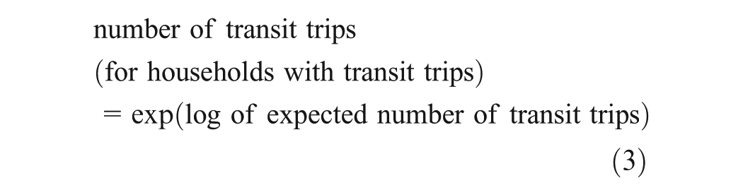
\begin{matrix} number of transit trips \\ (for households with transit trips) \\ = \exp (log of expected number of transit trips) \end{matrix}

(3)

The expected number of transit trips for all households is just the product of the two.

\begin{matrix} number of transit trips (for all households) \\ = probability of any transit trips \\ \times number of transit trips \\ (for households with transit trips) \end{matrix}

(4)

Predicting VMT is trickier. When the regression model is fit in logs, the prediction for the log of the dependent variable is exponentiated to predict the variable itself. But, this method predicts the median of the dependent variable, not the mean. To obtain a prediction of the mean, the exponentiated variable is multiplied by a factor equal to exp(s-squared / 2) where s-squared is the standard error of the regression (i.e. the standard deviation of the residuals) for the loglinear model. The scale factor in this case is estimated to be 1.505. Another scale factor is required to convert from minimum network distance between origin and destination, used to compute VMT, and actual roadway distance between origin and destination. That scale factor is estimated to be 1.36.

Applications

The models developed in this study have already been incorporated into Envision Tomorrow Plus (ET+), a leading scenario planning software package developed by Fregonese Associates of Portland, OR. This software is user-friendly, transparent and open source. The software is currently being used in Austin, TX, Cleveland, OH, Kansas City, KS, Salt Lake City, UT, San Diego, CA and other metropolitan regions.

The models have many potential applications. Most obviously, they can be used to post-process outputs of conventional four-step travel demand models. Four-step models are patently inadequate when it comes to accounting for density, diversity and design effects on household travel. They treat all development as if located at the centroids of traffic analysis zones, and local street networks as if completely represented by two or three centroid connectors to the external street network. Thus they cannot distinguish between dense, mixed, interconnected development and sprawling single-use development with the same housing and employment totals. They fail to account for the effects of accessibility on trip generation rates. They use crude approximations to predict intrazonal travel. They typically ignore the effects of density, diversity and design on mode choice.

The literature covers post-processing applications well (Cervero, 2006; DKS Associates, 2007; Johnston, 2004; Walters et al., 2000). These new models can be used in exactly the same way as earlier elasticity estimates from the literature, which have found their way into regional transportation planning.

Sketch planning applications of the models are limited only by the creativity of planning analysts. To illustrate, climate action planning of the type currently underway in California, Oregon, and 17 other states will require VMT estimates in order to extrapolate current trends and project an alternative lower-carbon future. These states have set greenhouse gas emission reduction targets and, with their metropolitan planning organisations, will need to pull together verifiable plans that include smart-growth elements. If planners are willing to make assumptions about the increases in density and other D variables that can be achieved with policy changes, they can use models in this article to estimate VMT reductions in urbanised areas, and to translate these in turn into CO₂ reductions.

Another potential sketch planning application could be to assess health impacts of development. Rates of physical activity, including walking and biking, are inputs to health assessment models. Again, once planners make assumptions about changes in the D variables under future scenarios, increases in walking and biking can easily be computed using the models above. Until now there has been no empirically grounded methodology for making such projections for bicycle use.

Models could also be applied to traffic impact analysis. There has been no way to adjust the Institute of Transportation Engineers’ (ITE) trip generation rates for walking, biking and transit use, which has left developers of dense developments at urban sites paying impact fees and other exactions at the same rate as their suburban counterparts. The only adjustment previously allowed was for internal capture of trips within mixed-use developments, which did nothing for the typical infill project. Models can be used to adjust ITE trip rates, which are derived from car-oriented suburban developments, to reflect how greater densities and other environmental attributes would affect trip making.

It is our hope that models introduced herein will find wide application in the planning field.

Footnotes

Funding

Funding was received from a HUD Sustainable Communities Grant.

Notes

References

Ben-Akiva

Lerman

(1985) Discrete Choice Analysis. Cambridge, MA: MIT Press.

Bhat

Sen

Eluru

(2009) The impact of demographics, built environment attributes, vehicle characteristics, and gasoline prices on household vehicle holdings and use. Transportation Research Part B 43(1): 1–18.

Boarnet

Crane

(2001) The influence of land use on travel behavior: Specification and estimation strategies. Transportation Research A 35(9): 823–845.

Brownstone

(2008) Key Relationships Between the Built Environment and VMT. Special Report 298: Driving and the Built Environment. Washington, DC: Transportation Research Board.

Cao

(2010) Exploring causal effects of neighborhood type on walking behavior using stratification on the propensity score. Environment and Planning A 42(2): 487–504.

Cao

Mokhtarian

Handy

(2009a) Examining the impacts of residential self-selection on travel behavior: A focus on empirical findings. Transport Reviews 29(3): 359–395.

Cao

Mokhtarian

Handy

(2009b) The relationship between the built environment and nonwork travel: A case study of northern California. Transportation Research A 43(5): 548–559.

Cao

Fan

(2009c) Exploring the connections among residential location, self-selection, and driving behavior: A case study of Raleigh, NC. Paper presented at the 89th annual meeting of the Transportation Research Board.

Cervero

(2002) Built environments and mode choice: Toward a normative framework. Transportation Research D 7(4): 265–284.

10.

Cervero

(2006) Alternative approaches to modeling the travel-demand impacts of smart growth. Journal of the American Planning Association 72(3): 285–295.

11.

Cervero

Kockelman

(1997) Travel demand and the 3Ds: Density, diversity, and design. Transportation Research D 2(3): 199–219.

12.

Chatman

(2009) Residential self-selection, the built environment, and nonwork travel: Evidence using new data and methods. Environment and Planning A 41(5): 1072–1089.

13.

Crane

(1996) On form versus function: Will the new urbanism reduce traffic, or increase it? Journal of Planning Education and Research 15(2): 117–126.

14.

DKS Associates (2007) Assessment of Local Models and Tools for Analyzing Smart-Growth Strategies: Final Report. Sacramento, CA: California Department of Transportation.

15.

Domencich

McFadden

(1975) Urban Travel Demand: A Behavioral Analysis. Amsterdam: North-Holland.

16.

Ewing

Cervero

(2001) Travel and the built environment. Transportation Research Record 1780: 87–114.

17.

Ewing

Cervero

(2010) Travel and the built environment: A meta-analysis. Journal of the American Planning Association 76(3): 265–294.

18.

Ewing

Hamidi

(2014) Measuring Sprawl and Validating Sprawl Measures. Washington, DC: Smart Growth America/USEPA.

19.

Ewing

Greenwald

Zhang

. (2011) Traffic generated by mixed-use developments – A six-region study using consistent built environmental measures. Journal of the Urban Planning and Development 137(3): 248–261.

20.

Ewing

Bogaerts

Zhang

. (2013) Predicting transportation outcomes for LEED-ND pilot projects. Journal of Planning Education and Research 33(3): 265–279.

21.

Greene

(2012) Econometric Analysis. New York: Prentice Hall.

22.

Greenwald

(2003) The road less traveled: New urbanist inducements to travel mode substitution for non-work trips. Journal of Planning Education and Research 23(1): 39–57.

23.

Greenwald

McNally

(2008) Testing land use influences on trip chaining behavior in Portland, Oregon. Proceedings of the Institute for Civil Engineers – Urban Design and Planning (United Kingdom) 161: 61–74.

24.

Hilbe

(2011) Negative Binomial Regression. Cambridge: Cambridge University Press.

25.

Johnston

(2004) The urban transportation planning process. In: Hanson

Guiliano

(eds) The Geography of Urban Transportation. New York, NY: Guilford Press, pp. 115–140.

26.

Kockelman

(1997) Travel behavior as a function of accessibility, land use mixing, and land use balance: Evidence from the San Francisco Bay Area. Transportation Research Record 1607: 116–125.

27.

Lund

Willson

Cervero

(2006) A re-evaluation of travel behavior in California TODs. Journal of Architectural and Planning Research 23(3): 247–263.

28.

Pont

Ziviani

Wadley

. (2009) Environmental correlates of children’s active transportation: A systematic literature review. Health & Place 15(3): 827–840.

29.

Raudenbush

Bryk

(2002) Hierarchical Linear Models: Applications and Data Analysis Methods. 2nd edition. Thousand Oaks, CA: Sage Publications.

30.

Raudenbush

Bryk

Cheong

. (2010) HLM 7: Hierarchical Linear and Nonlinear Modeling. Chicago, IL: Scientific Software International.

31.

Salon

(2006) Cars and the City: An Investigation of Transportation and Residential Location Choices in New York City. Davis, CA: Agricultural and Resource Economics, University of California, Davis.

32.

Salon

Boarnet

Handy

. (2012) How do local actions affect VMT? A critical review of the empirical evidence. Transportation Research D 17(7): 495–508.

33.

Walters

Ewing

Allen

(2000) Adjusting computer modeling tools to capture effects of smart growth. Transportation Research Record 1722: 17–26.

34.

Zhang

(2004) The role of land use in travel mode choice: Evidence from Boston and Hong Kong. Journal of the American Planning Association 70(3): 344–361.

35.

Zhou

Kockelman

(2008) Self-selection in home choice: Use of treatment effects in evaluating relationship between built environment and travel behavior. Transportation Research Record 2077: 54–61.