The impacts of urban pricing on social and spatial inequalities: The case study of Lyon (France)

Abstract

With the aim of making a city sustainable, this paper evaluates the impact of setting up urban toll on inequalities. We use several indicators (Gini, Theil and Atkinson indices) to measure changes in the concentration of incomes and gravity-based accessibility. In the case of the Lyon Metropolitan Area (France), we simulate a cordon pricing and evaluate its impacts on inequalities. We adopt a comparison-based approach to reduce the bias resulting from the spatial division. In agreement with the literature, we show that different inequality indicators produce contrasted and sometimes contradictory results, both at the scale of zones or metropolitan level. Results from Theil and Atkinson indicators point out introducing a toll can reduce inequalities in the most peripheral zones. Although we observe an accessibility improvement, particularly for central zones, the first ring (adjacent to the toll zone) is the most adversely affected by toll.

Keywords

gravity-based accessibility social inequalities spatial inequalities urban road pricing

Introduction

The city of the 21st century is faced with the complex and uncertain challenge of sustainability. Sustainability involves the quest for cities that are more environmentally friendly. However, the improvement in the quality of life which, it is assumed, will result from this for all or part of the population, must not be achieved at the cost of increased inequalities. In these circumstances, it has become crucial to measure the impact on inequalities of new policies intended to make cities more sustainable.

One possible way of improving transport sustainability is to implement urban road pricing (Rotaris et al., 2010). Although road pricing is authorised by French legislation,¹ its proven positive effects in terms of reducing road traffic nonetheless mask its significant impacts on inequalities. A measure which increases social inequalities is considered to be regressive as it favours persons with a high value-of-time (VOT) who usually belong to the highest income bracket (Eliasson, 2009; Evans, 1992; Giuliano, 1992; Glazer, 1981; Richardson, 1974). It is also considered to be regressive if it increases geographic inequalities by raising the cost of peripheral localisation (Eliasson and Mattsson, 2006; Raux and Souche, 2004; Rietveld and Verhoef, 1998).

Typically, the impact of a toll on wellbeing is evaluated by the variation of the surplus that it generates (Mayeres and Proost, 2001; Mun and Ahn, 2008; Ramjerdi, 2006; Rouwendal and Verhoef, 2006; Santos and Rojey, 2004; Sumalee et al., 2005). Although it is rarely dealt with in the literature, this variation of surplus can be measured by the variation of inequality indicators related to the concentration of income and accessibility. In spite of its being one of the best-known indicators,² the Gini coefficient of inequality is little used in the literature on urban road pricing (Karlström and Franklin, 2009; Ramjerdi, 2006; Sumalee et al., 2005), and the Theil (Condeço-Melhorado et al., 2011) and Atkinson indices have only been used by Ramjerdi (2006). The variation of gravity-based potential is used classically to measure accessibility (Geurs and van Wee, 2004; Hansen, 1959; Morris et al., 1978). But here again, there are very few studies in the literature that evaluate the impact of urban road pricing on inequalities of access. Although this was done by Condeço-Melhorado et al. (2011), their aim was to simulate the impact of a toll infrastructure on Spanish road and motorway traffic. Above all, Ramjerdi’s (2006) study identified the precautions required to reduce the results’ sensitivity to the level of spatial division.³ In this paper, we free ourselves from this constraint by adopting a comparison-based approach. In this case, the level of spatial division is fixed and higher interest is focused on indicators’ variation rather than its magnitude. Obviously, it is precisely this magnitude which is highly sensitive to the selected level of division.

This paper seeks to evaluate, a priori, the impact of urban road pricing on inequalities. Its originality lies in the use of several indicators of inequality (for example Gini, Theil and Atkinson indices) to measure changes in the concentration of incomes and gravity-based accessibility. In the case of the Lyon Metropolitan Area (France), we have simulated a new pricing measure (an urban road pricing around the Central Business District, e.g. a cordon pricing) and evaluated its impacts on inequalities in comparison with the current situation which is used as a benchmark.

In conformity with the literature, we have found that different indicators of inequality produce contrasted and sometimes contradictory results, both at the scale of zones or of metropolitan area. This result provides evidence against using only one indicator for measuring inequalities and for conducting analyses by zone. Only the Theil and Atkinson indicators show that introducing a toll can reduce inequalities in the most peripheral zones. Although we observe an improvement of accessibility, particularly for central zones, the first ring (adjacent to the toll zone) is the most adversely affected by toll. Our work is structured in three parts. After a review of the literature on the measurement of inequalities, we shall present our method and data, then simulate the implementation of cordon pricing, and evaluate its impact on inequalities.

Review of the literature on the measurement of inequalities

We first present the literature on the measurement of inequalities and after we will define the three inequality indicators.

Measuring social inequalities with specific indicators

The use of specific inequality indicators to measure the effects of a new urban road pricing policy is rarely dealt with in the literature. Apart from the study by Ramjerdi (2006), the other research only uses the Gini index to assess the impact of urban tolls on inequalities (Karlström and Franklin, 2009; Sumalee et al., 2005).

Ramjerdi (2006) underlines the methodological importance of three points: the choice of the unit and variable selected to measure inequality and the very high sensitivity of the indicators to the selected level of spatial division. In particular, the higher the Gini coefficient and the lower the number of classes, the higher the risk of underestimating inequality linked to grouping observations into classes. Since different measures of justice provide different classifications of income distributions, she recommends using several inequality indicators and not studying the justice associated with a specific value of these indicators.

Sumalee et al. (2005) and Karlström and Franklin (2009) use the Gini index to measure the impact of an urban toll on inequalities. Sumalee et al. (2005) identify the localisation and optimal pricing level of a toll zone system. They identify the variation of wellbeing for each origin-destination pair and measure the Gini coefficient which varies from 0.2 (with an outer boundary) to 0.48 (the optimal double boundary scheme). In this way they show that the double boundary type zone is the worst in terms of inequalities. Karlström and Franklin (2009) show that the social inequity of the toll, expressed by the increase of the Gini index, is higher than the differences linked to gender. The possibility of modulating one’s departure times seems to benefit those individuals that have the highest incomes since they can take advantage of more flexible working hours.

Condeço-Melhorado et al. (2011) use the Gini and Theil indicators, but deal with interurban pricing. Their results are differentiated according to the region, underlining the need to conduct analysis by geographic area and consider the impact of a charging policy on spatial cohesion.

To conclude, combining the Gini indicator with other indicators induces a better understanding of inequalities. However, combining several inequality indicators is quite unusual in the literature on urban toll impact. Hence, conducting a more detailed analysis of inequalities is quite novel.

Measuring spatial inequalities using a gravity-based accessibility indicator

By associating the factors of ‘transport’ and ‘activity location’, accessibility reflects the spatial organisation and quality of the transport system available to individuals in order to participate in activities located in different parts of an area (Geurs and van Wee, 2004).

Although a great deal of literature exists on accessibility at the national and regional scales (among them, Geurs and van Wee, 2004; Hou and Li, 2011; Reggiani et al., 2011a; Spence and Linneker, 1994), research into accessibility in urban zones is scarcer (Baht et al., 2000; Grengs, 2010; Holl, 2007; Iacono et al., 2010; Koenig, 1980; Kwan and Weber, 2008; Raux et al., 2008) and, with the exception of Ramjerdi (2006) and Tillema et al. (2011), none measure the consequences of urban road pricing on accessibility. The papers mentioned above highlight the difficulty of conducting a study in an urban environment. Indeed, this scale of analysis influences the three components of accessibility which are monetary costs, temporal costs and the number of available opportunities. First, activities must be precisely localised, perhaps using geolocalisation, because of the division of the city into different zones or districts. The estimation of monetary costs will be closer to reality the more precise the estimation of the distance to be travelled to reach an opportunity (Iacono et al., 2010). Likewise, the heterogeneity of transport supply must be transcribed within the different districts (Holl, 2007). Lastly, spatial division should localise activities at an appropriate scale that can be varied according to the type of opportunities in question (Kwan and Weber, 2008). Following Handy (1992, 1993), Handy and Niemeier (1997), Limanond and Niemeier (2003), Kwan and Weber (2008: 112) underline: ‘an important approach to date has been to measure access to neighbourhood retail and grocery stores (local or neighbourhood accessibility) separately from major employment centres and large shopping centres (regional accessibility)’. Because of higher concentration of jobs than retail, job accessibility is analysed at the scale of a municipality, whereas retail accessibility is considered more at the scale of a neighbourhood. Despite a general reduction in the level of accessibility resulting from the toll, the results are affected by the size of the zones.

Under these circumstances, it is advisable to measure accessibility by considering the smallest possible scale of zoning. It is also necessary to use a precise representation of transport supply to avoid approximations whose impact on the results could be crucial.

Methodology and data

We shall now present the inequality indicators, data and simulation method we used in our case study of Lyon.

Social inequality indicators

Following the literature review, it is necessary to use and compare several inequality indicators. We have therefore chosen to compare the results given by the Gini, Theil and Atkinson indicators using income as the variable. Spatial inequality is measured by a gravity-based accessibility indicator. The before/after comparison reduces the risk of a bias resulting from the choice of scale as it is the same in both situations.

We have made the choice of only three indices (Gini, Theil and Atkinson) among several, especially because they are the main indicators used in the literature. Gini index seems to be the most used to measure inequalities (Almas et al., 2011; Cowel, 2000). These three indicators satisfy all the properties of the inequality index (Chakravarty, 1999; Duro, 2012; Shorrocks, 1980). The properties of a measure of inequality are the following:

The transfer principle of Pigou-Dalton (the inequality measure varies with transfers made in the distribution)

The principle of population of Dalton (the inequality measure is independent from the size of the population)

The symmetry or anonymity axiom (individuals are judged only on their income)

Normalisation (the inequality index takes the zero value for equal distributions)

The translation invariance (if we multiply the income by a constant, the inequality measure does not change).

Second, these three indicators belong to the three categories identified by Chakravarty (1996) for an appropriate inequalities measurement: those based on deviations (such as Gini), those based on entropy or information theory (such as Theil), those based on normative social welfare (such as Atkinson). Chakravarty (1996) identifies a fourth category with indicators based on combinatorics or on the mathematics of probability distributions (such as Hirschman-Herfindahl Index or the index of concentration). However, in this paper, we integrate this category into the first one. First, because this last category can also means concentration indicator such as Gini. Second, as Amiel and Cowel explain (1992: 14), the Herfindhal Index does not respect all the properties of inequality and particularly this index varies under replication of the population.⁴

The Gini coefficient is an income concentration indicator (Gini, 1921). It measures the dispersion of income in the population and the extent to which a policy is progressive or regressive.⁵ For the distribution of income in a population of N individuals, if i = 1,…,n, y_i is the income of individual i, y_j the income of the individual j and µ is the mean income, the Gini coefficient, denoted by G, is written as follows:

G = \frac{1}{2 N^{2} μ} \sum_{i} \sum_{j} | y_{i} - y_{j} |

(1)

This index gives the same weight to inequalities between the poor or the rich. However, it is sensitive to the level of spatial division. Grouping the data into a small number of groups causes a more important downward bias (Deltas, 2003; Lerman and Yitzhaki, 1989; Wodon and Yitzhaki, 2003). Furthermore, the Gini coefficient can be biased by very small samples but is less sensitive to contamination in high incomes than the Theil indicator (Cowell and Flachaire, 2007). Without any decomposition (Dagum, 1980), income is the only parameter taken into account by the Gini index. However, as shown by recent works in the transport field, even if income is the only parameter used, the poorest of the population (categories under social exclusion) cannot be analysed and well understood (Bonsall and Kelly, 2005; Church et al., 2000; Jones and Lucas, 2012).

The Theil index measures the difference between a group’s size in the population and its share of total income⁶ (Theil, 1967). It has a positive value when a group’s income is higher than the mean for all population and a negative value when it is lower. In these circumstances, the change in the indicator following a transfer from a ‘rich’ person to a ‘poor’ person is expressed by a negative change in the indicator. The Theil index, noted T, is written as follows:

T = \log (N) - \sum_{i = 1}^{N} Y_{i} \log (\frac{1}{Y_{i}})

(2)

where N is the number of individuals and Y_i is the share of total income received by individual i. By definition, the upper limit, log(N), is a function of N (the higher the population, the greater the inequality). At the individual level, the equation can be written as follows:

T = \frac{1}{N} \sum \frac{y_{i}}{μ} \log \frac{y_{i}}{μ}

(3)

where y_i is the income of the individual belonging to a population of N individuals and µ is the mean income. With the Theil index is not possible to use negative values because the logarithm induces non-null value. Cowell and Flachaire (2007) show that Theil index is sensitive to extrema values. However, it is more sensitive to changes in high income groups and to income transfers from the poor to the rich.

The Atkinson index adds an ethical judgement made by society to the evaluation of inequalities (Atkinson, 1970). It reveals the value judgements that are made when the parameters of the social wellbeing function are chosen. Atkinson’s social wellbeing index, denoted by AT, is written as:

AT = 1 - {[\sum_{i} (\frac{n_{i}}{N}) {(\frac{y_{i}}{μ})}^{1 - ε}]}^{\frac{1}{(1 - ε)}}

(4)

where N is the number of individuals, n_i the number of individuals in each income category i = 1,…,n, and y_i is income of individual i, µ is the mean income, ε≥ 0 is a parameter that defines the relative aversion to inequality. The Atkinson index is very sensitive to the choice of the parameter ε. When ε = 0 there is no aversion to inequality and when ε tends to infinity the index only considers the poorest observation. When ε increases then the aversion to inequality increase too. When ε = 1, each individual in the population has the same weight. When AT = 0, all the incomes are equal, when AT = 1 one income is null. A transfer from a rich person to a poor person leads to a reduction of the Atkinson index, i.e. a reduction in inequality. We take ε = 1 to test the effect of a pricing measure on a given population considered as equal. This is a strong hypothesis but useful to obtain a global evaluation of a pricing policy effect. We complete this analysis by testing ε= ½ and ε=2, as do Cowell and Flachaire (2007). Furthermore, those authors show that, as the Theil index, the Atkinson index is very sensitive to extrema values, and especially to small incomes. Consequently, the Atkinson index gives more importance to inequalities between the poor than between the rich. This preference is accented with the increase of ε parameter.

Spatial inequality indicator

The impact of implementing urban road pricing on the level of accessibility is measured using a potential accessibility indicator. Reggiani et al. (2011b) highlight potential accessibility indicators associated with an exponential decay function, as they state: ‘often dominated the scientific literature from both the theoretical and the empirical viewpoint’ (p. 237). Among other criteria such as operationalisation, interpretability-communicability and usability in evaluations (see Geurs and van Wee, 2004), gravity-based indicators should be based on a theoretical basis. Theoretical justification of gravity-based indicators refers first to compliance with Weibull’s axioms, which offer an internal consistency to the potential accessibility. Second, gravity-based indicators are agreed upon individual behaviour as potential indicators also refer to the consumer theory surplus. The potential accessibility indicator taken from a gravity-based model, provides a way of weighting the costs (monetary and temporal) of travel according to the ‘activities’ that are affected. It measures potential accessibility to jobs located in the Lyon Metropolitan Area and focuses on the working population. The following hypotheses are assumed:

- a single-cost per mode whatever the user (no reduced tariffs for low-income users, frequent traveller or large family)

- an individual can use all transport modes proposed to reach his job place, if available

- working people may be employed in all jobs identified in the study area.

It is denoted by $A_{i}$ and written as follows:

A_{i} = \sum_{j = 1}^{n} D_{j} f (C_{ij})

(5)

where n is the number of zones and $D_{j}$ is the number of attractive forces (number of jobs) in zone j. $f (C_{ij})$ is a resistance function, $C_{ij}$ is the sum of the temporal and monetary cost of travel between zones i and j, with $C_{ij} = v T_{ij} + p$ where $v$ corresponds to the VOT, $T_{ij}$ to the travel time and p, the monetary cost of the toll to enter the toll zone. The time corresponds to the travel time taken by car during morning peak hours (between 7 a.m. and 10 a.m.), between the centroids of zones i and j. Morning peak hours were selected because nearly 50% of commuter trips in the Lyon Metropolitan Area are made during this time slot. It integrates automobile congestion through the formulation of a four-step transport model (Ortuzar and Willumsen, 2002) and is weighted by a single time value for all drivers (see Box 1). Travel time is weighted by a single time value for all drivers (Dial, 1999; Guttman, 1975; Jenelius et al., 2011). The value corresponds to commuting trips reference VOT (Ministère de l’Equipement, des Transports, de l’Aménagement du territoire, du Tourisme et de la Mer (METATM), 2004) to be consistent with the number of jobs as attractive forces in accessibility formula.

Box 1.

Methodology for traffic simulation

The four-step model estimates travel demand per mode on the morning peak-hour (7 a.m. to 10 a.m.) inside the Lyon Metropolitan Area, divided into 27 Traffic Analysis Zones (TAZ) (see Figure 1). Traffic simulation determines number of trips per mode between each TAZ pairs and considers only one population group. Consequently, no population classification in terms of income, VOT or car ownership is made. This choice is explained by the short modelling period, between 07:00 p.m. and 10:00 p.m. The ‘2006 Household Survey’ (see details in section ‘Spatial inequality indicator’) highlights that 25% of daily trips (whatever the purpose) are made in the morning peak-period and only 63% of households (and 50% of lowest income households i.e. with less than 10,000€/month) have trips in this slot. The population may be too small for each income group to produce ‘reliable and consistent’ results.

Road traffic assignment on network sections allows determining in fine travel time between TAZ. The four steps are detailed below:

- The first modelling stage is trip generation. It estimates number of trips originating and terminating in each traffic analysis zone, for each of the five trip purposes (Home-based work, Home-based other, Non-home-based other, Non-home-based home and Non-home based work). Zonal productions and attractions are determined from a linear regression analysis using explanatory variables (demographic, socioeconomic and land-use variables) derived from the ‘2006 Household Survey’. This survey details travel trips, trips per households and trips per household members (multiple persons per household can travel, in the same time or not).

- Then based on generation results production-attraction pairs are obtained by trip distribution. A gravity model is used combining exponential and power in the decay function. Travel impedance refers to free flow road travel time in first iteration and congested road travel time in the following.

- The mode choice stage determines the number and percentage of trips by mode (car driver, car passenger, public transport, two-wheeled vehicles – motorised or not – and walking). Disaggregated mode choice is determined with a logit model based on travel time. Four modes are considered: car, public transport, two-wheeled vehicles – motorised or not – and walking. Travel time by public transport is derived from passage times at all stop stations with timetables provided by the operator. It takes account of connections and waiting times. Travel time for two-wheels and walking modes is computed multiplying distance over the network by speed, respectively, of 11 km/h and 4 km/h.

- We assume no infrastructure capacity limits public transport while roads have maximum capacity. Moreover each traveller has the choice to use the mode he wants whatever his income. This strong assumption is justified by the fact that only 15% of household living in the 2006 Household Survey perimeter do not own a personal or company car.

Last stage is route assignment following Wardrop’s principle of user equilibrium. External traffic is also integrated to model road congestion. Three iterative feedbacks are executed.

$f (C_{ij})$ is a resistance function such that $f (C_{ij}) = e^{- β c_{ij}}$ .

The choice of distance decay function is subject of much debate (Song, 1996; Tillema et al., 2011). As mentioned by Reggiani et al. (2011b), following Willigers et al. (2007), the exponential function is consistent with the assumption of a constant distance decay parameter for all trip makers while the power function is more suitable when trip makers are heterogeneous. The exponential function is consistent with the Lyon Metropolitan Area because as the study considers the morning peak-period on a week day, we assume trip makers are fairly homogenous. Moreover, power and exponential functional forms reveal that the power decay function is more appropriate for long distance trips while the exponential function is more suitable for short distance trips (Fotheringham and O’Kelly, 1989; Handy and Niemeier, 1997). The exponential function is also consistent with the Lyon case study because Lyon is a small city of less than 1200 km². Furthermore, a negative exponential function was chosen mainly because it tends to 1 (Hansen, 1959; Kwan et al., 1998). Unlike the power function, this function does not overestimate the low costs that can be observed in urban areas (Fotheringham and O’Kelly, 1989).

We consider the total number of jobs per zone j as an attractive force. Indeed, the location of jobs, along with that of services, is one of the major determinants of individuals’ locational choices (Thériault et al., 2008).

The data

This paper focuses on the Lyon Metropolitan Area, France’s second largest city which has a population of 1.28 million and more than 600,000 jobs (INSEE (Institut National de la Statistique et des Etudes Economiques), 2012). For the purposes of this work, the city has been divided into 27 zones distributed between a central zone (the municipalities of Lyon and Villeurbanne), an inner ring composed of adjacent zones and an outer ring with the other zones furthest from the centre such as Trévoux and St Bonnet Colombier (Figure 1). The central zone contains 44% of the population and 60% of the city’s jobs. This figure shows that the population mainly lives in the central zones and the inner ring.

Figure 1.

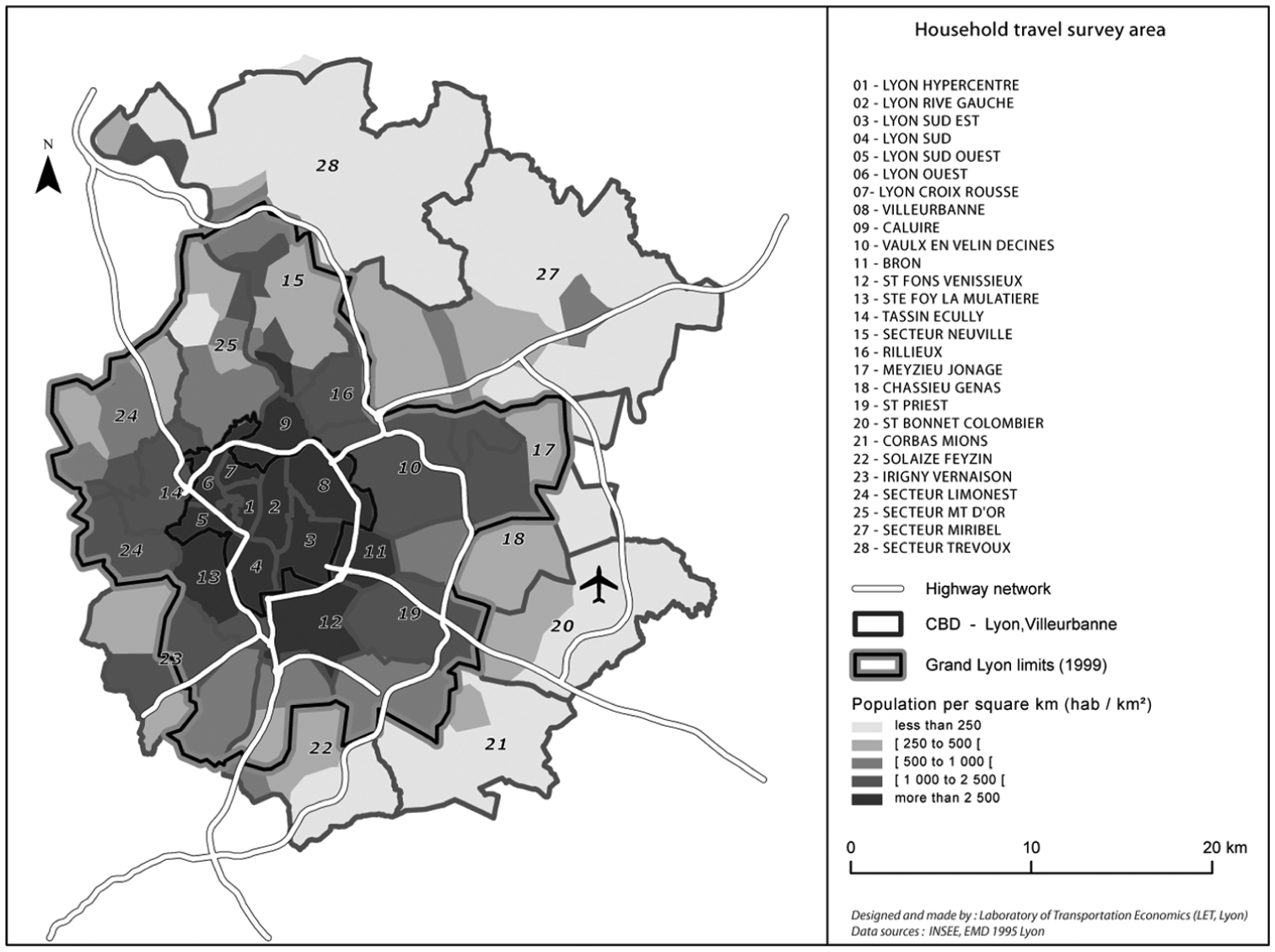
The study area: the Metropolitan Area of Lyon.

In addition to the availability of the data and the authors’ familiarity with its geography, this study area was chosen because of the announcement in the 2008 Protection Plan for the Lyon Metropolitan Area, that urban road pricing was a ‘possible’ scenario (Préfecture du Rhône, 2006). However, no perimeter for the toll zone or any toll charge has as yet been specified.

We have used data from the Household Survey, collected for the Lyon Metropolitan Area in 2006. This survey is performed every 10 years on a randomly selected sample and collects data on individuals and households including their socioeconomic characteristics, travel practices and residential locations. This data base pre-establishes annual net income brackets. Hypothesising that incomes are homogenously distributed within each income bracket makes it possible to use the average household income per consumption unit.⁷ This gives more precise information than the income decile, but does not solve the threshold effect problems linked to the breakdown of incomes into classes. Lerman and Yitzhaki (1989), Deltas (2003) and Wodon and Yitzhaki (2003) have shown that the use of grouped data induces a downward bias in the inequalities estimation. For example, in Lerman and Yitzaki (1989), grouping a sample of 64,000 observations into 30 groups of equal size caused a downwards bias in the Gini of 1.4% points, while grouping the data into five groups caused a bias of 8% points. Wodon and Yitzhaki (2003) give the following explanation: ‘This bias occurs because inequality measures can be decomposed into the sum of inter and intra-group inequality […]. Since grouping omits intra-group inequality, estimators of inequality based on grouped data reflect only inter-group inequality and therefore are biased downward’ (p. 153). Lastly, we withdrew non-responses to the question on income from the data base as otherwise setting them at zero would tend to lower the estimation of the Lorenz curve.⁸

The data used to calculate the accessibility indexes mostly concerned the cost of travel, estimated on the basis of the travel time between the 27 zones of the Lyon Metropolitan Area. To do this, all the sections of the roads of the city and their characteristics were incorporated into the MOSART simulation and modelling platform (Bonnafous et al., 2010), using the NAVTEQ⁹ road data for 2008. MOSART includes a multimodal transport model that estimates automobile traffic on each of the sections (for more details, see Mercier and Stoiber, 2010). Travel time is weighted by a VOT of 11.4€ corresponding to urban commuter travel, based on French administrative values (METATM, 2004). The cost of travel between zones i and j was weighted by the total number of jobs in zone j in 2003. The number of jobs in the Lyon Metropolitan Area between 2003 and 2006 was assumed to be constant. Since the actual 4% increase in the number of jobs (see INSEE, 2012) was almost constant for the entire Lyon Metropolitan Area, it did not affect the relative attractiveness of different zones.

Simulation of urban road pricing

We have simulated the implementation of boundary type urban road pricing around central Lyon and Villeurbanne (see CBD on Figure 1). This urban toll pricing has a double objective both to finance infrastructure and to reduce traffic flows and environmental impacts of traffic. The cordon area is based on two main ideas that lead us to think it will be the reasonable one. First, this central zone corresponds to the Central Business District where 44% of the population and 60% of the city’s jobs are located. It is quite usual to fix the cordon around the CBD (see London, for example). Second, the cordon limits are fixed to be also coherent with the natural limits given by the highway network (see Figure 1). All the drivers wishing to enter the central zone must pay the toll. The transit that bypasses the cordon area and traffic that stays inside the tolled central area does not pay the toll. We obtained the 5€ charge proposed in this study by updating the initial toll charge introduced in Oslo during peak hours.¹⁰ The toll charge of 0.11€ per km² which was applied in Oslo represented 0.05% of the median hourly wage in 2006. Here, a charge of 5€ is imposed on access to the centre of Lyon. Extending the surface area of the zone of 62 km², the charge amounts to 0.08€ per km², i.e. 0.05% of the median wage in 2004.¹¹

This price level is also coherent with the national price per kilometre bracket (1–3 euro/km) because a 5€ cordon price corresponds to a 2€/km price (the width of the Lyon Metropolitan Area is around 10 km). This tariff is consistent with those observed in urban tolled road infrastructures in France: see for example the existing Northern Toll Ring in Lyon (6.3 km) which is priced around 3€/km and the city tunnel (2.5 km) in Marseille (France) which is priced 1.12€/km. These rates are based on cost coverage of infrastructure projects rather than congestion relief.

As the level of toll depends on the objective of the scheme, a 5 euros rate points out the complexity of the French decision making, which is trying to mix two different objectives. Historically, the French toll system has an objective of financing infrastructure projects which induces a quite weak level of price (weak level of tariff to catch important traffic) (Raux and Souche, 2004). In the urban area, this major objective is now mixed with an objective of pricing to reduce traffic flows and environmental impacts of traffic. This double objective leads to a quite weak tariff of only 5 euros in Lyon, for example. This tariff is a little more than a tariff with only a financing objective (such as in Oslo with 15 NOK see Ramjerdi (1995) – e.g. 1.85 euros with 1 euro = 8.72296 NOK) as it integrates the objective to reduce flows. However, a rate of 5 euros is smaller than a congestion charging tariff as in London (£5 initially in London then an increase to £8 in July 2005 – around 7.5 and 12 euros see Raux et al., 2012). Obviously, congestion charging to reduce congestion with a high level of price seems to not be a priority in Lyon. We can formulate two main explanations. First, Lyon has less of a problem of congestion than London. Before the congestion charging introduction (by 2002), the all-day average travel speed was 14.3 km/h in central London (Leape, 2006). In central Lyon, the amount is between 15 km/h and 25 km/h according to time of day (see 2006 Household Survey). Second, the failure of a previous experiment in the 1990s (Raux and Souche, 2004) is always in mind in Lyon.

We have compared the situation before and after the introduction of road pricing. We have evaluated the impact of the toll on income concentration by measuring the before and after variation of the generalised cost of travel from i to j (dCg_ij). The latter is composed of a variation in the travel time from i to j (dt_ij) and a variation of the monetary cost of travel from i to j (dC_ij). Before the tolling, monetary cost refers to maintenance and fuel cost and after tolling it refers to fuel and maintenance cost and toll cost. Travel time cost is travel time multiplied by the VOT. With tolling implantation, travel cost is modified first with the introduction of toll cost payment, second by a change in travel time and thus in travel time cost.

Using v_m to denote the value of the household’s time, this variation can be written as follows:

d C g_{ij} = d C_{ij} + v_{m} d t_{ij}

(6)

In addition, the following hypotheses were made during simulation:

the variation of the generalised cost of travel from i to j corresponds to a variation of the average monthly net income of the household per consumption unit (dR_m). We can therefore write: dCg_ij = dR_m

the VOT in euros per minute, v_m, corresponds to the household’s net monthly income per consumption unit;¹²

the travel times between each of the zones correspond to the times taken by private car in the morning peak hours, calculated using the MOSART platform and taking account of congestion. We consider intra-zone travel time is null.

This study only considers the short-term impacts of the toll, consequently changes in the household residential or working factors are not taken into account.¹³

Consequently, dR_m is obtained with the following equation:

d R_{m} = d C_{ij} + v_{m} d t_{ij}

(7)

The inequality indicators (the Gini, Theil and Atkinson indices) were initially calculated on the basis of the household’s net monthly income per consumption unit. We then applied the variation of income dR_m resulting from the introduction of the toll charge to this income and recalculated the inequality indicators. This made it possible to compare the results for the different indicators before and after the toll.

The variation of accessibility is therefore written as follows:

d A_{i} = \sum_{j = 1}^{n} D_{j} dp + vd T_{ij}

(8)

where n is the number of zones, $D_{j}$ is the number of attractive forces in zone j, $d T_{ij}$ is the variation in travel time and $dp$ is the variation in the monetary cost of travel.

Results and analyses

We shall begin by presenting our results for the social inequality indicators, then those for spatial inequality (see data in Appendix 1).

Social inequality indicators

The results for the different social inequality indicators are contrasted at both the zonal level and the Lyon Metropolitan Area.

Change in social inequalities at the zonal level

From a general viewpoint, our findings regarding the Gini, Theil and Atkinson indices show that the effect of the toll differs in the different zones of the Lyon Metropolitan Area. In agreement with the literature, each index also gives different findings. The Theil and Atkinson indexes show the most marked differences and also the greatest differences between zones. They are also the only ones that show that introducing an urban toll can reduce inequalities for certain zones located outside the boundary, quite far from the toll zone. In other words, the toll is not a regressive measure for all zones.

When a toll zone is implemented, the Gini coefficient increases in all the zones, except peripheral zone 20 (Figure 2). In other words, the toll increases inequalities in all the zones of the Lyon Metropolitan Area. Thus, here, it is a regressive measure. The greatest increases in inequality in the Lyon Metropolitan Area are located in the most central zones (1 to 3), which are within the boundary, zones 10 and 12 in the inner ring and zone 17 in the outer ring. In these areas, the time savings do not offset the increase in travel cost.

Figure 2.

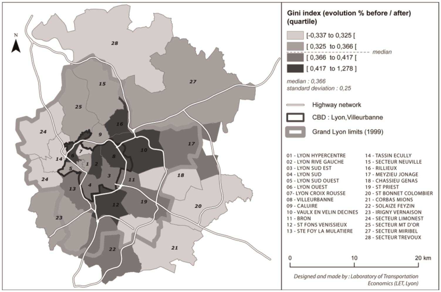
The Gini coefficient before/after the introduction of the urban toll.

Zone 20, which covers the east of Lyon, is an exception. It is a growth area which is marked out by the airport and is well served by road and rail. The attraction of the airport fuels local job demand and spurs the movement of employed persons into this zone (OPALE, 2007). The aim of introducing the toll was to charge traffic entering the centre of Lyon (from the outskirts to the centre in the morning). In this zone, the flows are from the centre to the periphery and from one peripheral area to another, thus not affected by the toll, although it does benefit from improved traffic flow in the periphery.

The results are more contrasted for the Theil index (see Figure 3). This fell in more than half the zones after the toll was introduced, which means the toll helped to reduce inequalities. Contrary to the commonly held view, this result means the toll appears to be a progressive measure. Theil’s index gave two other particularly interesting results: the inequalities fell in the tolled zone and increased in most of the zones outside but near to the toll boundary. The first result can be explained by speed gains in this zone and by non-payment of the toll by zone residents who do not cross the boundary. These two factors greatly reduce the negative impact of the toll. The second result is consistent with previous findings, in particular for Stockholm (Eliasson and Mattsson, 2006), which showed that the situation deteriorates particularly severely near the boundary.

Figure 3.

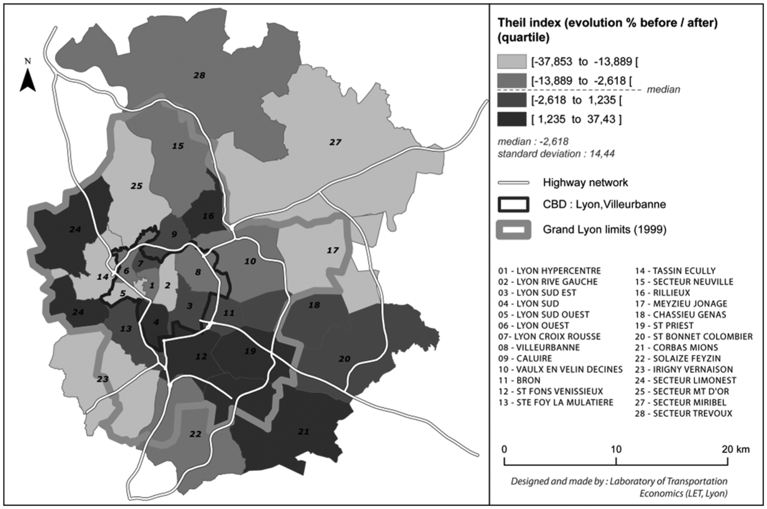
The Theil index before/after the introduction of the urban toll.

Lastly, central zones 4 and 5 are marked out by a negative value of the Theil index both before and after the toll was introduced. This means that in these cases a transfer occurs from the richest to the poorest. In other words, in these zones the toll does not interfere with the redistribution already in progress before its introduction. Zone 4 corresponds to the southern part of the 7th district of Lyon (Gerland). This zone is characterised by a large and dynamic area of employment specialised in the manufacture of pharmaceuticals (OPALE, 2009). We can therefore assume that this economic dynamism explains the redistributive capacity of this zone.

Like the Theil index, the results for the Atkinson index are contrasted, and rise or fall depending on the zone (Figure 4). In particular, the Atkinson indicator falls for the remoter peripheral zones 19 to 21 and 24 but rises for those of the centre and inner ring. In other words, the measure is progressive for certain remoter zones but regressive for those in the centre and inner ring.

Figure 4.

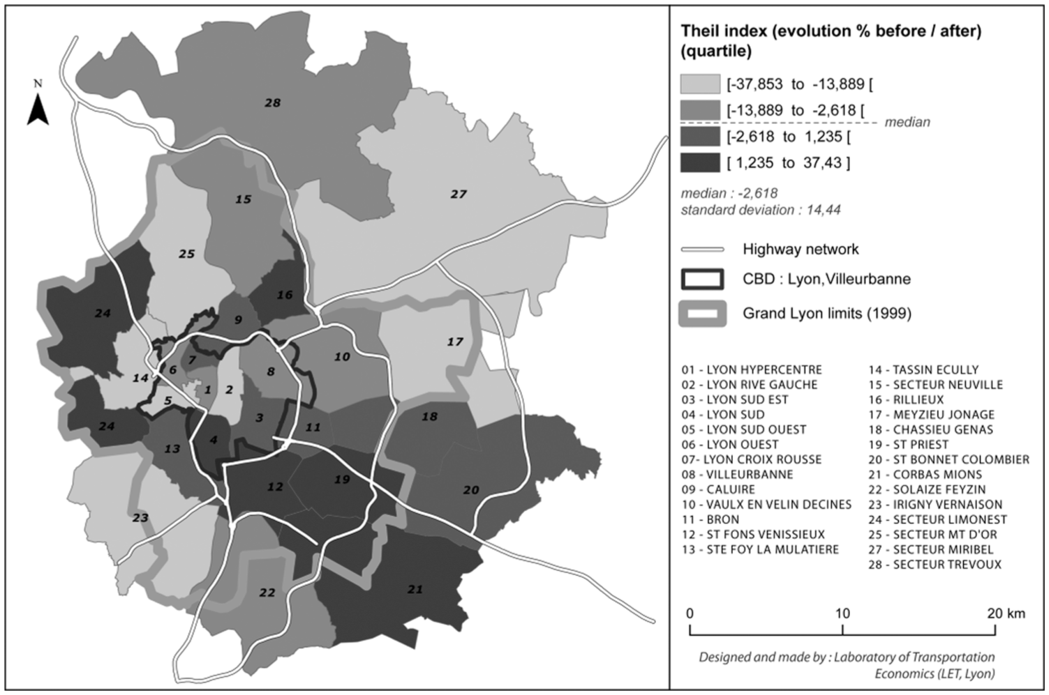
The Atkinson indicator before/after the introduction of the urban toll (ε = 1).

We test the sensitivity of Atkinson index measure to the inequality aversion parameter (see three epsilon values in Appendix 1). With ε = ½, results are in line with those for ε = 1 and ε = 2, except for zone 16 where variation becomes negative, showing a decrease in inequalities. This zone is characterised by a weaker average income. Consequently, as with ε = ½, inequality aversion is weaker, this result is quite coherent. However, our result shows that different epsilon values do not modify the sign of the Atkinson index variation. This confirms a decrease in inequalities for the furthest zones and an increase for most of the zone located near the cordon.

To sum up, if other indicators are considered in addition to the Gini coefficient, the urban toll does not appear to be a regressive measure for all zones. The Theil and Atkinson indicators show a decrease in inequalities for the furthest zones and an increase for most of the zones located near the toll boundary. In the first case, the payment of the toll is largely offset by time savings. In the second case, the time saving is not sufficient. Moreover, the Theil indicator is the only indicator that shows a reduction of inequalities for the central zones.

To test the robustness of our results, we have simulated three levels of price (3 euros, 5 euros, 7 euros; see Appendix 2). Results show that different levels of price have no influence on the level of the Gini indicator and that only a price of 5 euros induces change for Theil and Atkinson indicators. This finding justifies ex-post the use of 5 euros in the evaluation.

Changes in social inequalities at the scale of the Lyon Metropolitan Area

We now present aggregated changes in the Gini, Theil and Atkinson indicators values for the Lyon Metropolitan Area. Aggregated change is not the sum of changes mean for each zone. It means we use aggregated data without taking into account the zoning of the Lyon Metropolitan Area.¹⁴ Once again, the results are contrasted according to the indicator chosen, particularly in the case of the Theil and Atkinson indices.

At the scale of the Lyon Metropolitan Area, introducing the toll leads to an increase in the Gini indicator from 0.34 to 0.35, indicating that it is a regressive measure that increases social inequalities.

The results for the Theil indicator contrast strongly with the results for those of the Gini and Atkinson indicators, as its value becomes negative following the introduction of the toll. Its fall from 0.27 to −0.06 means that the introduction of the toll leads to a transfer of income from the richest to the poorest. This redistributive dimension of the toll was, moreover, already present at the zonal scale. This observation should nonetheless be moderated as the negative value is mainly caused by the result for zone 4, detailed previously.

The Atkinson index for the whole Lyon Metropolitan Area increases, as does the Gini coefficient, meaning that the measure is regressive. It is the indicator with the largest variation, increasing more than threefold, from 0.20 to 0.66. Nonetheless, analysis on the scale of the Lyon Metropolitan Area slightly reduced the increase as it eliminated the distinction between centre and inner ring where the indicator increased, and more remote zones where inequalities decreased.

Change in spatial inequalities

A toll charge of 5€ to enter the central zone is responsible for an accessibility reduction of 13% for all the persons residing in the Lyon Metropolitan Area (Figure 5).

Figure 5.

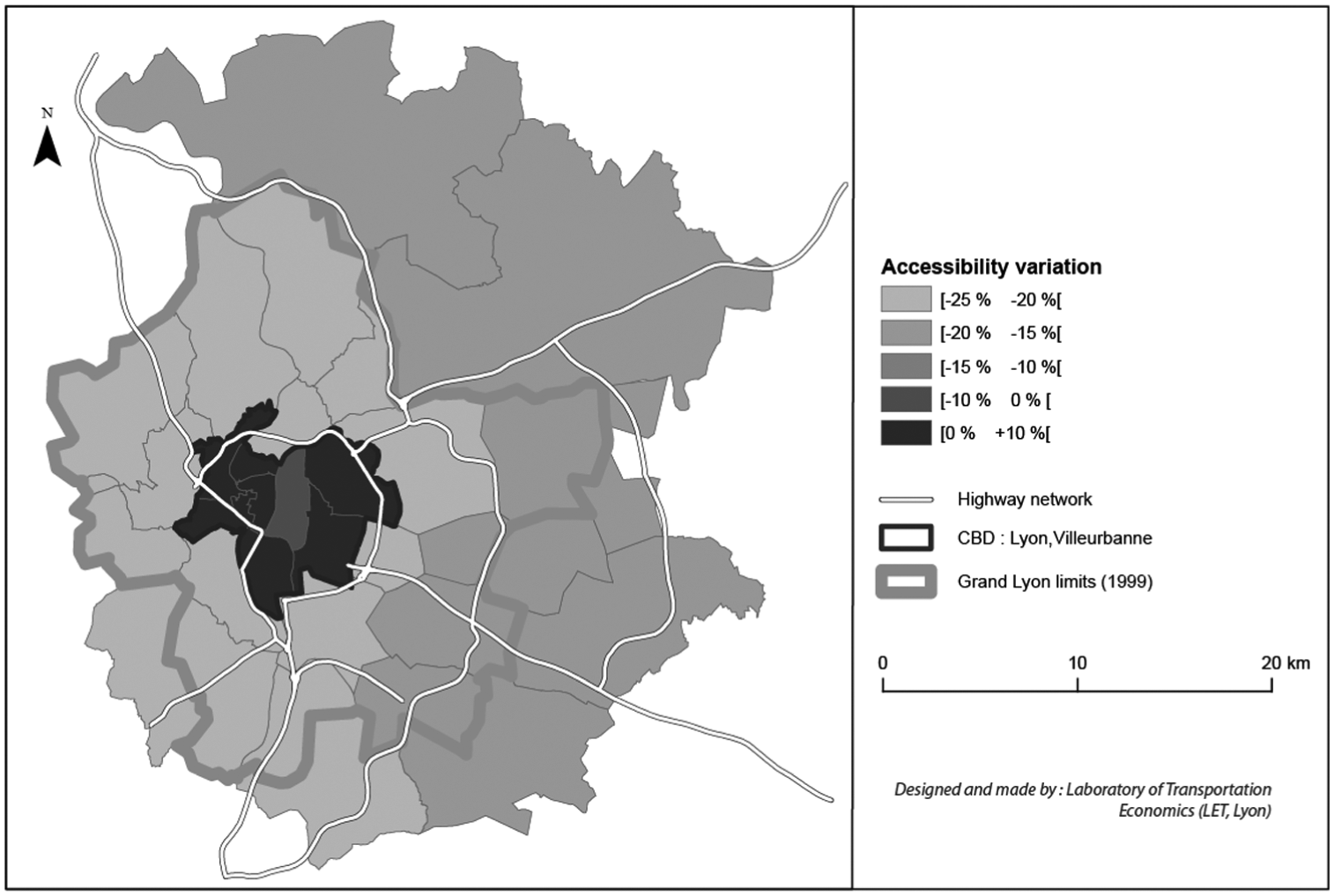
Variation of accessibility by zone following the introduction of a €5 toll charge.

This reduction does not affect all the zones to the same extent. Thus the level of accessibility remains stable and even increases for the working population residing inside the toll boundary. Zones 5 and 6 (southwest and west Lyon) benefit most from the introduction of the toll boundary. Indeed, the working population residing in the central zone does not have to pay the toll charge to travel to the locations of most of the jobs in the Lyon Metropolitan Area, i.e. the same central zone. However, although it is logical that the level of accessibility of this worker population does not decrease, how is it possible to explain that its accessibility ‘increases’?

Travel time has a strong impact on the level of accessibility. Introducing the toll zone results in a 4 percentage points reduction in total automobile traffic in the city centre, because of incoming traffic. The traffic is transferred to the three other modes. Modal share increase is respectively 1.3 for public transport, 1.9 for two-wheel modes and 0.8% for walking (for a 5 euros toll). However, as we will explain with a robustness test on price level, note that whatever the toll rate, modal shares and time savings are approximately constant. For a person whose job is located in the central zone, this reduction in automobile traffic generates an average time saving of 30 seconds to travel to jobs in the city centre and 40 seconds to travel to jobs outside it. These gains in time may appear small but when compared with the average trip time (about 8 minutes for trips within the central zone and 20 minutes for trips between all the zones of the Lyon Metropolitan Area), they represent a significant improvement in travel time.

The reduced accessibility of the zones in the first ring is a direct outcome of the increased monetary cost resulting from the toll charge. Since the toll boundary surrounds the zone with the highest number of jobs, workers living in the peripheral zones must pay 5€ to reach the jobs in the centre. This higher monetary cost is not – or only very partially – offset by the time saving resulting from less automobile traffic. The 4% reduction in automobile traffic over the whole Lyon Metropolitan Area results in an average timesaving of about two minutes to reach the centre from the different peripheral zones of the Lyon Metropolitan Area. With a VOT of 11.4€/h, it would be necessary to achieve a timesaving of 26 minutes or more to offset the cost of the toll.

The peripheral zones furthest from the centre appear to be subject to the lowest reductions in accessibility. The accessibility of these zones deteriorates by less than 20%. This relative reduction in accessibility is due to the time spent travelling from these zones to reach the centre and the fact that the toll represents a relatively small proportion of the total cost of travel.

We observe no significant correlation between the variation of accessibility and the initial level of accessibility. The zones with the greatest accessibility reduction (over 20%) have previously both low or high accessibility. But it is apparent that the cordon toll benefit to central zones that initially had among the best accessibility level to jobs. Thus, the toll zone would have a limited redistributive impact in the centre of the Lyon Metropolitan Area.

Figure 6 presents the variation of accessibility resulting from the toll introduction. Results show no significant correlation between the variation of accessibility and the working population in each zone. The zones for which the reduction of accessibility is highest were indiscriminately sparsely or densely populated. However, 75% of zones where an access decrease is observed are sparsely populated areas.

Figure 6.

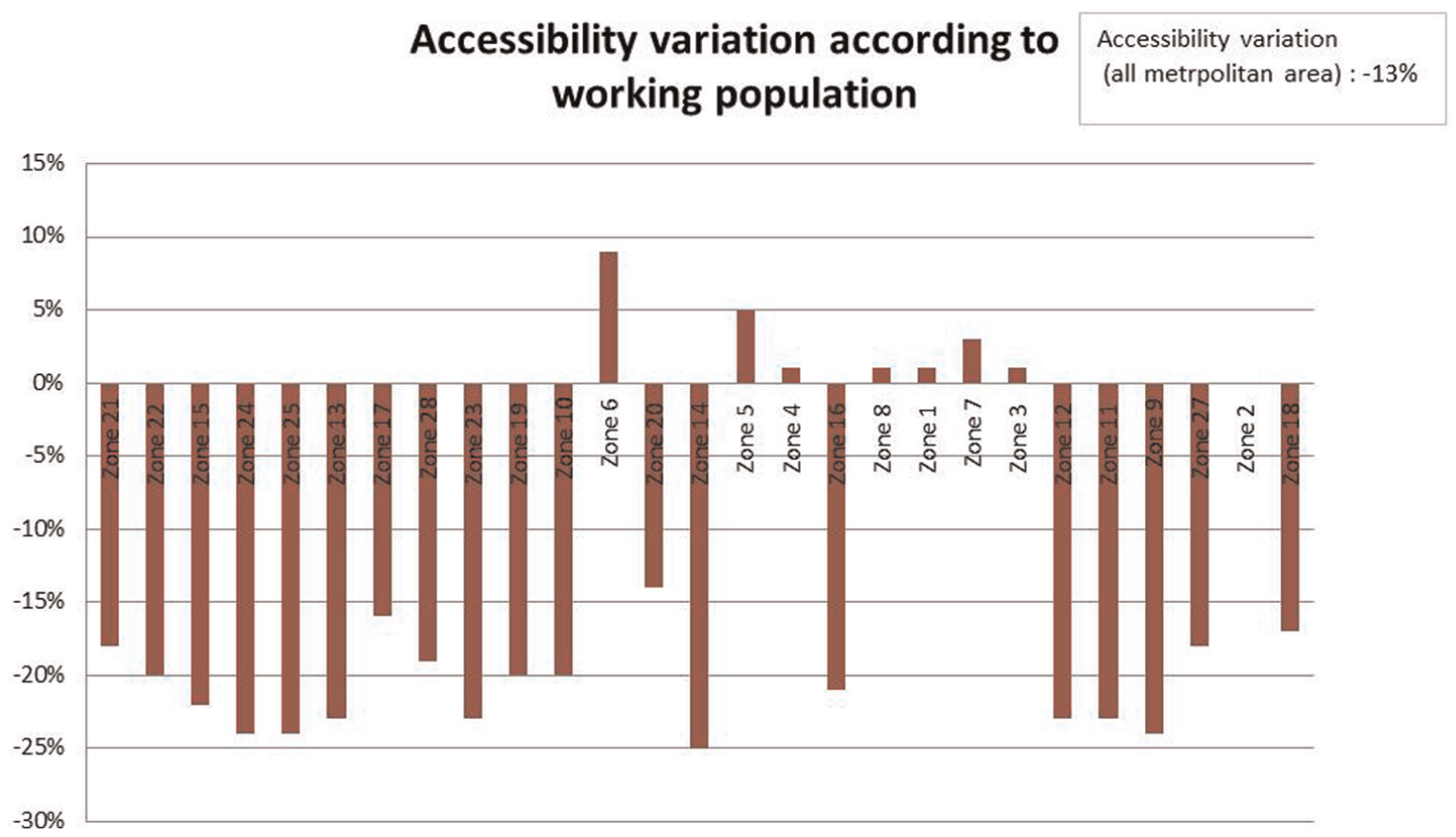
Variation of accessibility as a function of the working population by zone.

Comparing the measure of the variation of accessibility to the results of the inequality indicators can also provide interesting results. As we explain, introducing a cordon price does not particularly benefit the zones with the highest income inequalities. If we exclude zones 1, 2 and 3 because their level of accessibility remain constant, zones 11, 13 and 17 undergo an accessibility reduction ranging from 16% to 23%. By inhibiting access to centrally located jobs, the toll only exacerbates income inequalities between individuals with sufficient income to pay the charge (and thus working inside the city centre) and others. Lower income would shift to alternative modes or would look for work place(s) located outside the cordon area.

To test the robustness of our results, we have simulated three levels of price (3 euros, 5 euros, 7 euros; see Appendix 2). The trend observed with a 5€ tolling, compared with the base situation, is similar for a toll-fee at 3€ or 7€. Accessibility variations are smaller for 3€ than for 5€, and higher for 7€ than for 5€ even if variations are not linear with cordon toll pricing. This resulted mainly from negative exponential function used for mode choice. From a certain cordon price threshold, toll impacts on mode choice and therefore on travel time and accessibility is limited.

With only two minutes of travel time savings achieved from a 5 euro toll rate, our results seem to confirm the weak level of congestion in Lyon. Furthermore, as we show an increase of toll to 7 euros has a limited impact, in particular, on the accessibility variation, this result can be also interpreted as an argument against a congestion charging in Lyon meaning the congestion level is too small to implement congestion charging.

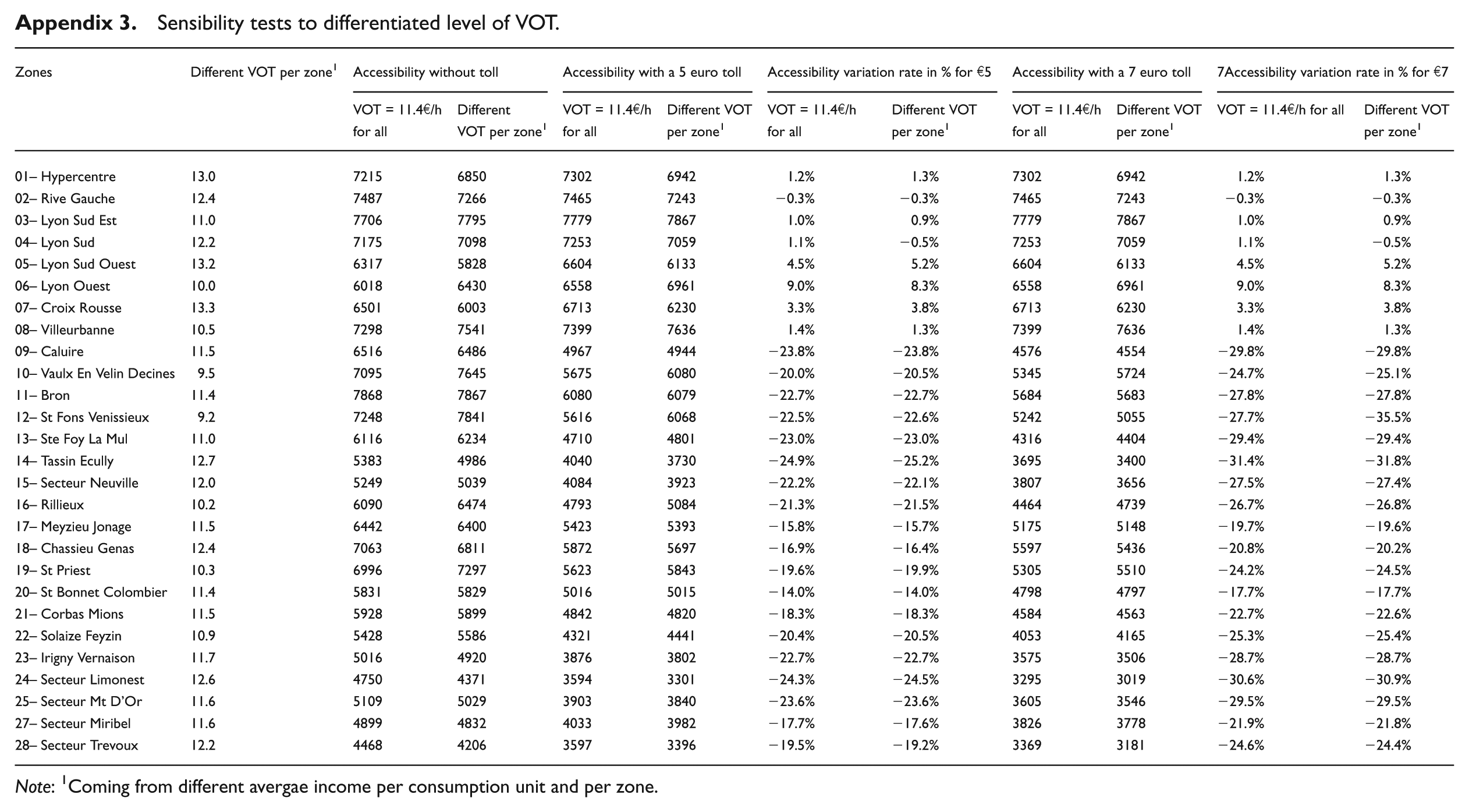
Furthermore, as spatial distribution of accessibility is expected to be affected by spatial distribution of income, we test the sensibility of this point. Sensibility tests introduce differentiated VOT determined according to level of income per consumption unit and per zone. The average income per consumption unit and per zone is computed from household’s income brackets coming from the Household Survey. Then VOT per zone is computed considering an income elasticity of 0.6 which is consistent with the literature (see Börjesson et al., 2012; Wardman and Shires, 2001) and with the reference value of 11.4€ per hour previously applied. Results show that spatial distribution of income does not significantly impact accessibility variations, except for a 7 euros rate for zone 12 (see Appendix 3). Three main explanations can explain such a weak effect. First, we have divided Lyon Metropolitan Area into quite large areas which can probably mask income disparities inside zones. At the same time, the level of income inequalities is probably lower in Lyon than in the rest of France (0.34 for Gini in Lyon Metropolitan Area against 0.38 for France; see Denis and Ruiz, 2009). Third, as previously explained, as travel time gains are very low, their monetary value therefore does not really impact accessibility results. Nevertheless, we can observe that accessibility variation tends to be in favour of ‘richest’ zones, with highest values of time, where accessibility decreases are relatively lower and accessibility increases higher than with a standard value-of-time. Furthermore, for a 7 euros rate, accessibility deterioration is higher for zone 12 (outside tolled area) when specific income dependent VOT is used. This result underlines toll negative impact for zone with a weak VOT.

Conclusion

This paper focuses on measurements of social and spatial inequalities and their variation following the introduction of an access charge to the central zones of the Lyon Metropolitan Area. We used three different indicators of social inequalities in association with a gravity-based measure of accessibility to provide information on spatial inequality. Analysis using before/after comparisons also allowed us to reduce the risk of the results being sensitive to the level of spatial division.

In conformity with the literature, we have found that different indicators of inequality produce contrasted and sometimes contradictory results, both at the zonal and metropolitan area levels. The number of zones (27), with a majority located outside the cordon, and the metropolitan surface of 62 km² can probably explain why we can achieve different results. However, pointing out different inequality indicators leads to different results is in line with Duro (2012). This result discourages the use of only one indicator for measuring inequalities and conducting zonal analyses.

Analysis by zone highlights an improvement of accessibility, in particular for the central zones. Moreover, it is interesting to observe that although the toll improves job accessibility from the centre of the city, this is particularly pronounced when the initial accessibility of the zone was poor. This observation does not hold, however, for the peripheral zones whose accessibility decreases because of the monetary cost of the toll. An average timesaving of two minutes to reach the city centre from the periphery during peak hours is not sufficient to offset this cost. Even if we had done a sensitivity analysis of the VOT value, which does not point out significant impact of spatial distribution of income on accessibility variations, in a future work it could be necessary to do a more disaggregated data and analysis in order to integrate others purposes and VOT per trip.

Our findings with regard to social inequalities are more surprising. On the one hand, the urban road pricing is not systematically a regressive measure as it can reduce inequalities to the same extent at the zonal scale as at that of the Lyon Metropolitan Area. However, this result cannot be obtained with the Gini indicator alone. On the other hand, it is the first ring, i.e. in our case the zone that is immediately outside the toll boundary, that is affected most negatively by the toll – a result which is confirmed by all three indicators. Lastly, only the Theil and Atkinson indicators showed that introducing a toll can reduce social inequalities for the most remote zones. In this case, the increased cost of travel is largely offset by time savings.

With regard to transport policy, our results underline the need for geographic compensatory measures for zones located within the first ring, for example by investing in a modal alternative with a good quality level. Furthermore, compensatory measures introduction induces a more general debate on the distributive approach used as reference in the transport field (see, for example, Martens, 2012; Raux and Souche, 2004; van Wee and Geurs, 2011). In the future, evaluating the revenue generated by urban tolls and their reinvestment in public transport infrastructure, especially in the inner ring, would allow us to adopt a multimodal approach and no longer consider inequalities with reference to a single mode. Furthermore, as we show theses three indicators can give contradictory results, in a future work it could be useful to test systematically all the inequality indicators.

Footnotes

Appendix

Appendix 3.

Sensibility tests to differentiated level of VOT.

Zones	Different VOT per zone¹	Accessibility without toll		Accessibility with a 5 euro toll		Accessibility variation rate in % for €5		Accessibility with a 7 euro toll		7Accessibility variation rate in % for €7
		VOT = 11.4€/h for all	Different VOT per zone¹	VOT = 11.4€/h for all	Different VOT per zone¹	VOT = 11.4€/h for all	Different VOT per zone¹	VOT = 11.4€/h for all	Different VOT per zone¹	VOT = 11.4€/h for all	Different VOT per zone¹
01– Hypercentre	13.0	7215	6850	7302	6942	1.2%	1.3%	7302	6942	1.2%	1.3%
02– Rive Gauche	12.4	7487	7266	7465	7243	−0.3%	−0.3%	7465	7243	−0.3%	−0.3%
03– Lyon Sud Est	11.0	7706	7795	7779	7867	1.0%	0.9%	7779	7867	1.0%	0.9%
04– Lyon Sud	12.2	7175	7098	7253	7059	1.1%	−0.5%	7253	7059	1.1%	−0.5%
05– Lyon Sud Ouest	13.2	6317	5828	6604	6133	4.5%	5.2%	6604	6133	4.5%	5.2%
06– Lyon Ouest	10.0	6018	6430	6558	6961	9.0%	8.3%	6558	6961	9.0%	8.3%
07– Croix Rousse	13.3	6501	6003	6713	6230	3.3%	3.8%	6713	6230	3.3%	3.8%
08– Villeurbanne	10.5	7298	7541	7399	7636	1.4%	1.3%	7399	7636	1.4%	1.3%
09– Caluire	11.5	6516	6486	4967	4944	−23.8%	−23.8%	4576	4554	−29.8%	−29.8%
10– Vaulx En Velin Decines	9.5	7095	7645	5675	6080	−20.0%	−20.5%	5345	5724	−24.7%	−25.1%
11– Bron	11.4	7868	7867	6080	6079	−22.7%	−22.7%	5684	5683	−27.8%	−27.8%
12– St Fons Venissieux	9.2	7248	7841	5616	6068	−22.5%	−22.6%	5242	5055	−27.7%	−35.5%
13– Ste Foy La Mul	11.0	6116	6234	4710	4801	−23.0%	−23.0%	4316	4404	−29.4%	−29.4%
14– Tassin Ecully	12.7	5383	4986	4040	3730	−24.9%	−25.2%	3695	3400	−31.4%	−31.8%
15– Secteur Neuville	12.0	5249	5039	4084	3923	−22.2%	−22.1%	3807	3656	−27.5%	−27.4%
16– Rillieux	10.2	6090	6474	4793	5084	−21.3%	−21.5%	4464	4739	−26.7%	−26.8%
17– Meyzieu Jonage	11.5	6442	6400	5423	5393	−15.8%	−15.7%	5175	5148	−19.7%	−19.6%
18– Chassieu Genas	12.4	7063	6811	5872	5697	−16.9%	−16.4%	5597	5436	−20.8%	−20.2%
19– St Priest	10.3	6996	7297	5623	5843	−19.6%	−19.9%	5305	5510	−24.2%	−24.5%
20– St Bonnet Colombier	11.4	5831	5829	5016	5015	−14.0%	−14.0%	4798	4797	−17.7%	−17.7%
21– Corbas Mions	11.5	5928	5899	4842	4820	−18.3%	−18.3%	4584	4563	−22.7%	−22.6%
22– Solaize Feyzin	10.9	5428	5586	4321	4441	−20.4%	−20.5%	4053	4165	−25.3%	−25.4%
23– Irigny Vernaison	11.7	5016	4920	3876	3802	−22.7%	−22.7%	3575	3506	−28.7%	−28.7%
24– Secteur Limonest	12.6	4750	4371	3594	3301	−24.3%	−24.5%	3295	3019	−30.6%	−30.9%
25– Secteur Mt D’Or	11.6	5109	5029	3903	3840	−23.6%	−23.6%	3605	3546	−29.5%	−29.5%
27– Secteur Miribel	11.6	4899	4832	4033	3982	−17.7%	−17.6%	3826	3778	−21.9%	−21.8%
28– Secteur Trevoux	12.2	4468	4206	3597	3396	−19.5%	−19.2%	3369	3181	−24.6%	−24.4%

Note: ¹Coming from different avergae income per consumption unit and per zone.

Acknowledgements

The authors would like to thank the three reviewers of Urban Studies for their constructive comments.

Funding

This research received no specific grant from any funding agency in the public, commercial, or not-for-profit sectors.

Notes

References

Almas

Cappelen

Lind

. (2011) Measuring unfair (in)equality. Journal of Public Economics95: 488–499.

Amiel

Cowel

(1992) Measurement of income inequality. Experiments test by questionnaire. Journal of Public Economics47: 3–26.

Atkinson

Bourguignon

(eds) (2007) Handbook of Income Distribution. Handbook in Economics 16, Elsevier, North-Holland, 918 pp.

Atkinson

(1970) On the measurement of inequality. Journal of Economic Theory55: 244–263.

Bhat

Handy

Kockelman

. (2000) Development of an urban accessibility index: Literature review. Research project 7–4938–1. Available at: www.utexas.edu/research/ctr/pdf_reports/4938_4.pdf, 92 pp.

Bonnafous

Crozet

Mercier

. (2010) MOSART et le projet PLAINSUDD: Une plate-forme de modélisation et de simulation de l’accessibilité pour l’aide à la décision et l’aménagement du territoire. In: Antoni

J-P

(ed.) Modéliser la ville. Predit: Economica, pp. 186–210.

Bonsall

Kelly

(2005) Road user charging and social exclusion: The impact of congestion charges on at-risk groups. Transport Policy12: 406–418.

Börjesson

Fosgerau

Algers

(2012) On the income elasticity of the value of travel time. Transportation Research Part A46: 368–377.

Chakravarty

(1996) A measurement of spatial disparity: The case of income inequality. Urban Studies33(9): 1671–1996.

10.

Chakravarty

(1999) Measuring inequality: The axiomatic approach. In: Silber

(ed.) Handbook of Income Inequality Measurement. Dordrecht: Kluwer Academic Publishers, pp. 163–186.

11.

Church

Frost

Sullivan

(2000) Transport and social exclusion in London. Transport Policy7: 195–205.

12.

Condeço-Melhorado

Gutierrez

Garcia-Palomares

(2011) Spatial impacts of road pricing: Accessibility, regional spillovers and territorial cohesion. Transportation Research Part A45: 185–203.

13.

Cowel

(2000) Measurement of inequality. In: Atkinson

Bourguignon

(eds) Handbook of Income Distribution, 1, Collect. Handbooks in Economics 16, Amsterdam: Elsevier, pp. 84–166.

14.

Cowell

Flachaire

(2007) Income distribution and inequality measurement: The problem of extreme values. Journal of Econometrics141: 1044–1072.

15.

Dagum

(1980) Inequality measures between income distributions with applications. Econometrica48(7): 1791–1803.

16.

Deltas

(2003) The small sample bias of the Gini coefficient: Results and implications for empirical research. Review of Economics and Statistics85(1): 226–234.

17.

Denis

Ruiz

(2009) Mesurer les inégalités. Cahiers Français351: La Documentation Française, pp. 22–28.

18.

Dial

(1999) Minimal-revenue congestion pricing part I: A fast algorithm for the single-origin case. Transportation Research Part B33: 189–202.

19.

Duranton

Overman

(2005) Testing for localization using micro-geographic data. The Review of Economic Studies72(4): 1077–1106.

20.

Duro

(2012) On the automatic application of inequality indexes in the analysis of the international distribution of environmental indicators. Ecological Economics76: 1–7.

21.

Eliasson

(2009) Lessons from the Stockholm congestion charging trial. Transport Policy15(6): 395–404.

22.

Eliasson

Mattsson

L-G

(2006) Equity effects of congestion pricing. Quantitative methodology and a case study for Stockholm. Transportation Research Part A40: 602–620.

23.

Evans

(1992) Road congestion pricing: When is it a good policy?Journal of Transport Economics and Policy26: 213–244.

24.

Fotheringham

O’Kelly

(1989) Spatial Interaction Model: Formulations and Applications. Dortrecht, Boston, London: Kluwer Academic Publishers, 244 pp.

25.

Geurs

van Wee

(2004) Accessibility evaluation of land-use and transport strategies: Review and research directions. Journal of Transport Geography12: 127–140.

26.

Gini

(1921) Measurement of inequality of incomes, Economic Journal31: 124–126.

27.

Giuliano

(1992) An assessment of the political acceptability of congestion pricing. Transportation19(4): 335–358.

28.

Glazer

(1981) Congestion tolls and consumer welfare. Public Finance36: 77–83.

29.

Grengs

(2010) Job accessibility and the modal mismatch in Detroit. Journal of Transport Geography18: 42–54.

30.

Guttman

(1975) Avoiding specification errors in estimating the value of time. Transportation4: 19–42.

31.

Handy

(1992) Regional versus local accessibility: Neo-traditional development and its implications for non-work travel. Built Environment18: 253–267.

32.

Handy

(1993) A cycle of dependence: Automobiles, accessibility, and the evolution of the transportation and retail hierarchies. Berkeley Planning Journal8: 21–43.

33.

Handy

Niemeier

(1997) Measuring accessibility: An exploration of issues and alternatives. Environment and Planning A29: 1175–1194.

34.

Hansen

(1959) How accessibility shapes land use. Journal of the American Institute of Planners25: 73–76.

35.

Holl

(2007) Twenty years of accessibility improvements. The case of the Spanish motorway building program. Journal of Transport Geography15: 86–297.

36.

Hou

S-M

(2011) Transport infrastructure development and changing spatial accessibility in the Greater Pearl River Delta, China, 1990–2020. Journal of Transport Geography19: 1350–1360.

37.

Iacono

Krizek

El-Geneidy

(2010) Measuring non-motorised accessibility: Issues, alternatives, and execution. Journal of Transport Geography18: 133–140.

38.

Institut National de la Statistique et des Etudes Economiques (INSEE) (2012) Estimation d’emploi par zone d’emploi et secteur d’activité de 1998 à 2009. Available at: http://www.insee.fr/fr/themes/detail.asp?reg_id=99&ref_id=emploi-zone-2008.

39.

Jenelius

Mattsson

L-G

Levinson

(2011) Traveler delay costs and value of time with trip chains, flexible activity scheduling and information. Transportation Research Part B45: 789–807.

40.

Jones

Lucas

(2012) The social consequences of transport decision making: Clarifying concepts, synthesizing knowledge and assessing implications. Journal of Transport Geography21: 4–16.

41.

Karlström

Franklin

(2009) Behavioral adjustments and equity effects of congestion pricing: Analysis of morning commuters during Stockholm trial. Transportation Research Part A43: 283–296.

42.

Koenig

(1980) Indicators of urban accessibility: Theory and application. Transportation9: 145–172.

43.

Kwan M-P (1998) Space–time and integral measures of individual accessibility: A comparative analysis using a pointbased framework. Geographical Analysis30(3): 191–216.

44.

Kwan

Weber

(2008) Scale and accessibility: Implications for the analysis of land use-travel interaction. Applied Geography28: 110–123.

45.

Leape

(2006) The London congestion charge. Journal of Economic Perspectives20(4): 157–176.

46.

Lerman

Yitzhaki

(1989) Improving the accuracy of estimates of Gini coefficient. Journal of Econometrics42: 43–47.

47.

Limanond

Niemeier

(2003) Accessibility and mode-destination choice decisions: Exploring travel in three neighborhoods in Puget Sound, WA. Environment and Planning B30: 219–228.

48.

Martens

(2012) Justice in transport as justice in accessibility: Applying Walzer’s ‘Spheres of Justice’ to transport sector. Transportation39(6): 1–19.

49.

Mayeres

Proost

(2001) Marginal tax reform, externalities and income distribution. Journal of Public Economics79: 343–363.

50.

Mercier

Stoiber

(2010) Improving accessibility measurement combining transport modelling and GIS analysis: Two examples from France and Germany. In: Viegas

Macario

(eds) Selected Proceedings of the 12th WCTR. Lisbon.

51.

Ministère de l’Equipement, des Transports, de l’Aménagement du territoire, du Tourisme et de la Mer (METATM) (2004) Instruction cadre relative aux méthodes d’évaluation économique des grands projets d’infrastructures de transport. METATM. Available at: dtrf.setra.fr/notice.html?id=Dtrf-0003601, 31 pp. + annex.

52.

Morris

Dumble

Wigan

(1978) Accessibility indicators for transport planning. Transportation Research A13: 91–109.

53.

Mun

S-E

Ahn

K-J

(2008) Road pricing in a serial network. Journal of Transport Economics and Policy42(3): 367–395.

54.

Observatoire Partenarial Lyonnais en Economie (OPALE) (2007) CCI Est lyonnais. OPALE. Available at: www.opale-lyon.com, 13 pp.

55.

Observatoire Partenarial Lyonnais en Economie (OPALE) (2009) Les territoires de l’économie lyonnaise – Lyon 7ème. OPALE. Available at: www.opale-lyon.com, 13 pp.

56.

Ortuzar

J-D

Willumsen

(2002) Modelling Transport. 3rd Edition.Chichester: Wiley and Sons, 499 pp.

57.

Préfecture du Rhône (2006) Plan de Protection de l’Atmosphère de l’agglomération lyonnaise. Available at: http://ppalyon.nerim.net/PPA_2005_2010.pdf, 164 pp.

58.

Ramjerdi

(1995) Road Pricing and Toll Financing with Examples from Oslo and Stockholm. Washington, DC: KTH and TOI, 147 pp.

59.

Ramjerdi

(2006) Equity measures and their performance in transportation. Journal of Transportation Record Board1983: 67–74.

60.

Raux

Souche

(2004) The acceptability of urban road pricing: A theoretical analysis applied to experience in Lyon. Journal of Transport Economics and Policy38(2): 191–216.

61.

Raux

Mercier

Ovtracht

(2008) Evaluation économique des politiques de transport et indicateurs d’accessibilité spatiale: l’apport des SIG. Cybergeo: European Journal of Geography, Systèmes, Modélisation, Géostatistiques DOI: 10.4000/cybergeo.21333, document 435. Available at: http://cybergeo.revues.org/21333.

62.

Raux

Souche

Pons

(2012) The efficiency of congestion charging: Some lessons from cost-benefit analyses. Research in Transportation Economics36: 85–92.

63.

Reggiani

Bucci

Russo

. (2011a) Regional labour markets and job accessibility in city network systems in Germany. Journal of Transport Geography9(4): 528–536.

64.

Reggiani

Bucci

Russo

(2011b) Accessibility and impedance forms: Empirical applications to the German commuting network. International Regional Science Review34(2): 230–252.

65.

Richardson

(1974) A note on the distribution effects of road pricing. Journal of Economics and Policy8(1): 82–85.

66.

Rietveld

Verhoef

(1998) Social feasibility of policies to reduce externalities in transport. In: Button

Verhoef

(eds) Road Pricing, Traffic Congestion and the Environment. Cheltenham: E Elgar, Chapter13.

67.

Rotaris

Danielis

Marcucci

. (2010) The urban road pricing scheme to curb pollution in Milan, Italy: Description, impacts and preliminary cost–benefit analysis assessment. Transportation Research Part A44(5): 359–375.

68.

Rouwendal

Verhoef

(2006) Basic economic principles of road pricing: From theory to applications. Transport Policy13: 106–114.

69.

Santos

Rojey

(2004) Distributional impacts of road pricing: The truth behind the myth. Transportation31(1): 21–42.

70.

Shorrocks

(1980) The class of additively decomposable inequality measures. Econometrica48: 613–625.

71.

Song

(1996) Some tests of alternative accessibility measures: A population density approach. Land Economics72(4): 474–482

72.

Spence

Linneker

(1994) Evolution of the motorway network and changing levels of accessibility in Great Britain. Journal of Transport Geography2(4): 247–264.

73.

Sumalee

May

Shepherd

(2005) Comparison of judgmental and optimal road pricing cordons. Transport Policy12: 384–390.

74.

Theil

(1967) Economics and Information Theory. Amsterdam: North Holland Publishing Company.

75.

Theriault

Voisin

Des Rosiers

(2008) L’accessibilité aux services urbains: Modélisation des différences socio-spatiales et mesure des impacts sur les valeurs résidentielles. In: Theriault

Des Rosiers

(eds) Information géographique et dynamiques urbaines, 2. London: Hermes Sciences Publishing, pp. 119–151.

76.

Tillema

Verhoef

Wee

. (2011) Evaluating the effects of urban congestion pricing: Geographical accessibility versus social surplus. Transportation Planning and Technology34(7): 669–689.

77.

Van Wee

Geurs

(2011) Discussing equity and social exclusion in accessibility evaluations. European Journal of Transport and Infrastructure Research11(4): 350–367.

78.

Wardman

Shires

(2001) Intertemporal variations in the value of time. Working Paper, 566. Available at: eprints.whiterose.ac.uk/2060/1/ITS35_WP566_uploadable.pdf, 28 pp.

79.

Willigers

Floor

Van Wee

(2007) Accessibility indicators for location choices of offices: An application to the intraregional distributive effects of high-speed rail in the Netherlands. Environment and Planning A39: 2086–2098.

80.

Wodon

Yitzhaki

(2003) The effect of using grouped data on the estimation of the Gini income elasticity. Economics Letters78:153–159.