Differences in housing price dynamics across cities: A comparison of different panel model specifications

Abstract

This study compares a conventionally used panel data model – that does not allow for regional variations in housing price dynamics – with panel models that let the dynamics differ across regions. We concentrate on examining the momentum dynamics and the reversion speed towards the fundamental price level. Based on data over 1988–2012, the results indicate that the regional differences are generally quite small in the Finnish market. Nevertheless, in several cities the dynamics differ significantly from those indicated by the baseline model that does not allow for regional variation. In addition, the long-term coefficient on income considerably varies across regions, the coefficient being greater in the more supply-constrained cities. The results indicate that the use of panel models that assume similar housing price dynamics across regions can lead to flawed conclusions being drawn.

Keywords

bubble dynamics housing price momentum panel data

Introduction

The understanding of housing price dynamics is of importance to a great number of agents: to portfolio investors, banks, real estate brokers and construction companies as well as to policy makers and households. Unfortunately, the data that are used to study housing price dynamics empirically are generally problematic. One complication is the relatively low frequency of data on housing prices and on the fundamentals that significantly affect housing prices. Reliable housing price information is typically available only at the quarterly or, at best, monthly frequency. Moreover, data on some of the economic fundamentals that are expected to drive housing prices are only available at an annual frequency in many markets.

Given the low frequency of data and the relatively short sample periods available, the econometric analyses examining housing price dynamics often exhibit small-sample complications. Therefore, a number of studies (e.g. Bramley and Leishman, 2005; Capozza et al., 2004; Harter-Dreiman, 2004; Lamont and Stein, 1999) investigate housing price dynamics using panel data models. By combining cross-sectional data, for instance multiple cities or countries, with the time series property of data, panel data analysis increases the number of observations and thereby the degrees of freedom in econometric modelling.

A potential complication with many of the panel data analyses is the use of ‘conventional’ fixed-effects models. ‘Conventional’ refers here to the models that assume housing price dynamics to be the same in every region included in the analysis. The parameters reported in the previous panel data analyses investigating housing price dynamics are generally average values across all the regions included in the data. However, there are reasons to believe that the housing price elasticities with respect to fundamentals substantially vary across distinct regional housing markets (Capozza et al., 2004; Davis and Heathcote, 2007). Similarly, the magnitude of autocorrelation in housing price movements, i.e. housing price ‘momentum’, as well as the speed of adjustment towards the long-run fundamental price level may notably differ between housing markets (Capozza et al., 2004; Glaeser et al., 2008). Therefore, the use of conventional panel data models may yield misleading results regarding regional housing price dynamics. This may lead to suboptimal policy and investment decisions being made.

This study aims to examine empirically the magnitude of regional differences in housing price dynamics using annual data for 14 Finnish cities for the period 1988–2012. Given the implications of urban economics theory and extant empirical literature, we hypothesise that there are significant regional differences in the momentum effect of housing prices (‘bubble builder’), in the speed of adjustment of housing prices towards their long-run fundamental level (‘bubble burster’), and in the long-term elasticity of housing prices with respect to income. The results of the baseline model, i.e. the conventionally used fixed-effects panel model, are compared with those of less restrictive models where the dynamics are allowed to vary across cities. The analysis can also be seen as a test for the validity of conventionally used panel models to analyse regional housing price dynamics.

The study contributes to the literature by being the first panel analysis that allows for regional differences in both the long- and short-term housing price dynamics and that formally tests for the significance of regional differences in the dynamics – we show how this can be done and provide a case study for the Finnish market. Moreover, unlike many of the previous related studies, we apply a dynamic panel estimator that excludes the endogeneity bias caused by the inclusion of lagged dependent variable as an explanatory variable. This also is the first rigorous application of dynamic panel techniques using Finnish housing market data. So far, most studies on housing price dynamics using panel data concentrate on the US market. Regarding the future research themes suggested by Bramley and Leishman (2005), the contribution of this article lies most prominently in modelling more explicitly the regional variations in housing price response behaviour.

While we find substantial regional differences in the long-term dynamics (income elasticity), the panel estimations indicate that the regional variation in the short-run housing price dynamics across Finnish cities is relatively small. Nevertheless, in many cities even the short-term dynamics differ significantly from those indicated by the baseline model that does not allow for regional variation. This shows that the conventionally used models yield misleading estimates at least for some regional housing markets, supporting our main hypothesis according to which the models not allowing for regional differences may lead to worse decisions and conclusions than models that cater more rigorously for regional variation.

In addition, the results provide evidence of cointegration between housing prices and per capita income. While cointegration is detected between housing prices and income in all the 14 cities, the long-run income elasticity considerably varies across cities. In general, the elasticity is the greater, the larger and more supply constrained is the city.

Considerations on regional differences in housing price dynamics

Land leverage and regional housing price dynamics

The value of land is expected to be a central factor causing regional differences in housing price elasticities with respect to economic fundamentals. Since desirable land is largely non-reproducible, changes in the demand for housing are likely to have substantial influences on the price of the land component of housing. By contrast, housing demand changes are expected to have a notably smaller impact on the real value of structures. A likely outcome is that the residential land value volatility is considerably greater than that of housing structures. Empirical evidence supporting this suggestion is provided in Davis and Heathcote (2007) and Gyourko and Saiz (2006).

The different dynamics of land prices and construction costs indicate that housing price dynamics should be quite different in regions where the value of housing is largely accounted for by the value of land, i.e. where the ‘land leverage’ is high, compared with regions where land leverage is relatively low (Bostic et al., 2007; Bourassa et al., 2011; Davis and Heathcote, 2007).¹ Obviously, land leverage is closely related to supply constraints on land. Other things equal, tighter supply constraints and lower supply elasticity lead to greater land leverage.

Conventionally, panel data analyses on housing price dynamics have been based on models that assume the parameters on fundamentals to be the same regardless of the region (e.g. Jud and Winkler, 2002; Lamont and Stein, 1999). Given that land leverage appears to substantially vary between regions (Bostic et al., 2007; Davis and Heathcote, 2007), the assumption of similar parameters across regions may be flawed. In the Finnish case, for instance, the effect of income growth on housing price level is expected to be greater in Helsinki, where land leverage is high, than in the considerably smaller city of Rovaniemi, where the value of land is considerably lower.

In the conventionally used panel models, housing appreciation rates are allowed to vary across areas not only because of regional differences in the evolution of market fundamentals but also because of location-specific fixed-effects. These fixed-effects control for time-invariant unobserved determinants of house prices and represent the residuals of housing price appreciation attributable to location (Jud and Winkler, 2002). The important question is: what is the factor that the fixed-effects try to take account of? In other words, why would prices in one location rise more than in another location even if the development of market fundamentals was exactly the same in both markets? Obviously, the reason for the different appreciation rates is the market specific elasticities of housing prices with respect to fundamentals. The conventionally used panel models cannot cater properly for this regional heterogeneity, and may thereby lead to biased conclusions concerning regional housing price dynamics.

Housing price momentum and reversion towards the fundamental price level

Housing prices have been shown to exhibit notable short-run persistence and long-run mean reversion (e.g. Beracha and Skiba, 2011; Capozza et al., 2004; Case and Shiller, 1989, 1990; Roed Larsen and Weum, 2008). Abraham and Hendershott (1996) call the short-term positive autocorrelation, i.e. the short-term momentum, a ‘bubble builder’ because of its tendency to often drive housing prices further away from their fundamental level. The reverting tendency of housing prices towards their long-run fundamental level, in turn, is often referred to as a ‘bubble burster’. The magnitude of momentum and strength of reversion towards the fundamental level are of great importance regarding housing price dynamics, not least because of their predictability implications and their influence on the occurrence and magnitude of housing price cycles and bubbles. Importantly, the momentum and reversion dynamics may significantly vary across regions.

In the housing market, backward-looking expectations are likely to strengthen the momentum effect. For instance, Capozza et al. (2004) and Dusansky and Koç (2007) present evidence of backward-looking expectations in the housing market. Various informational factors can influence the significance of such feedback effects in a given market.

Clapp et al. (1995) suggest that higher population density should foster more, better and more prompt information concerning the housing market, since information production is subject to positive scale economies. Moreover, in markets with a greater number of transactions, information costs are lower and, therefore, prices should respond more rapidly to changing fundamentals (Capozza et al., 2004). In line with these arguments, empirical evidence suggests that people show stronger behavioural biases driven by psychological constraints when the asset is harder to value (Hirshleifer et al., 2013; Kumar, 2009). Generally, housing is easier to value in an area with a greater number of transactions and thereby greater information flows.

Overall, these informational factors suggest that in larger and more densely populated metropolitan areas with more liquid housing market, behavioural biases such as backward-looking expectations should be less significant and housing demand should more rapidly adjust to shocks. Therefore, in these kinds of regions the adjustment towards fundamental price level should be more rapid and the momentum effect is expected to be weaker.

However, there can also be other reasons than the informational factors that cause regional variation in housing price momentum and reversion. Capozza et al. (2004) hypothesise that higher real construction costs are correlated with slower reversion and greater serial correlation. The results of Hwang and Quigley (2006) emphasise the importance of local regulation (i.e. administrational supply restrictions) on housing market dynamics. Furthermore, in less densely populated areas supply may be able to adjust more rapidly than in areas with greater density and scarcity of land (Glaeser et al., 2008).

Since the informational and (other) structural factors may have opposite effects on housing price persistence and reversion dynamics at the market level, it is essentially an empirical question to study the variation of price dynamics across regional housing markets. Unsurprisingly, some previous studies report notable regional differences in housing price dynamics (e.g. Bramley and Leishman, 2005; Capozza et al., 2004; Holly et al., 2010; Hwang and Quigley, 2006; Malpezzi, 1999; Wilhelmsson, 2008). On the other hand, Englund and Ioannides (1997) find the autocorrelation structures to be strikingly similar across countries.

The panel data analyses studying housing price dynamics typically have not considered potential regional differences. There are some exceptions, however. Holly et al. (2010) allow the short-term dynamics to vary across US regions. In Malpezzi (1999), the adjustment speed towards fundamental price level varies across US areas, while Capozza et al. (2004) let both the adjustment speed and momentum differ across US metro areas, and Abraham and Hendershott (1996) estimate separate models for coastal cities and inland cities in the US. Lamont and Stein (1999) allow for regional variation in the coefficient on income change, but they neither present the range of point estimates nor test formally for the significance of the regional variation.

Bramley and Leishman (2005) and Wilhelmsson (2008) provide two of the rare studies not using US data. Wilhelmsson (2008) documents significant regional differences in the speed of equilibrium-adjustment in Sweden, faster adjustment occurring in regions with a low population density. Bramley and Leishman (2005), in turn, divide their UK panel data set into three broad area types to allow for regional variation. They find that housing market dynamics differ between markets that are characterised by low demand and those under high-demand pressure. Despite some recent research in the topic, the statement of Bramley and Leishman (2005) still holds today: ‘There are clearly considerable opportunities to build further on this in future research. The model could address the dynamics of change and regional interactions in a more sophisticated way and could more explicitly build in regional variations in response behaviour’.

Our study is apparently the first one that allows for regional variation in both the long-term and short-term dynamics and where the significance of differences in the momentum and equilibrium-adjustment parameters is tested formally in a panel framework. This also is the first rigorous dynamic panel analysis on the Finnish housing market and one of the very few studies allowing for regional differences in a panel framework that is not based on US data. Moreover, unlike most of the empirical studies that are closely related to ours, we apply a dynamic panel estimator that excludes the endogeneity bias caused by the inclusion of lagged dependent variable as an explanatory variable.

Empirical model and methodology

For the purposes of this study, an empirical model that corresponds well to the actual city-level housing price dynamics is needed. Based on the findings reported in the earlier literature, this model should capture (1) the short-run momentum in housing prices, (2) the long-run tendency of housing prices to revert towards fundamental price level (‘fundamental level’ and ‘long-run equilibrium level’ are used as synonyms in this study), and (3) the potential short-run effects of market fundamentals on housing price growth. Furthermore, to be able to compare the applicability of the conventionally used models with the models allowing for regional variations, it is desirable that the baseline model corresponds fairly closely to those presented in the previous studies. Therefore, the baseline fixed-effects panel data model (1) is closely related to those used by e.g. Lamont and Stein (1999) and Malpezzi (1999):

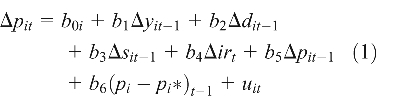
\begin{matrix} Δ p_{it} = & b_{0 i} + b_{1} Δ y_{it - 1} + b_{2} Δ d_{it - 1} \\ + b_{3} Δ s_{it - 1} + b_{4} Δ i r_{t} + b_{5} Δ p_{it - 1} \\ + b_{6} {(p_{i} - p_{i} *)}_{t - 1} + u_{it} \end{matrix}

(1)

The model captures the aforementioned features in a simple error-correction framework. In equation (1), the dependent variable is real housing price change (Δp) in city i in period t, while the explanatory variables include the one-period lagged deviation of housing prices from their long-run equilibrium level (p−p*), the previous period housing price growth, and changes in four fundamentals that may affect the short-run housing price dynamics based on the life-cycle model of the housing market (e.g. Meen, 2001). The four fundamentals can be seen as control variables in the model. The changes in real per capita income (y), population (d), and housing stock (s), are lagged to avoid potential endogeneity bias. This also allows for using the models for prediction purposes as long as the future change in real after-tax interest rate (ir) is predicted separately, since the influence of interest rate growth is allowed to be simultaneous. The model also includes a deterministic constant (b₀) that varies across cities. Since we use a nationwide measure for ir, we have dropped the subscript i from this variable.

A long-run equilibrium price level can be defined as one from which there is no systematic tendency to depart. Following Harter-Dreiman (2004), Holly et al. (2010), Lamont and Stein (1999) and Malpezzi (1999), among others, the long-run equilibrium housing price level in city i during period t is computed as the long-term relationship between real housing price level and real per capita disposable income:

p_{it}^{*} = δ_{i}^{*} y_{it}

(2)

The long-term coefficient on income (δ*) is allowed to vary across cities and differ from 1, since the equilibrium price-to-income ratio is not necessarily constant over time and space (see, e.g. DiPasquale and Wheaton, 1996; Malpezzi, 1999). Obviously, δ^* > 0.

Given that p and y are both non-stationary in levels but stationary in first differences (see the data section), we use the Johansen Trace test to test for cointegration between the variables. The Trace test works as a specification check for equation (2). The cointegration analysis is conducted and the long-run equilibrium relationship is estimated separately for each city. If the relationship in equation (2) is found to be stationary, i.e. p and y are pairwise cointegrated, and if the parameter δ* is found to be stable over time, then the relation can be regarded as one towards which housing prices tend to adjust and from which the price level cannot drift away in the long run. In this case, equation (2) can be interpreted as a long-term equation for housing prices, and additional fundamentals are not necessary in the empirical long-term equilibrium equation. The price level can temporarily deviate from p_t*, though. Instead, if cointegration could not be detected between housing prices and income, the relation could not be regarded as a long-run equilibrium relation for housing prices, implying that additional explanatory variables are necessary in equation (2).

In addition to the baseline model equation (1), we estimate fixed interaction-effects models that allow for different parameter estimates across cities or city groups:²

\begin{matrix} Δ p_{it} = & b_{0 i} + b_{1} Δ y_{it - 1} + b_{2} Δ d_{it - 1} \\ + b_{3} Δ s_{it - 1} + b_{4} Δ i r_{t} + b_{5 i} Δ p_{it - 1} \\ + b_{6 i} {(p_{i} - p_{i} *)}_{t - 1} + u_{it} \end{matrix}

(3)

\begin{matrix} Δ p_{it} = & b_{0 i} + b_{1} Δ y_{it - 1} + b_{2} Δ d_{it - 1} \\ + b_{3} Δ s_{it - 1} + b_{4} Δ i r_{t} + b_{5 j} Δ p_{it - 1} \\ + b_{6 j} {(p_{i} - p_{i} *)}_{t - 1} + u_{it} \end{matrix}

(4)

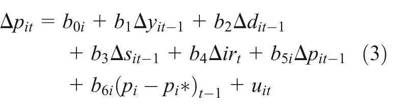
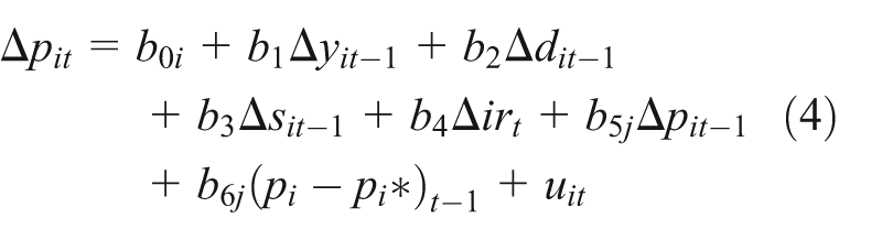
As our hypothesis concerns the regional variation in momentum and reversion dynamics, we let the momentum and reversion parameters vary across regions in equations (3) and (4). Specification (3) includes interaction dummies that allow the dynamics to vary across all 14 cities. Specification (4), in turn, allows the coefficients to differ between Helsinki, by far the greatest and most supply restricted city in Finland, and the other cities on aggregate (i.e. the slope coefficients are the same for all cities outside Helsinki). That is, j includes two ‘groups’: Helsinki and the other cities. To keep the models simple and to take advantage of the degrees of freedom gain provided by panel data, the parameters on control variables do not exhibit variation across cities in equations (3) or (4).

The sign of the speed of adjustment parameters (b₆) is expected to be negative: when the price level is higher than its long-run fundamental level, the price growth rate is expected to be small so that housing prices adjust towards their long-term equilibrium level. Given the notable frictions in the housing market and the potential backward-looking expectations, the momentum coefficient (b₅) is anticipated to be positive – fast housing price growth in this period predicts fast growth in the next period.

If the included fundamentals significantly affect the dynamics of Δp, the parameter signs are expected to be positive on Δy and Δd, and negative on Δir and Δs. If housing price dynamics are dominated by the momentum and reversion effects, the coefficients on the fundamentals may well be insignificantly different from zero, though.

A complication regarding a dynamic panel data model that includes the lagged dependent variable as an explanatory variable is endogeneity bias (Arellano and Bover, 1995; Blundell and Bond, 1998). Therefore, the panel models are estimated with the Arellano-Bover/Blundell-Bond estimator using the Generalised Method of Moments (GMM) technique, as this approach is designed for situation where the left-hand side variable is dependent on its own past realisations (see Arellano and Bover, 1995; Blundell and Bond, 1998). Compared with the ordinary least squares and two-stage least squares estimators, which are special cases of the linear GMM, the Arellano–Bover/Blundell–Bond estimator benefits from additional instruments that are orthogonal to the error term and are obtained from the lagged values of the potentially endogenous lagged dependent variable. This approach yields more unbiased estimates. A disadvantage of the Arellano–Bover/Blundell–Bond estimator is that it is quite complicated.

The two-period lagged transaction volume (total number of transactions) is used as the instrument for one-period lagged housing price change. The two-period lagged volume is used instead of the one-period lagged one, since transaction volume leads housing price movements. This is in line with previous empirical evidence for Finland (see Oikarinen, 2012), and with the theoretical considerations of e.g. Berkovec and Goodman (1996) and Hort (2000). In addition to the economic foundations for the relationship between housing prices and transaction volume, the instrument is highly correlated with the lagged price change (correlation is between 0.54–0.83 across cities, and 0.72 on average) and is exogenous to the dependent variable. Therefore, it is justifiable to consider the two-period lagged volume as a good instrument.

Furthermore, the estimated models may include spatial autocorrelation (Holly et al., 2010; Kuethe and Pede, 2011). Therefore, the Moran’s I test is conducted to investigate whether the models exhibit spatial autocorrelation. The test is conducted using several different ‘distance’ measures including the nearest neighbour distance, the number of inhabitants, distance from Helsinki, and various industry shares (as a proxy for the similarity of regions’ economic structures). Regardless of the distance measure, the test statistics do not show evidence of significant spatial autocorrelation.

Data

The empirical analysis is based on annual data for 14 Finnish cities for the period 1988–2012. The cities include the 10 largest in Finland and some other regional centres. It is reasonable to use data only since 1988, as the financial market deregulation that took place in Finland during the late 1980s induced a structural break in housing price dynamics (Oikarinen, 2009a, 2009b). The data are sourced from the Statistics Finland database unless mentioned otherwise.

The hedonic housing price indices computed by Statistics Finland measure the housing price development. The indices are based on transactions of privately financed apartments in the secondary market. There are good reasons to focus on the privately financed sector: in contrast with the publicly regulated (i.e. subsidised) sector, privately financed housing can be bought and sold at market prices without any restrictions. The data consist only of apartments, since data on apartments are more reliable than data on the other housing types: in Finland, apartments are a substantially more homogenous group than the other housing types, and a notably greater number of transactions take place in the apartment market than in the market for other housing types. That is, the use of apartment data diminishes the heterogeneity problem that is associated with housing price data even when hedonic indices are employed. As of 2012, the share of apartments of the total housing stock varied between 86% (Helsinki) and 45% (Kajaani) across the sample cities, and was 59% on average. This variation, too, can somewhat affect the observed dynamics.

The city-level income variable (y) is the after-tax per capita income of the city. Since the mortgage interest rates are practically the same all over the country, we use the nationwide after-tax mortgage rate to measure ir. The mortgage rate data are provided by the Bank of Finland. Finally, d is measured as city-level end-of-year population, and s as the end-of-year total housing stock (m²).

The panel models are estimated using real variables. Thus, p, y, and ir have been deflated by the cost of living index. Natural logs of all the variables except for the interest rate are used. There have been several changes in the administrational geographic boundaries of the cities after 2008. The data correspond to the city boundaries prior to those changes.

Table 1 presents summary statistics on housing price growth. All the housing price series are non-stationary based on the Augmented Dickey-Fuller (ADF) unit root test, while housing price growth is stationary. This is in line with previous empirical evidence reported for numerous housing markets. The unit root tests are applied individually for each city, since the cointegration tests are conducted separately for each city. All the other variables are difference stationary as well (these ADF test are available from the authors upon request). Table 1 also reveals that housing price growth is highly positively autocorrelated.

Table 1.

Descriptive statistics of real housing price growth.

City	Mean	SD	1st order autocorrelation	ADF level (lags)	ADF difference (lags)
Helsinki	0.015	0.112	0.478*	−1.01 (3)	−2.89** (0)
Tampere	0.010	0.094	0.523**	−1.63 (1)	−2.74** (0)
Turku	0.008	0.090	0.435*	−1.63 (1)	−3.21** (0)
Oulu	0.005	0.072	0.463**	−1.73 (1)	−2.49* (0)
Lahti	0.004	0.095	0.505**	−2.34 (1)	−2.91** (0)
Kuopio	0.009	0.093	0.445*	−1.93 (1)	−3.27** (0)
Jyväskylä	0.007	0.086	0.461*	−2.06 (1)	−3.08** (0)
Pori	0.010	0.085	0.481*	−2.12 (1)	−3.91** (0)
Lappeeranta	0.002	0.075	0.482*	−2.73 (1)	−3.10** (0)
Rovaniemi	0.008	0.085	0.506**	−2.26 (1)	−5.02** (3)
Vaasa	0.012	0.068	0.497*	−1.42 (1)	−2.95** (0)
Seinäjoki	0.010	0.087	0.196	−0.89 (0)	−4.32** (0)
Kotka	−0.005	0.090	0.638**	−1.45 (2)	−2.29* (0)
Kajaani	0.005	0.072	0.402*	−2.32 (1)	−3.38** (0)

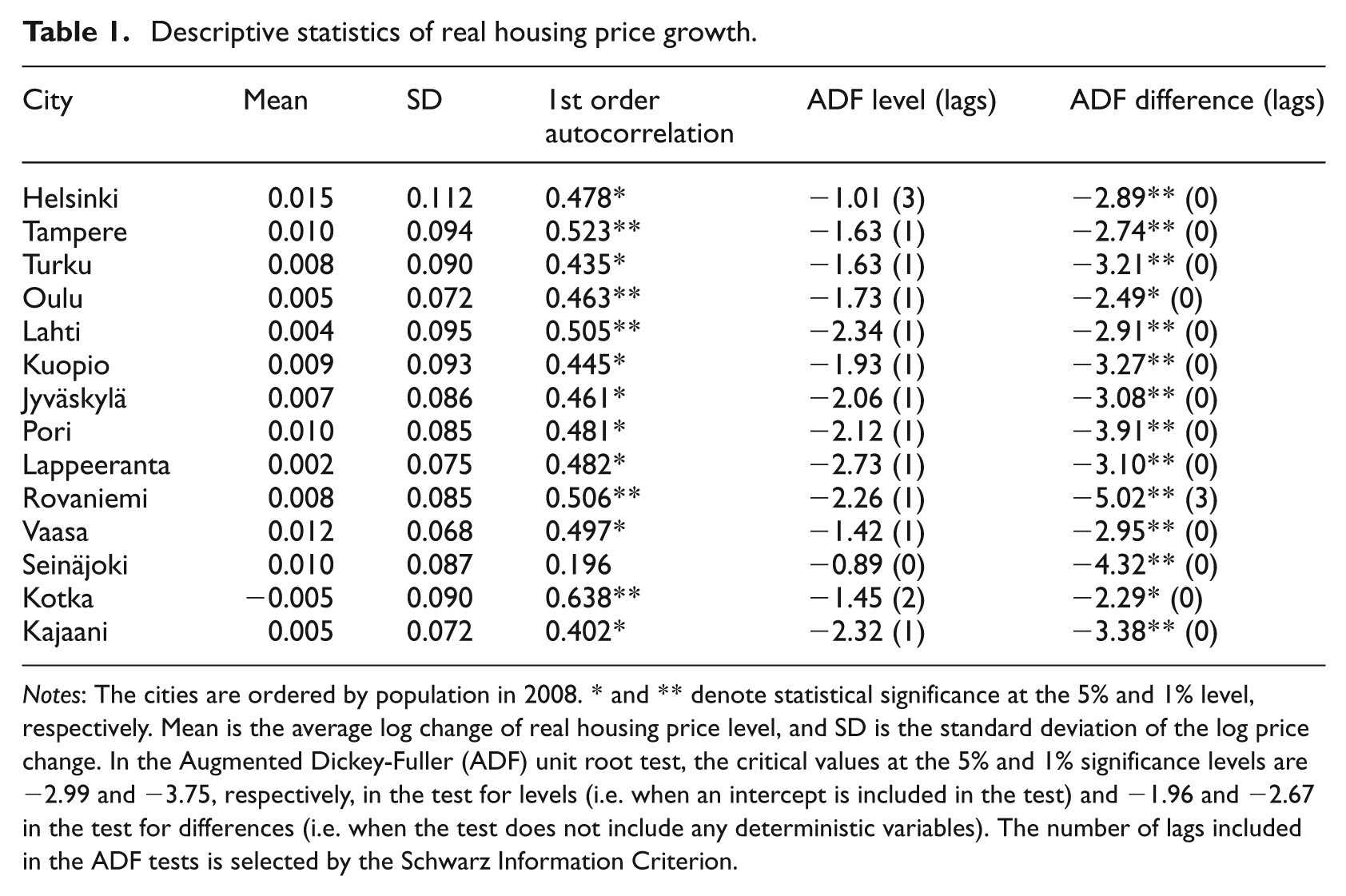
Notes: The cities are ordered by population in 2008. * and ** denote statistical significance at the 5% and 1% level, respectively. Mean is the average log change of real housing price level, and SD is the standard deviation of the log price change. In the Augmented Dickey-Fuller (ADF) unit root test, the critical values at the 5% and 1% significance levels are −2.99 and −3.75, respectively, in the test for levels (i.e. when an intercept is included in the test) and −1.96 and −2.67 in the test for differences (i.e. when the test does not include any deterministic variables). The number of lags included in the ADF tests is selected by the Schwarz Information Criterion.

Empirical results

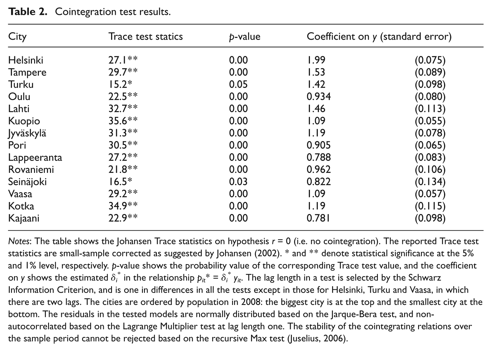
The Johansen Trace test results suggest that p and y are cointegrated in all the regions included in the analysis (Table 2). This is in line with the results by Malpezzi (1999) regarding the US. The cointegrating relations estimated by the Johansen Maximum Likelihood methodology are sensible with respect to the size of coefficients on y, and the stability of these relations cannot be rejected based on the recursive Max test (Juselius, 2006). Therefore, the long-term relations between p and y can be considered as reasonable measures for long-term equilibrium housing price levels in the cities.³

Table 2.

Cointegration test results.

City	Trace test statics	p-value	Coefficient on y (standard error)
Helsinki	27.1**	0.00	1.99	(0.075)
Tampere	29.7**	0.00	1.53	(0.089)
Turku	15.2*	0.05	1.42	(0.098)
Oulu	22.5**	0.00	0.934	(0.080)
Lahti	32.7**	0.00	1.46	(0.113)
Kuopio	35.6**	0.00	1.09	(0.055)
Jyväskylä	31.3**	0.00	1.19	(0.078)
Pori	30.5**	0.00	0.905	(0.065)
Lappeeranta	27.2**	0.00	0.788	(0.083)
Rovaniemi	21.8**	0.00	0.962	(0.106)
Seinäjoki	16.5*	0.03	0.822	(0.134)
Vaasa	29.2**	0.00	1.09	(0.057)
Kotka	34.9**	0.00	1.19	(0.115)
Kajaani	22.9**	0.00	0.781	(0.098)

Notes: The table shows the Johansen Trace statistics on hypothesis r = 0 (i.e. no cointegration). The reported Trace test statistics are small-sample corrected as suggested by Johansen (2002). * and ** denote statistical significance at the 5% and 1% level, respectively. p-value shows the probability value of the corresponding Trace test value, and the coefficient on y shows the estimated δ_i^* in the relationship p_it* = δ_i^* y_it. The lag length in a test is selected by the Schwarz Information Criterion, and is one in differences in all the tests except in those for Helsinki, Turku and Vaasa, in which there are two lags. The cities are ordered by population in 2008: the biggest city is at the top and the smallest city at the bottom. The residuals in the tested models are normally distributed based on the Jarque-Bera test, and non-autocorrelated based on the Lagrange Multiplier test at lag length one. The stability of the cointegrating relations over the sample period cannot be rejected based on the recursive Max test (Juselius, 2006).

The coefficient on y varies significantly across regions. In line with Malpezzi’s (1999) findings, the income elasticity of housing prices is greater in larger cities that are generally more supply-restricted because of the scarcity of vacant land in attractive sites. The coefficient is the greatest in the three biggest cities, and notably greater in Helsinki – by far the largest city – than in the second and third largest cities. Moreover, the income elasticity is the lowest in the smallest city (Kajaani). The simple correlation between the coefficient on y and population is as large as 0.83, while that between the coefficient on y and the price elasticity of housing supply (reported in Oikarinen et al., 2015) is −0.88. These correlations are as expected, since land leverage is generally smaller in the smaller and less supply restricted cities. That is, the correlations support the land leverage hypothesis. The land supply restrictions and land leverage are not the only factors affecting the coefficient, though (DiPasquale and Wheaton, 1996).

Figure 1 presents the evolution of real housing prices and their long-run fundamental level in the cities during 1988–2012. The graphs show clearly the price overshot in the late 1980s that followed the abolishment of financial market deregulation in Finland. After the price overshot, the dramatic drop in housing prices was strengthened by the deep recession in the Finnish economy during the early and mid 1990s.

Figure 1.

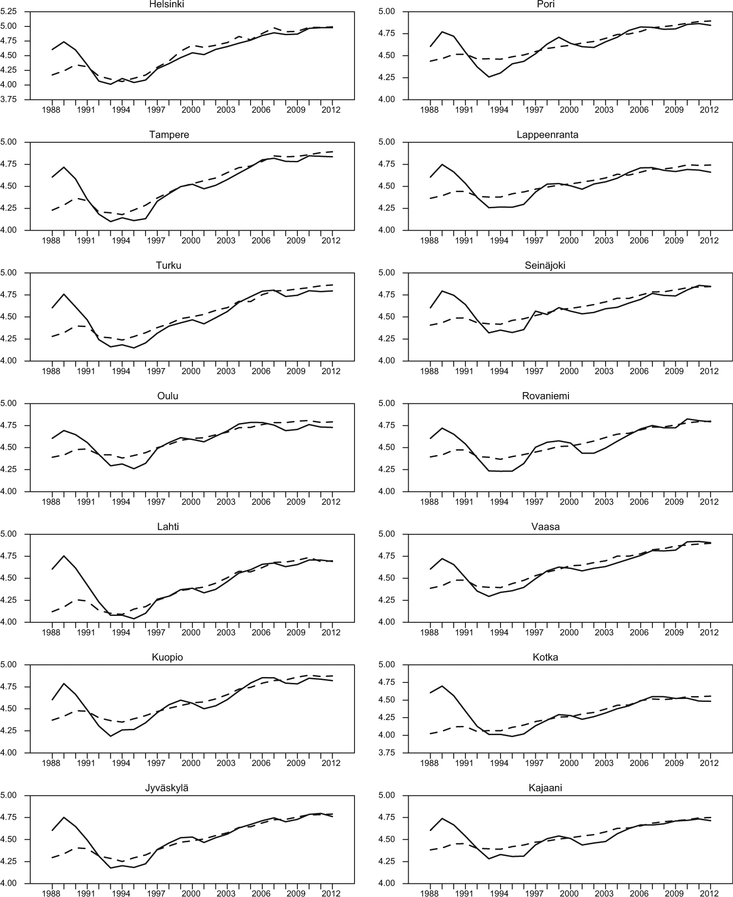
Real housing price indices and the long-run fundamental housing price level.

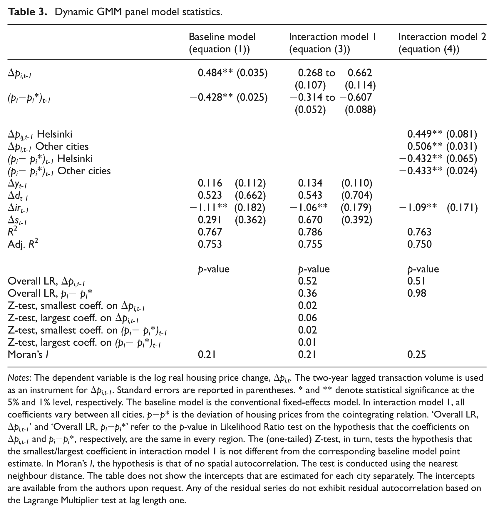
The deviations of observed housing price levels from the cointegrating relationships are used in the error-correction terms in the panel models. The dynamic GMM panel estimation results are presented in Table 3. The hypothesis of exogeneity of instruments is accepted by the Sargan test in all the presented models, and the Moran’s I test does not show evidence of spatial autocorrelation in any of the specifications. Hence, these models appear to be reasonably well specified.

Table 3.

Dynamic GMM panel model statistics.

	Baseline model (equation (1))	Interaction model 1 (equation (3))	Interaction model 2 (equation (4))
Δp_i,t-1	0.484** (0.035)	0.268 to 0.662
		(0.107) (0.114)
(p_i−p_i)_t-1*	−0.428** (0.025)	−0.314 to −0.607
		(0.052) (0.088)

Δp_ij,t-1 Helsinki			0.449** (0.081)
Δp_i,t-1 Other cities			0.506** (0.031)
(p_i− p_i)_t-1* Helsinki			−0.432** (0.065)
(p_i− p_i)_t-1* Other cities			−0.433** (0.024)
Δy_t-1	0.116 (0.112)	0.134 (0.110)
Δd_t-1	0.523 (0.662)	0.543 (0.704)
Δir_t-1	−1.11** (0.182)	−1.06** (0.179)	−1.09** (0.171)
Δs_t-1	0.291 (0.362)	0.670 (0.392)
R ²	0.767	0.786	0.763
Adj. R²	0.753	0.755	0.750

	p-value	p-value	p-value
Overall LR, Δp_i,t-1		0.52	0.51
Overall LR, p_i− p_i*		0.36	0.98
Z-test, smallest coeff. on Δp_i,t-1		0.02
Z-test, largest coeff. on Δp_i,t-1		0.06
Z-test, smallest coeff. on (p_i− p_i)_t-1*		0.02
Z-test, largest coeff. on (p_i− p_i)_t-1*		0.01
Moran’s I	0.21	0.21	0.25

Notes: The dependent variable is the log real housing price change, Δp_i,t. The two-year lagged transaction volume is used as an instrument for Δp_i,t-1. Standard errors are reported in parentheses. * and ** denote statistical significance at the 5% and 1% level, respectively. The baseline model is the conventional fixed-effects model. In interaction model 1, all coefficients vary between all cities. p−p* is the deviation of housing prices from the cointegrating relation. ‘Overall LR, Δp_i,t-1’ and ‘Overall LR, p_i−p_i*’ refer to the p-value in Likelihood Ratio test on the hypothesis that the coefficients on Δp_i,t-1 and p_i−p_i*, respectively, are the same in every region. The (one-tailed) Z-test, in turn, tests the hypothesis that the smallest/largest coefficient in interaction model 1 is not different from the corresponding baseline model point estimate. In Moran’s I, the hypothesis is that of no spatial autocorrelation. The test is conducted using the nearest neighbour distance. The table does not show the intercepts that are estimated for each city separately. The intercepts are available from the authors upon request. Any of the residual series do not exhibit residual autocorrelation based on the Lagrange Multiplier test at lag length one.

The estimated parameters generally have the expected sign and are of sensible magnitude. An exception is the positive point estimate on s in the baseline model and interaction model 1 (IM1). This estimate is not statistically significantly different from zero in either of the models, though. Some other control variables, too, are statistically insignificant. The point estimate on Δd_t-1, for instance, suggest that one percentage-point greater population growth this year predicts 0.5%-points faster housing price growth during the next year. One percentage-point faster interest rate growth, in turn, downgrades housing price growth by approximately one percentage-point.

Anyhow, we focus on investigating the momentum and reversion parameters, which have the expected signs and are statistically significant in each specification. In the baseline model (corresponding to equation (1) in the methodology section), the coefficient estimate 0.48 on Δp_t-1 indicates considerable momentum in housing prices: faster price growth this year predicts more rapid growth next year. The adjustment speed towards the long-run relation is somewhat faster than typically reported in the earlier related studies, the reversion coefficient being −0.43.

IM1, which corresponds to equation (3) and where the momentum and reversion coefficients are allowed to differ across all the 14 cities, shows notable regional variation in the dynamics: the momentum parameter ranges from 0.27 to 0.66 and the ‘bubble burster’ parameter from −0.31 to −0.61.⁴ This variation, overall, is not statistically significant based on the Likelihood Ratio (LR) test. However, the overall LR test statistics that study all the cities jointly are ‘diluted’ by the fact that for most cities the parameter estimates lie close to the mean value across all cities. In several cases there are statistically significant differences between two cities and, most importantly regarding our hypothesis, in a number of cases the city-specific parameter estimate on Δp_t-1 or on (p−p*)_t-1 differs statistically significantly from the corresponding point estimate of the baseline model. For instance, the smallest (Kotka) and largest (Kuopio) adjustment-speed estimates are statistically significantly different from the baseline model estimate. The same applies to the smallest (Seinäjoki) momentum estimate. The largest (Pori) momentum coefficient, too, differs from 0.484 at the 6% level of significance. This is a good example on how the ‘overall test’ can hide actual significant differences of some individual cities. Moreover, IM1 is preferred over the baseline model in terms of the model fit (adjusted R²). In sum, IM1 supports our hypothesis of significant regional differences in the dynamics.

Clearly, the differences indicated by IM1 are of economic significance as well.⁵ For instance, if housing prices were 20% below (above) their fundamental levels, the model would predict a 6%-point greater (smaller) housing price growth in Kuopio than in Kotka during the next year. A 5% price growth this year, in turn, would predict 2%-point faster price growth in Pori than in Seinäjoki.

Since Helsinki notably differs from the other cities in terms of size, but the other cities generally form a relatively uniform group, we further estimate a model that makes a distinction between Helsinki and the other cities (interaction model 2; corresponds to equation (4)). We also curtail this specification by dropping out the insignificant control variables. This makes the remaining point estimates more accurate and enhances the (adjusted) fit of the model.⁶ Despite the substantially greater size and considerably more inelastic housing supply in Helsinki than in the other cities (see Oikarinen et al., 2015), the results do not show evidence of different short-term dynamics in Helsinki compared with the rest of the cities. The estimates also closely correspond to those of the baseline model. This is not totally unexpected given the theoretical considerations presented above: while the informational factors suggest smaller momentum and faster reversion in Helsinki, the other structural factors – which generally concern the ability of housing supply to respond to changes in housing demand – propose just the opposite. It appears that in this case these factors cancel each other out.

The price dynamics are investigated in more detail in Figure 2. To show the impact of variation in the momentum parameter, in the upper-left and mid-left graphs the reversion coefficient is fixed to that of the baseline model, while the momentum parameter is allowed to vary between the smallest and largest point estimates from IM1. The upper-right and mid-right graphs, in turn, illustrate the influence of regional variation in the reversion parameter: while the momentum coefficient is assumed to equal that of the baseline model in all the curves, one curve is based on the maximum observed reversion speed and one is derived based on the minimum reversion coefficient from IM1. For comparison, all these four graphs show the adjustment path based on the baseline model too.

Figure 2.

Housing price adjustment paths.

The graphs in the upper part of Figure 2 assume an income change that increases the equilibrium housing price level by 1%, i.e., an income growth of approximately 0.5%−1.3% depending on the city. The graphs in the mid part show the housing price evolution after 1% increase in the housing price level that is not accompanied with a change in the income. These graphs show that regional variation in the momentum effect, in particular, has notable effects on the dynamics. For instance, the price peak caused by the equilibrium level growth is almost 40% higher in the greatest momentum case than in the smallest momentum city, and almost 20% higher (smaller) in the most (least) prominent momentum case than implied by the baseline model (upper-left graph). The variation in momentum also considerably affects the oscillation of prices around the equilibrium price level. The differences in reversion parameter, in turn, have an effect on the reaction speed to changes, especially: the greater is the reversion parameter, the faster is the price reaction.

The low part of Figure 2 presents the response of housing prices to 1% increase in income. The lower-left graph is based on the short-term parameters from the baseline model, while allowing the long-term income elasticity to vary across the two cities – Helsinki with the largest elasticity and Kajaani with the smallest one. Clearly, the long-term income elasticity has a substantial influence on the price development. Finally, based on IM1, the lower-right graph compares the housing price adjustment in Helsinki to that in Kuopio, whose point estimates 0.65 on Δp_t-1 and −0.61 on (p−p*)_t-1 notably differ from the baseline model and from those estimated for Helsinki (0.44 and −0.44, respectively). This graph also includes curve for Kuopio that is based on the baseline model estimates. Among other differences, the estimates from IM1 suggest an approximately 40% greater impact on prices in Kuopio at the two-year horizon than the baseline model would predict.

Overall, Figure 2 shows that the kind of differences that we find regarding the long- and short-term parameters can have considerable influences on regional housing price dynamics, and that assuming similar dynamics across cities can yield misleading conclusions and forecasts. It also is good to keep in mind that the possibly notable differences in the development of fundamentals across cities, too, may cause substantial regional differences in the housing price development.

Note that there is a tendency of housing prices to oscillate around the long-run fundamental level in the largest momentum and reversion cases and, to a lesser extent, based on the baseline model, i.e. in the cities on average. This feature resembles dynamics in the ‘Region III’ derived in Capozza et al. (2004). Capozza et al. (2004) show that oscillatory convergence generally characterises housing price dynamics in the US metro areas too.

Interestingly, the city-specific momentum parameters (IM1) have large and statistically significant negative correlations with the population density and transaction volume of the market. This is in line with the considerations of Clapp et al. (1995), Hirshleifer et al. (2013) and Kumar (2009) that emphasise the role of information flows on asset price dynamics. The reversion parameter, instead, is not notably correlated with the density or transaction volume, and neither of the parameters is correlated with the supply elasticity of housing.

Finally, note that the greater tendency of housing prices to oscillate around the long-run relationship in a given city does not necessarily imply that prices are expected to be more volatile in that city, at least in the long run. This is clearly illustrated by the lower-right part of Figure 2: 1% income growth yields a much greater eventual price change in Helsinki than in Kuopio. In the long-run, it is the long-term price elasticity with respect to demand factors that dominates the price volatility.

Conclusions

This study aims is to examine empirically the magnitude of regional differences in housing price dynamics using panel data models. We hypothesise that there are significant regional differences in the momentum effect of housing prices (‘bubble builder’), in the reversion speed of housing prices towards their long-run fundamental level (‘bubble burster’), and in the long-term elasticity of housing prices with respect to income. The study contributes to the literature by being the first one that allows for regional variation in both the long-term and short-term housing price dynamics and where the significance of differences in the momentum and equilibrium-adjustment parameters is tested formally in a panel framework. This also is one of the very few studies on housing price dynamics allowing for regional differences in a panel setting that is not based on US data. The analysis can be seen as a test for the validity of the conventionally used panel data models that assume the housing price dynamics to be the same across all the housing markets included in the model.

Applying the Arellano–Bover/Blundell–Bond GMM technique for a panel of 14 Finnish cities, the regional differences in short-run housing price dynamics are found to be relatively small, overall. Nevertheless, in a number of cities either the momentum or reversion parameter differs significantly from that of the baseline model which does not allow for regional variation. Moreover, the long-run coefficient on income substantially varies across regions. Thus, although the regional variation in the short-term dynamics generally is relatively small, the results support our hypothesis and indicate that the use of the conventional models that assume similar dynamics across regions can result in misleading conclusions.

The results are in line with a hypothesis according to which the informational factors have a more significant impact on the short-term momentum dynamics than the supply restrictions do: the momentum effect generally is smaller in the cities with higher population density and greater number of housing transactions. Furthermore, the analysis provides support for cointegration between housing prices and income. In general, the long-term coefficient on income is the greater, the larger and more supply restricted is the city, as expected.

This empirical analysis is conducted using data for a country that is relatively small in size and coherent in terms of culture and income. In a geographically larger and culturally and economically more diverse country than Finland, the regional differences are likely to be more pronounced, making the panel models that do not allow for regional differences in the dynamics even more complicated than indicated by this study. Therefore, further empirical examination on the extent of regional differences in the housing price dynamics using panel data methods for other countries is desirable.

Footnotes

Acknowledgements

We are grateful to three anonymous referees for their constructive comments. The article also benefited from discussions at the 19th Annual Conference of the European Real Estate Society in Edinburgh (UK), at the 53rd European Regional Science Association Conference in Bratislava (Slovakia), and at the Finnish Economic Association XXXV Annual Meeting in Vaasa (Finland), and from comments by Mika Haapanen and Juha Junttila. The usual disclaimer applies.

Funding

Funding was received from the Academy of Finland (decision number 268310); Kluuvi Foundation; OP-Pohjola Group Research Foundation.

Notes

References

Abraham

Hendershott

(1996) Bubbles in metropolitan housing markets. Journal of Housing Research 7(2): 191–207.

Arellano

Bover

(1995) Another look at the instrumental variable estimation of error-components models. Journal of Econometrics 68(1): 29–51.

Blundell

Bond

(1998) Initial conditions and moment restrictions in dynamic panel data models. Journal of Econometrics 87(1): 115–143.

Beracha

Skiba

(2011) Momentum in residential real estate. Journal of Real Estate Finance and Economics 43(3): 299–320.

Berkovec

Goodman

(1996) Turnover as a measure of demand for existing homes. Real Estate Economics 24(4): 421–440.

Bostic

Longhofer

Redfearn

(2007) Land leverage: Decomposing home price dynamics. Real Estate Economics 35(2): 183–208.

Bourassa

Haurin

. (2009) House price changes and idiosyncratic risk: The impact of property characteristics. Real Estate Economics 37(2): 259–278.

Bourassa

Hoesli

Scognamiglio

. (2011) Land leverage and house prices. Regional Science and Urban Economics 41(2): 134–144.

Bramley

Leishman

(2005) Planning and housing supply in two-speed Britain: Modelling local market outcomes. Urban Studies 42(12): 2213–2244.

10.

Capozza

Hendershott

Mack

(2004) An anatomy of price dynamics in illiquid markets: Analysis and evidence from local housing markets. Real Estate Economics 32(1): 1–32.

11.

Case

Shiller

(1989) The efficiency of the market for single-family homes. American Economic Review 79(1): 125–137.

12.

Case

Shiller

(1990) Forecasting prices and excess returns in the housing market. Real Estate Economics 18(3): 253–73.

13.

Clapp

Dolde

Tirtiroglu

(1995) Imperfect information and investor inferences from housing price dynamics. Real Estate Economics 23(3): 239–269.

14.

Davis

Heathcote

(2007) The price and quantity of residential land in the united states. Journal of Monetary Economics 54(8): 2595–2620.

15.

DiPasquale

Wheaton

(1996) Urban Economics and Real Estate Markets. Englewood Cliffs, NJ: Prentice Hall.

16.

Dusansky

Koç

(2007) The capital gains effect in the demand for housing. Journal of Urban Economics 61(2): 287–298.

17.

Englund

Ioannides

(1997) House price dynamics: An international empirical perspective. Journal of Housing Economics 6(2): 119–136.

18.

Glaeser

Gyourko

Saiz

(2008) Housing supply and housing bubbles. Journal of Urban Economics 64(2): 198–217.

19.

Gyourko

Saiz

(2006) Construction costs and the supply of housing structure. Journal of Regional Science 46(4): 661–680.

20.

Harter-Dreiman

(2004) Drawing inferences about housing supply elasticity from house price responses to income shocks. Journal of Urban Economics 55(2): 316–337.

21.

Hirshleifer

Hsu

(2013) Innovative efficiency and stock returns. Journal of Financial Economics 107(3): 632–654.

22.

Holly

Pesaran

Yamagata

(2010) A spatio-temporal model of house prices in the USA. Journal of Econometrics 158(1): 160–173.

23.

Hort

(2000) Prices and turnover in the market for owner-occupied homes. Regional Science and Urban Economics 30(1): 99–119.

24.

Hwang

Quigley

(2006) Economic fundamentals in local housing markets: Evidence from U.S. metropolitan regions. Journal of Regional Science 46(3): 425–453.

25.

Johansen

(2002) A small sample correction for the test of cointegrating rank in the vector autoregressive model. Econometrica 70(5): 1929–1961.

26.

Jud

Winkler

(2002) The dynamics of metropolitan housing prices. Journal of Real Estate Research 23(1): 29–46.

27.

Juselius

(2006) The Cointegrated VAR model: Methodology and Applications. Oxford: Oxford University Press.

28.

Kuethe

Pede

(2011) Regional housing price cycles: A spatio-temporal analysis using US state-level data. Regional Studies 45(5): 563–574.

29.

Kumar

(2009) Hard-to-value stocks, behavioral biases, and informed trading. Journal of Financial and Quantitative Analysis 44(6): 1375–1401.

30.

Lamont

Stein

(1999) Leverage and house-price dynamics in U.S. cities. Rand Journal of Economics 30(3): 498–514.

31.

Malpezzi

(1999) A simple error correction model of house prices. Journal of Housing Economics 8(1): 27–62.

32.

Meen

(2001) Modelling Spatial Housing Markets: Theory, Analysis and Policy. Massachusetts, MA: Kluwer Academic Publishers.

33.

Oikarinen

(2009a) Household borrowing and metropolitan housing price dynamics – Empirical evidence from Helsinki. Journal of Housing Economics 18(2): 126–139.

34.

Oikarinen

(2009b) Interaction between housing prices and household borrowing: The Finnish case. Journal of Banking & Finance 33(4): 747–756.

35.

Oikarinen

(2012) Empirical evidence on the reaction speeds of housing prices and sales to demand shocks. Journal of Housing Economics 21(1): 41–54.

36.

Oikarinen

Peltola

Valtonen

(2015) Regional variation in the elasticity of supply of housing, and its determinants: The case of a small sparsely populated country. Regional Science and Urban Economics 50(1): 18–30.

37.

Røed Larsen

Weum

(2008) Testing the efficiency of the Norwegian housing market. Journal of Urban Economics 64(2): 510–517.

38.

Wilhelmsson

(2008) Regional house prices: An application of a two-equation model to the Swedish housing market. International Journal of Housing Markets and Analysis 1(1): 33–51.