Measuring the influence of space and time effects on time on the market

Introduction

Time on the market (TOM) has been considered by many authors as a leading indicator of the housing market with variations in TOM, lengthening or shortening in duration, occurring in advance of changes in either sale price or asking price observed. Various studies over the past decades have sought to link TOM with sale price and liquidity in the housing market. Miller (1978) showed that TOM varied according to buyer and seller reactions to different market conditions. Two decades later Kramer (1999) considered how housing demand, the housing cycle, liquidity and seller behaviour impacted on the decision to sell. McGreal et al. (2009) explored lead-lag relationship between asking prices, sale prices and TOM while Haurin et al. (2013) discussed significant and substantial responses to marketing time for boom and bust periods. However, most studies have focused upon the relationship of TOM with various property characteristics, for example Haurin (1988) showed how atypicality may increase the selling period for a property.

This paper takes a different perspective and seeks to analyse the extent to which TOM for any individual property is influenced by spatial dependence or interaction with neighbouring properties. Previous research has shown that spatial dependence and spatial auto-correlation occur in house prices (Basu and Thibodeau, 1998) but there has been an absence of any equivalent research in relation to the extent that TOM is influenced by spatial effects. The a priori expectation is that a dwelling located in a neighbourhood with a less buoyant housing market exhibits higher TOM than a similar property located in a higher demand neighbourhood, the inference being that spatial clustering of TOM may occur arising from specific characteristics relating to the quality of dwellings (Haurin, 1988) and the neighbourhood/submarket in which dwellings are located (Pryce and Gibb, 2006), making the separation of effects complex. However, to date, there is no empirical analysis that has examined spatial effects of TOM to support whether such a hypothesis regarding clustering is observable, though Anglin et al. (2003) in articulating the complexity of market behaviour argued that TOM varies more with spatial location and market conditions than it does with property characteristics.

Given this context, the paper seeks to address this gap in the literature base, the originality of the study stemming from an analysis of whether TOM is distributed randomly across an urban area or whether there are spatial effects embedded in TOM and, if the latter are observable, how are such spatial effects influenced by time effects. Understanding of these complex space-time influences and their impact on TOM arguably leads to a better appreciation of the dynamics underpinning the operation of housing markets (McGreal and Taltavull, 2013).

The empirical research underpinning this paper relates to the metropolitan area of Adelaide (South Australia), population 1.3 million, for which an extensive database of house sales transactions has been developed. Prior research (Rossini et al., 2012) has suggested the existence of a number of spatial housing sub-markets within this metropolitan area which extends for over 100 km from north to south but is constrained geographically by the sea to the west and the Adelaide Hills to the east.

The paper is structured as follows. The second section provides a reflection on some of the leading literature on TOM for residential property highlighting the relative lack of spatial analysis of TOM. The third section outlines the data underpinning the study. In the fourth section the initial analysis is concerned with testing for spatial autocorrelation in TOM globally using Moran’s I and locally using LISA (Local Indicator of Spatial Association) models. The fifth section extends the analysis using a 2SLS STAR model to analyse space-time effects. In the sixth section conclusions are drawn.

TOM: Literature review

The literature on TOM has been predominantly from the US with early studies stemming from the 1970s (Belkin et al., 1976; Cubin, 1974; Miller, 1978) primarily focusing on differences between list price, sale price and the impact of time on selling price. Later studies developed these relationships further using larger sample sizes and more rigorous modelling of TOM, such as the work by Anglin et al. (2003) who examined how over-pricing influenced TOM. More recent research on TOM has extended beyond the US to, for example, studies in the UK (Levin and Pryce, 2007; McGreal et al., 2009; Pryce and Gibb, 2006), and other European countries such as the study by Bjorlkund et al. (2004) in Sweden.

The consensus of most of the ensuing studies has been that TOM impacts on selling price, though the direction of this impact has caused some debate. According to Taylor (1999), a longer TOM should produce a higher selling price as over time the greater is the probability of attracting a buyer with a high reservation price. Likewise Forgey et al. (1996) argued that higher selling prices were associated with longer expected selling periods while Asabare et al. (1993) also concluded that the longer the marketing period the greater the probability that a higher price can be achieved. Voicing a different perspective, Larsen and Park (1989) concluded that, all things being equal, the longer a property is on the market the greater is the concession in terms of price. Sirmans et al. (2005) also suggest that in many situations TOM has a negative influence on price and Taylor (1999) conceded that a house which has been on the market for a long time may acquire a stigma with reduced pricing a result. Haurin (1988) showed that atypicality in a property can produce a longer TOM with longer selling time for a property with unusual characteristics relative to a standard property. Levin and Pryce (2009) argued that a seller’s decision to wait for an extra bid may raise expected selling price due to more potential buyers but, on the downside, they showed that diminishing returns may result from the costs of holding including financing and depreciation. Kramer (1999) focused on the liquidity aspects of TOM suggesting that when housing demand is high sellers do not in fact raise their prices to take full advantage rather they look for greater liquidity so as to complete the sale before the market ‘turns on them’. Alternatively in periods when market demand is low, Kramer argued that sellers do not drop their prices in order to achieve the same amount of liquidity as in the boom market. Haurin et al. (2013), using data from the Belfast (Northern Ireland) housing market, have demonstrated how TOM varied across the most recent housing market cycle. Their analysis showed that in the stable market period (2002Q1 to 2005Q2) TOM averaged 102 days but during the boom (2005Q3 to 2007Q3) mean TOM fell to 50 days and rose to 179 days in the recession. Using a proportional hazards model, they established that unexpected (short duration) price shocks change the duration of the marketing time, with a positive demand shock resulting in rising prices and reducing TOM.

Several studies have sought to identify the factors which influence TOM. TOM has been explained by quantifiable factors such as property characteristics, including dwelling type and characteristics (Haurin, 1988), age (Kang and Gardner, 1989; McGreal et al., 2009), quality and size (Forgey et al., 1996; Jud et al., 1996; Taylor, 1999), market conditions including interest rates and employment (Kalra and Chan, 1994), as well as qualitative factors such as agency performance (Gwin et al., 2002; Jud et al., 1996; Sirmans et al., 1991), seller motivations (Genesove and Mayer, 1997; Glower et al., 1998; Springer, 1996), regulation and by the types of buyer operating in different market conditions (Brown et al., 2013).

In comparison, few studies have focused on how TOM might vary spatially or be influenced by a combination of space-time effects. Anglin et al. (2003) make an important contribution to this debate in identifying that TOM varies by spatial location and market conditions. With reference to the Glasgow (Scotland) housing market, Pryce and Gibb (2006) concluded that booming markets tend to have an early peak in the hazard function followed by a steep decline. They also showed a spatial effect with the TOM hazard function varying across Glasgow which they interpreted as evidence of submarkets. Beyond this inference, Pryce and Gibb did not extend their study into the field of spatial analysis though their work is of significance to this paper in highlighting duration dependence in TOM and shifts in that dependence over time and space. A study by Rossini et al. (2012) of the Adelaide market over a three month period also examined the impact of location on TOM using hazard models. These models supported the proposition that, holding other variables constant, dwelling size together with location were major factors in determining time on market. Generally smaller houses located close to the city centre had the shortest time on market while larger properties, at some distance from the city centre, had the longest time on market. Although the hazard models indicated that TOM was fundamentally related both to size of property and to location, regardless of dwelling type, no further spatial modelling was attempted.

In summary the existing literature provides a useful foundation to the analysis undertaken in this paper but does not provide any direct comparator papers. The innovative nature of this paper is the consideration of whether there are spatial effects embedded in TOM, how these spatial effects are, in turn, influenced by time effects and how unobservables, as measured by spatial error, can impact on TOM.

Data

This study is based on residential property transactions in the metropolitan area of Adelaide, South Australia over the period from January 2002 to December 2011, a total of 40 quarters. Adelaide, with a population of 1.3 million, is the fifth largest city in Australia by size and has an economic structure strongly based on industry and services. With its relative geographical isolation, clearly defined by urban growth boundary, and minimum external market influences Adelaide provides an ideal case study. The metropolitan area which contains over 300 suburbs of variable sizes and around 100 postal (zip) codes constitutes 10 geographical sub-divisions (Figure 1). Established in a previous study (Rossini et al., 2005), these have been used for indexing the Adelaide housing market with the spatial groupings formed from contiguous postcodes and based on a combination of socio-economic and physical criteria.

OPEN IN VIEWER

Figure 1.

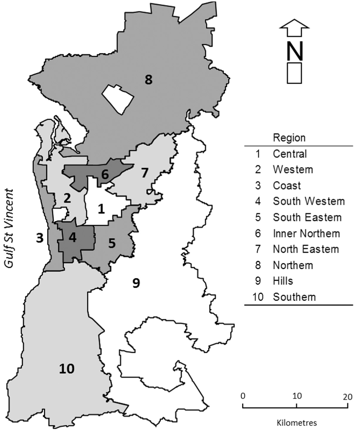
Geographical sub-division, Adelaide Metropolitan Area.

Adelaide’s economy has for decades been strongly aligned with manufacturing and thus has felt the effects of the prolonged period of a high Australian dollar (Government of South Australia, 2013). The mining sector of South Australia is in an earlier stage of development than in states such as Western Australia and Queensland and to this extent has not been exposed to the more volatile economic conditions of comparable Australian cites such as Perth and Brisbane. Over the period of the study, the state of South Australia averaged economic growth of 2.8% (Government of South Australia, 2013) close to the Australian average of 3.2% and Adelaide, in line with other Australian cities, did not encounter a substantial downturn in its housing market during the Global Financial Crisis (GFC). Instead house prices across the Australian market, between 2002 and 2011, consistently trended upwards with median prices for detached dwellings increasing on average by 127% (ABS, 2014). Over this period Perth and Brisbane showed annualised median price increases of 10.9% and 10.3% respectively, reflecting the boom in the mining sector, with Adelaide’s annualised price rise of 9.4% comparing favourably. In comparison, price rises in Australia’s largest cities such as Melbourne (7.5%) and Sydney (4.2%) were more subdued. In 2009, as a late response to the GFC, there was a temporary slowing in house price rise across Australia with falls in Sydney (-0.5%), Perth (-2%) and Brisbane (-1%). In 2009 median house prices fell in Adelaide by 0.5% (ABS, 2014). However, this effect was short-lived and in 2010 house prices in every sector of the Australian market, including Adelaide, began again to trend upwards, largely as a result of a significant fall in mortgage rates. Thus throughout the period of the study house price trends in Adelaide largely replicated those of other housing markets in Australia (ABS, 2014) and hence the market dynamics in Adelaide can be considered as reflective of other cities.

Likewise, in terms of the marketing process, most housing in Adelaide is sold through a real estate agent based on commission similar to the practice used in the UK and USA. Most properties will sell with a sole agency agreement (exclusive right for that agent) where the agent advertises the property for sale and seeks bids from potential purchasers who may then negotiate on the final price (Cucchiarelli and McGreal, 2012). A small percentage of properties are auctioned and these are usually either unique properties or sales of estates or foreclosed properties. Properties advertised for auction can sell prior to auction, at the auction or through a private negotiation after the auction. A very small percentage of houses are sold by tender. Thus in terms of marketing residential property, Adelaide is typical of processes followed both in other Australian cities and internationally, thus findings from this paper concerning TOM and the spatial/temporal analysis undertaken has application beyond the confines of the specific case study.

The dataset that underpins the analysis in this paper was assembled by searching the sales history file complied by the State Government of South Australia for relevant transactions and cross referencing these against online information from RPdata, the largest commercial provider of real estate data in Australia. RPdata captures all advertised property either at the point of appearing in newspapers or once weekly from RealEstate.com, a national Australian real estate advertising site, which is extensively used in South Australia. Dates and advertisement details (including indicated prices) are recorded. To standardise the analysis and reduce variability that may arise from different property types, only detached residential properties, the predominant dwelling type in Adelaide, (77.2% based on the 2011 Australian census) are considered in this analysis. Although in a previous study of the Adelaide housing market (Rossini et al., 2012) survival functions used to predict TOM were almost identical for different types of housing, a strong locational bias for non-detached housing across the Adelaide metropolitan area could influence the results of this study. Thus for the purposes of the modelling and analysis underpinning this paper it was decided to hold housing type constant. Furthermore, in addition to being the dominant property type, the location of detached dwellings is well distributed across the geographical area with significant representation in all sub-markets and also over time in terms of the volumes of sales activity.

Regarding data quality, all properties that have been settled in the Lands Title Office (LTO) appear on the State Government’s sale history file. The information recorded includes the sale price, non-market sales indicators, ¹ the date of settlement from the LTO, dwelling descriptors, site and capital values from the Valuer General’s office. The dataset used in this research extracted only market transactions of detached residential houses from the sales history file and then individually interrogated the online RPdata market history to determine TOM. Time on market is counted as the number of days between the first and the last advertised date. This is recoded for all residential properties ‘on the market’ which is RPdata’s primary source of data. The actual settlement date of the transaction is not used. This triangulation of these sources has ensured an accurate and robust dataset upon which the analysis is based. In total, 120,489 records were matched ² representing over 65% of all market transactions of detached residential properties over the study period. Finally each of these records was geo-coded with coordinates based on address allowing analysis at an individual property level.

The market for detached houses within metropolitan Adelaide has experienced significant changes over the period of this study (Figure 2). TOM was at its shortest duration through 2002 and early 2003 associated with periods of high sales volumes and price increases. Thereafter, prices stabilised with a decrease in the volume of detached sales from 2004 to 2007 and a large increase in average TOM. In the six months immediately prior to the GFC in mid-2007, the detached housing market in Adelaide experienced an upswing with increased sales volumes and prices and lower TOM. The slower market in 2008, the only occurrence of negative growth within the period (2002–2011), was accompanied by a subsequent decrease in the volume of transactions and an increased TOM. However, a number of post GFC Government incentives saw the market improve for a short period during 2009 and early 2010 although transactions volumes remained lower and TOM decreased only marginally. By the end of 2011 the market showed some recovery in sales volumes but with lower prices and TOM increasing to its highest level over the study period.

OPEN IN VIEWER

Figure 2.

Median TOM and percentage change in median price.

Table 1 provides summary statistics for the study period, 2002 to 2011. The mean and median transaction prices of AUS$368,770 and AUS$320,000 respectively indicate a peaked and positively skewed distribution. Mean TOM is 52.43 days (median TOM 29.00 days). The TOM distribution is less peaked than price (kurtosis is 5.11, compared to 42.87 for sale price) and less skewed (2.04 compared to 4.34 for sale price). Using the 10 sub-divisions identified for the Adelaide housing market (Rossini et al., 2005), median TOM suggests appreciable spatial variation across the metropolitan area and also by time over the period 2002 to 2011. This pattern of variation in TOM forms the basis of the analysis in the subsequent sections of this paper.

OPEN IN VIEWER

Table 1.

Descriptive analysis, median TOM by location and year.

Location	2002	2003	2004	2005	2006	2007	2008	2009	2010	2011
Central	15	15	22	22	22	22	29	50	29	45
Western	15	15	22	36	29	23	29	42	32	58
Coast	15	15	22	36	29	23	30	50	34	59
South Western	15	15	22	22	22	20	26	37	29	51
South Eastern	22	15	22	29	28	22	33	44	36	57
Inner Northern	15	15	22	36	29	22	29	47	33	49
North Eastern	15	8	22	36	31	22	37	49	36	61
Northern	8	8	29	50	50	31	45	51	52	80
Hills	15	15	30	50	43	32	43	60	49	73
Southern	8	8	27	36	30	21	34	43	43	65

Spatial autocorrelation in TOM

Estimation of spatial correlation necessitates the determination of spatial dependence or spatial lag, namely the relationship between property ‘i’ with the other properties ‘j’ in its proximity (with j ≠ i). Spatial interaction exists due to observed or unobserved heterogeneity in the spatial structure, known as spatial heterogeneity or spatial error (Anselin, 1988). According to Anselin, setting aside measurement problems, the spatial structure of phenomena generates complex patterns of interaction which can be multidirectional in nature. It is this dependency and the extent that it exists within TOM data that is the central concern of this paper.

As discussed by McGreal and Taltavull (2013) different econometric techniques, including STAR models (Anselin, 1999) have been developed to control for spatial dependence. STAR models consider that both geographical and time dependences can be parameterised in a matrix W which captures the spatial relations between pairs of observations as well as time dependence ((Anselin, 1998). To estimate the spatial effects, this paper has developed spatial matrices based on both distance (Euclidean) and contiguity following the algorithm of Anselin and Smirnov (1996). While the authors recognise the limitations that characterise spatial analysis, these are reduced by the existence of latitude and longitude coordinates for each property working within the boundaries of the geographical sub-markets previously identified for Adelaide (Figure 1). Initially a four W matrix was developed using order 1 of contiguity (Rook and Queen matrices) and a 4-nearest neighbours distance matrix. Thereafter, for subsequent iterations, the matrix was based on the Queen design only as it considers boundaries as well as vertices of a symmetric matrix and thereby provides the possibility of building a more complete matrix. ³ Moran’s I as a measure of global spatial autocorrelation in the data was used to measure the extent to which points that are ‘close together’ in space have, on average, similar values. Moran’s I also measures the extent to which variables are clustered by value.

Estimations of spatial autocorrelation for TOM (univariate analysis) show a small spatial lag interaction, with a Moran’s I stat = 0.0896558 indicating that an incremental increase of one day in TOM in location ‘i’ is associated with an additional 0.089 days on average for a property close to the subject property. The low correlation suggests the spatial pattern for TOM to be mostly random with the null hypothesis of no spatial clustering of TOM not rejected. To test these outcomes, we re-estimate Moran’s I increasing the density of the spatial matrix to a 300 nearest neighbours W-matrix finding a similar result, with the value of the Moran’s I statistic declining to 0.032 and reinforcing the lack of any significant pattern at a global level within the TOM dataset. Similar results were obtained for different sizes of the W matrix and are contrary to the perception of clustering in TOM, as suggested by the descriptive analysis of TOM for the 10 geographical sub-divisions in Adelaide (Table 1).

As TOM has been shown to vary across the housing cycle (see e.g. Haurin et al., 2013), the analysis considered the consistency of local Moran’s I or Local Indicator Spatial Association (LISA) models using sub-sets of the data to reflect properties listed and sold in each calendar year (Table 2). Such models provide an indication of spatial clustering of similar or dissimilar values around an individual observation giving a measure of how correlated a value is with surrounding measurements. The analysis at an annual level produces similar results to the full dataset with each year showing a small spatial lag and suggesting close to a random effect. Indeed there is a high level of consistency in the results across the cycle with little variation apparent. While the volume of sales, as expected, varies appreciably reflecting the differing market dynamics the analysis indicates for most observations (repeatedly averaging at circa 86% per annum) TOM is not significant and not spatially clustered. Extracting the listed but unsold properties by year, the Moran’s I estimated for each of these sub-samples likewise gives small values suggesting that these unsold properties are also randomly distributed across space with no clustering evident at a local level (Table 2).

OPEN IN VIEWER

Table 2.

Local Moran’s I LISA analysis by year for sold properties and listed but not sold properties (significance level 0.05).

Year	Sold properties					Listed properties
	# significant	Local Moran’s I	# insignificant	Percentage insignificant	Spatial distribution	Local Moran’s I	Spatial distribution
2002	8070	0.034792	7009	86.85%	random	0.027943	random
2003	8034	0.045743	6929	86.25%	random	0.038915	random
2004	12,549	0.029586	11,123	88.64%	random	0.038915	random
2005	12,785	0.049134	11,021	86.20%	random	0.053455	random
2006	13,636	0.058851	11,617	85.19%	random	0.023091	random
2007	15,001	0.055626	12,910	86.06%	random	0.07055	random
2008	13,137	0.064097	11,302	86.03%	random	0.043073	random
2009	14,090	0.056522	12,129	86.08%	random	0.018473	random
2010	10,556	0.036344	9172	86.89%	random	0.041374	random
2011	11,590	0.054523	9970	86.02%	random	0.047637	random

The remainder of the observations show that some localised clusters of High-High TOM are scattered throughout the metropolitan area, associated with less dynamic sub-markets and Low-Low TOM focused on sub-markets associated with the central locations of the city and indicative of more dynamic sub-markets in terms of transactions. The outcome of the LISA analysis indicates that in the vast majority of cases there are no spatial interaction effects in relation to TOM. This supports the findings from the global Moran’s I, though the LISA analysis also shows the existence of a number of specific associations that infer the existence of local clusters, with TOM exhibiting spatial autocorrelation. These relationships are further estimated using the modelling techniques in the fifth section.

Modelling

To test TOM determinants a hedonic modelling approach is adopted to explore the relationship between TOM and factors identified in the literature as influencing length of time to sale, namely house characteristics, age, quality, size and market conditions. The analysis includes a hedonic correction by capturing the cycle effect on house prices, purchasing capacity and market activity levels which may have a differential impact on particular neighbourhoods, hence the inclusion of GDP in the model as a variable that captures the economic cycle. It is our contention that during expansion periods, demand is dynamic with rising house prices and reducing TOM. Thus the simple hedonic expression is formulated as in equation (1).

where X is a matrix containing the ‘i’ independent variables: SIZE (equivalent area), ROOMS (number of), CONDITION (quality of the house) and AGE, and CYCLE refers to market conditions using yearly growth rate of real GDP as a measure of the economic cycle; α, β_i and ϕ are parameters to be estimated and ε the error term.

The literature on search models suggests that TOM is determined simultaneously with prices. TOM is also influenced by market conditions, exogenous and non-observable variables, and spatial relationships. By capturing the cycle effect, the paper assumes that purchasing capacity and market activity levels may have differential impact on particular neighbourhoods. Hence the inclusion of Y-to-Y% GDP in the model as a variable that captures the economic cycle. It is our contention that during expansion periods, demand is dynamic with rising house prices and reducing TOM. As TOM and sale price (SPr) are endogenously determined, an exogenous variable needs to be used as an instrument in the estimation of γ₁ in equation (2). This model is similar to that proposed by Clauretie and Daneshvary (2008) but uses cycle data rather than unemployment rate and time trend.

In selecting an appropriate instrument variable, two conditions were tested: relevance, defined as the extent to which the instrument explains the endogenous variable, and exogeneity measured by the correlation between the instrument and residuals (Gujarati, 2003). From the set of exogenous variables (X_i) previously defined, SIZE was chosen as it fulfils the two stated conditions. First the correlation supports relevancy, corr(SKPr,SIZE) = 0.628, whereas corr(SIZE,ε) = 0.01 indicates that no correlation exists between the instrument and the residual of equation.

As this paper is concerned with evidence of spatial association, a 2SLS model is defined using a spatial reference test, the Anselin-Kelejian Test. ⁴ Sale prices are computed in real terms, deflated using CPI. ⁵ In order to control for selection bias, ⁶ the Heckman procedure is followed correcting for the estimated parameter by including an inverse Mills Lambda in the models (Table 3).

OPEN IN VIEWER

Table 3.

2SLS regression model for TOM.

Dependent variable : TOM (days on market)
	# observations: 119,447		# observations: 110,666
	β	Z-score	β	Z-score
C	67.299***	36.042	49.257***	13.441
AGE (years)	−0.235***	-27.384	−0.236***	-23.327
CONDITION	−0.005	-0.022	−0.247	-1.127
CYCLE (%)	−8.627***	-58.636	−5.140***	-8.302
ROOMS (number >)	0.739***	3.969	0.927***	5.575
SALEPRICE_k (thousands AUS$)	0.0367***	24.557	0.0345***	4.202
Mills Lambda			39.441***	7.074
Pseudo R2	0.039		0.044
Sum squared residual:	59.427		59.436
Instrumented: SALEPRICE_k
Instruments: SIZE (m2)
DIAGNOSTICS for SPATIAL DEPENDENCE
Anselin-Kelejian Test	797.518***		797.518***

Notes: White Standard errors. Results using HAC Standard errors give same estimated parameters and tests.

***

p < 0.001; **p < 0.01; *p < 0.05.

The results from the initial model (Table 3), in line with expectations from previous TOM studies yield highly significant variable parameters with negative signs for AGE and CONDITION. Furthermore, the expected inverse sign for CYCLE (β = −5.140) is highly significant (Z-score = −8.302) indicating that growth in GDP, as a measure of economic performance, reduces the marketing period for property. In terms of diagnostics, the Anselin-Kelejian statistic (AK) has been calculated to test for the presence of any remaining spatial autocorrelation in the 2SLS residuals (Anselin and Kelejian, 1997). The AK (AK test = 797.51) rejects the null of the non-existence of spatial association in the model indicating the presence of biased parameters. As the observations are related spatially, the errors are not independent (E[εi,εj] =σij ≠ 0). With the data being time based (Figure 2), the likely existence of autocorrelation in the time series requires that the functional form used for the model must correct for both types of bias. An appropriate model framework (see McGreal and Taltavull, 2013) for time of market analysis is provided by space-time autoregressive models (STAR) which capture and control for time and space autocorrelations and enable estimation of the effect on TOM. Thus, the second model (equation (3)) estimates the existence of causal relationships between TOM and the independent variables including the 2SLS time-space specification. The model is based on the following equation: ⁷

where y_it is TOM at location i (i = 1 … n) and at moment t; Y_i,t-1 is time 1-period lagged TOM at location i; W is a matrix containing measures of distances/proximity of the dependent observations at different locations and could be considered a spatial lag matrix; x_i,t is a vector of k explanatory variables, including the cycle; β, γ and ψ are parameter values; and ε_it is the error term which is assumed to have no zero variance across space (E[ε_iε_j] ≠ 0 = Σ) due to the spatial error (Anselin, 1988).

The conventional functional form in matrix notation is Y = ψ Y_-1+ρWy +γ SPr + Xβ+ε with W the nxn spatial weights matrix, resulting in the spatial lag term (Wy) with ρ being the spatial autoregressive parameter and ψ being the time autoregressive parameter. The spatial error autocorrelation means that individual errors are spatially related and defined as E[ε_iε_j] = Σ= Wε_I, that is, ε_it = λWε_it+µ _it with λ being the spatial error parameter and in panel data ε incorporates spill-over across properties defined through W and µ is a vector of specific location errors.

In matrix form, equation (4) refers to the third time-space simultaneous model from Anselin (1999), the equation includes spatial lag (ρWy), spatial error (λWε) and time autocorrelation (ψ Y_-1) components.

The model in using instrumental variables in 2SLS regression controls for endogeneity between TOM and sale price using the variable SIZE as the instrument. The estimation also includes controls for space and time autocorrelation by including spatial lagged independent variables (space matrix ⁸ times lagged TOM and X) as instruments in the model, as were [W*lagged dependent (ϕ1[Wy_t-1] _i ) and W*X (ϕ2[WX] _i )] and the Mills correction. ⁹ Including spatial terms in the previous model specification, the expression to be estimated (equation (5)) becomes:

The model (Table 4) considers TOM, spatial lagged TOM and sale price measured in real terms as endogenous and explores non-linearity in the TOM-Price relationships. ¹⁰

OPEN IN VIEWER

Table 4.

Model results for TOM spatial-time analysis.

Weights matrix: Queen matrix
Spatially weighted 2SLS
	Model 1		Model 2		Model 4			Model 4
Dependent variable :	TOM		TOM		Dependent Variable + :	log(TOM)		log(TOM)
Number of iterations	5		6		Number of iterations	2		2
Pseudo-R2	0.109		0.117		Pseudo-R2	0.103		0.107
Spatial pseudo R-squared	0.110		0.116		Spatial pseudo R-squared	0.104		0.107
DF	110,658		110,657		DF	119,440		119,439
Variable	Coef	z-Stat	Coef	z-Stat	Variable	Coef	z-Stat	Coef	z-Stat
CONSTANT	10.85	3.20***	11.17	3.28***	CONSTANT	−0.758	−5.763***	−0.863	−6.631***
AGE (years)	−0.10	−11.20***	−0.10	−11.29***	Log (AGE)	−0.059	−13.178***	−0.058	−12.962***
CONDITION	0.13	0.68	0.17	0.86	CONDITION	0.012	2.547*	0.012	2.436*
CYCLE (%)	−4.69	−8.00***	−4.95	−8.42***	Log (CYCLE (%))	−0.390	−37.461***	−0.345	−32.826***
ROOMS (number)	1.67	9.17***	1.67	9.04***	ROOMS (number)	0.028	6.211***	0.028	6.279***
REAL SALEPRICE (thousands AUS$)	0.02	11.37***	0.02	12.42***	Log (REAL SALEPRICE)	0.429	20.594***	0.424	20.366***
TOM(t-1) (γ1)	0.61	56.77***	0.45	35.07***	log(TOM(t-1)) (γ1)	0.435	70.107***	0.329	40.814***
TOM(t-2) (γ2)			0.27	23.62***	log(TOM(t-2)) (γ2)			0.134	19.611***
W*TOM (ρ)	0.26	17.54***	0.20	13.64***	W*lTOM (ρ)	0.042	1.969*	0.042	1.970*
Weit (λ)	−0.27	−15.59***	−0.19	−11.36***	Weit (λ)	−0.047	−2.064*	−0.047	−2.099*
Mills Lambda	−4.98	−0.72	−16.23	−2.35*
Stationary condition:					Stationary condition:
ρ+ψ < 1	0.867		0.921		ρ+ψ < 1	0.477		0.504
Endogenous variables	(Real sale price) and W*TOM		(Real sale price) and W*TOM		Endogenous variables	log(SIZE (m2)). W*lTOM		log(SIZE (m2)). W*lTOM
Instruments used	SIZE (m2)		SIZE (m2)		Instruments used	Lsize. W*(Lsize))		Lsize. W*(Lsize))
	W*(size). W*TOM(t-1). W*AGE. W*CONDITION. W*CYCLE. W*SIZE. W*ROOMS		W*(size). W*TOM(t-1). W*TOM(t-2). W*AGE. W*CONDITION. W*CYCLE. W*SIZE. W*ROOMS			W*LTOM(t-1). W*LTOM(t-2). W*lAGE. W*CONDITION. W*lCYCLE. W*lSIZE. W*ROOMS		W*LTOM(t-1). W*LTOM(t-2). W*lAGE. W*CONDITION. W*lCYCLE. W*lSIZE. W*ROOMS

Notes: ROOMS is measured in levels due to it being a categorical variable. Model in logs does not include the Mills Lambda correction.

***

p < 0.001; **p < 0.01; *p < 0.05.

The space correction reduces the bias in some of the exogenous house characteristics, namely AGE, CONDITION and ROOMS. Results, both linear as well as non-linear models, fulfil the stationary condition, ¹¹ which is that the sum of the autoregressive parameter (ψ) plus spatial lag parameter (ρ) have to be lower than unity (Hays et al., 2010), including both one and two lags for the autoregressive component TOM(t-i). The number of lags equalling 1 was selected after testing several possible lags. Adding the second lag to the model (in both models in levels and in logs) resulted in both ψ1 and ψ2 reaching lower values than in the previous case (with just lag 1) and tending rapidly to zero. This is a sign of stationarity (and that an ar(1) is present in data). ¹² The limit of the autoregressive value in the model is 0.61 (0.45 in logs) indicating that one lag TOM captures the autoregressive relationship in the model. This is illustrated by models 2 and 4 (Table 4) where the second TOM-lag is included showing how the parameters converge to zero in lagged TOM parameters and lower the value of first lag. The rest of the model parameters are invariable after the second lag inclusion, thus the decision that a one year lag is appropriate.

The models, depending upon the combination of instrument variables used, explain around 10–11% of TOM as captured by spatial pseudo R² statistic (Table 4). Models 1 and 3 capture both kinds of spatial dependence (spatial autoregressive parameter/lag and spatial error) with both highly significant in explaining TOM. The spatial autoregressive parameter is significant and positive (ρ = 0.26 in model 1 and 0.04 in model 3) suggesting that an increase of 1-day in average TOM in a property located near the subject property will increase TOM by 0.26 days (and that a 1% increase in TOM will make actual TOM of the subject property rise by 0.04%). This infers a positive spatial lag correlation for the Adelaide housing market or a diffusion effect with TOM of a subject property influenced by neighbouring properties. Turnbull and Dombrow (2007) have discussed how localised market conditions can be important with the greater the number of houses for sale producing a spatial competition effect and how more houses can generate a greater number of potential buyers visiting a locality thereby increasing the likelihood of matching a property, termed as the shopping externality effect. A positive competition coefficient was seen to indicate stronger spatial competition than shopping externality effects, with the converse implying a stronger shopping externality effect. As the database used in this analysis does not include islands of individual properties, it is likely that rho is capturing effects, notably competition effects, similar to those forwarded by Turnbull and Dombrow (2007) who observed that the more houses for sale in surrounding neighbourhoods increases the time to sell. This interpretation is consistent with findings in this paper concerning the increase in TOM.

In contrast, the spatial error correlation (λ) representing spatial influences not captured and spill-over effects is negative as shown by the lambda value of -0.27 (in model 1, -0.047 in model 3). This suggests a reduction in the effect of the spatial error, namely the longer the distance, the lower the space error correlation. The contrary sign for these two statistics shows that spatial autocorrelation acts to increase TOM in the subject property but spatial error, those non-observable differences at space level, reduce TOM in the subject property by a similar magnitude apparently nullifying the spatial lag effect and contributing to the random distribution of TOM shown by the data for Adelaide. ¹³ The parameter λ is capturing the effect of unobservable variables on each specific neighbourhood and acting to make TOM unexpectedly lower than neighbouring properties. One possible interpretation is that there is a high degree of substitutability of property within equivalent markets across Adelaide inferring a high degree of transparency in the market and as a consequence improved liquidity which in accordance with theory could act to reduce TOM.

The time autoregressive parameter (TOM(t-1)) is strongly significant inferring the existence of time autocorrelation but not strong enough (ψ₁ = 0.61) to show a unit root (this would require the parameter to be closer to one), though the model fulfils the required stationary condition (Hays et al., 2010). The inference is the existence of a stationary AR(1) process in the data through capturing the autocorrelation effects in the dependent variable and suggesting the existence of endogeneity in TOM, similar to that discussed in Pryce and Gibb (2006).

The model shows those variables that affect TOM after correcting for spatial correlation. One variable, CONDITION of the property, is not significant in any model. The variable AGE is highly significant in models 1 and 3 with a similar estimated parameter (negative as expected, β = −0.1 and -0.05) which supports other empirical evidence about the older the house, the shorter TOM, that is, older houses are sold quicker than the average, hence the non-linear relationship of this variable with TOM. ¹⁴ The variable ROOMS in a property (β = 1.67 in model 1 and 0.0.028 in model 3) suggests that an increase of one room is related to longer TOM (by circa 1.7 days) and one additional room means TOM will increase by 0.028% (inelastic reaction).

The variable CYCLE captures economic momentum through GDP growth rate in real terms each quarter. In line with expectations, its negative and highly significant parameter indicates that the macro-economy has substantially greater impact on TOM than any of the physical property related components. In capturing a longer-run time element, the analysis highlights that a 1% increase in growth rate reduces TOM by 4.7 days (model 1) and as the cycle accelerates a 1% increase reduces TOM by 0.39%.

The endogenous character of TOM and sale price (SPr) implies that the resulting parameters have to be interpreted in the context of the simultaneous equilibrium. After controlling by space and time associations, the parameter is systematically significant in all models with the positive sign. The parameter is robust suggesting that the larger the price, the longer the property is on the market. That is, TOM is determined by spatially lagged TOM, condition, size and mostly by cyclical momentum. The analysis shows that the longer the property is on the market, house price is slightly higher (β = 0.02). An extra day on the market signifies, caeteris paribus, a positive difference in real house price of AUS$62.23.

Conclusion

Time on the market is recognised as being a leading indicator of the health of the housing market. The extensive literature base that underpins TOM highlights the importance of this measure, placing it second only to sale price of properties, in terms of assessing performance. This paper in analysing the space and space-time effects of TOM provides a significant contribution to the literature on both TOM and spatial autocorrelation effects in housing markets. Using the case study of the Adelaide metropolitan area (South Australia) housing market this paper breaks new ground in interpreting the relationship between TOM and sale price. While descriptive statistics suggest spatial variation of TOM across the metropolitan area and over time, the analysis presented in this paper indicates that unlike house price there does not appear to be any consistent space or time patterns in relation to TOM despite many analyses in the literature confirming strong linkages between sale price and marketing period.

Based on Moran’s I the analysis at a global level, contrary to expectation, suggests that TOM follows a largely random pattern with no significant spatial clustering. Although LISA models indicate some degree of local clustering, this is shown to apply in less than 15% of sales observations with the outcome remarkably consistent and stable over each of the years in the analysis. The latter is of particular significance given that the period of investigation spans the GFC and property markets internationally have suffered considerable volatility during this period. This analysis infers that regardless of position in the cycle, TOM lacks a spatial clustering effect in spite of the relationship to sale price which shows spatial effects.

Regression models (2SLS) demonstrate a positive spatial lag correlation for the Adelaide housing market while the spatial error correlation is negative and indicative of a declining effect with distance which suggests the existence of a mechanism (management or transparency in the market) reducing the diffusion effect of large TOM in the neighbourhood on properties. Opposite forces are apparent with spatial autocorrelation acting to increase TOM in the subject property while spatial error decreases TOM in the subject property by a similar magnitude. The tendency for these two factors respectively to impact upon TOM from different perspectives is consistent with the Moran’s I/LISA tests but provides a greater element of insight into explaining the spatial structure of TOM.

The model has highlighted the endogenous relationship evidenced by previous TOM literature between sale price and lagged TOM showing some marginal effect between observed TOM and price changes. The presence of a highly significant time autocorrelation parameter is in line with expectations that as market conditions become more difficult, TOM is likely to increase across all property types and submarkets. The analysis shows that the cycle parameter has substantially greater impact on TOM than price or any of the physical property related components with a 1% increase in GDP associated with a reduction of TOM by 4.4 days being one of the main TOM drivers. The random distribution of TOM spatially is consistent with this interpretation.