The spatial dimension of US house prices

Abstract

Spatial heterogeneity and spatial dependence are two well established aspects of house price developments. However, the analysis of differences in spatial dependence across time and space has not gained much attention yet. This paper jointly analyses these three aspects of spatial data. A panel smooth transition regression model is applied that allows for heterogeneity across time and space in spatial house price spillovers and for heterogeneity in the effect of the fundamentals on house price dynamics. Evidence is found for heterogeneity in spatial spillovers of house prices across space and time: house prices in neighbouring regions spill over more in times of increasing neighbouring house prices then when neighbouring house prices are declining. This is interpreted as evidence for the disposition effect. Moreover, heterogeneity in the effect of the fundamentals on house price dynamics could not be detected for all variables; real per capita disposable income and the unemployment rate have a homogeneous effect across time and space.

Keywords

disposition effect heterogeneity in spatial dependence housing prices panel smooth transition regression

Introduction

When analysing regional house price data, the two specific spatial aspects of regional data, namely spatial dependence and spatial heterogeneity (Anselin, 1988), need to be taken into account. This becomes clear when examining two time periods of annual house price growth rates in US metropolitan statistical areas (MSAs) plotted in Figure 1. The strong annual house price growth rates observed in California in 2004 are apparently transmitted to the northern coastal regions, as higher rates can be observed in those regions in 2005. The same can be observed along the eastern coast. This transmission of house prices across space is one example of spatial dependence. Furthermore, the two maps suggest that house price dynamics in coastal regions are different from inland house price developments. This difference in the dynamics is called spatial heterogeneity. Moreover, as the house price spillovers appear to be stronger along the coastal regions it could be the case that there are differences in spatial house price spillovers across space and possibly across time, i.e. that there is heterogeneity in spatial dependence. In this analysis of regional house price developments in the USA I jointly analyse these three aspects of spatial data, namely spatial dependence, spatial heterogeneity and heterogeneity in spatial dependence.

Figure 1.

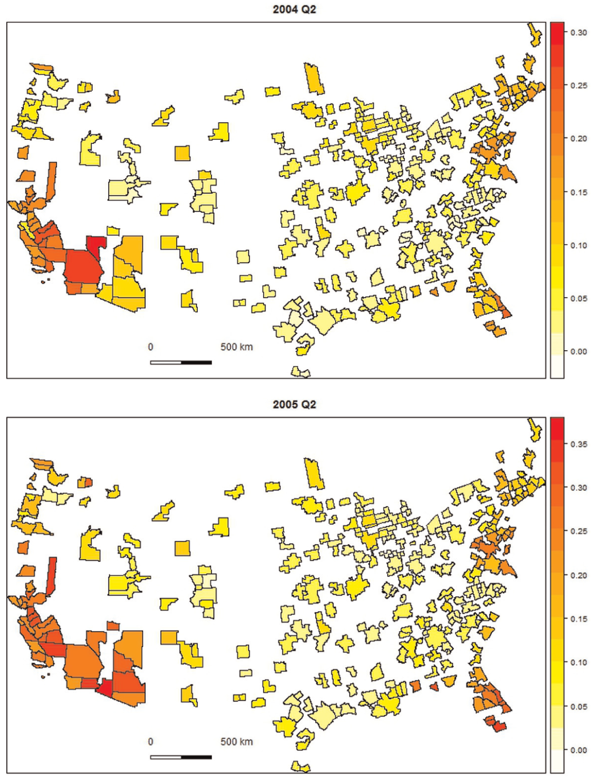
Annual growth rate of regional house prices, US metropolitan statistical areas.

Spatial dependence and spatial heterogeneity are two well established aspects of house price developments. However, differences in spatial spillovers across space and time have not yet gained much attention. A possible explanation of those differences in spillovers could be the so-called disposition effect (Shefrin and Statman, 1985). The disposition effect labels the phenomenon in financial markets that investors sell their winning stocks too soon and hold their losing stocks too long. The disposition effect also holds for the real estate market and implies a market slowdown in times of decreasing house prices. In order to avoid a nominal loss, homeowners with selling intentions set higher list prices and thereby delay selling or decide not to sell at all. This behaviour depends on the overall house price development within a certain region at a given moment in time, thus house price spillovers depending on homeowners’ behaviour will also vary across regions and time. Accordingly, the disposition effect implies reduced house price spillovers in times of declining house prices. Assuming incorrectly homogeneous spillovers across space and time could give a misleading picture of local house price dynamics.

A panel smooth transition regression model is used that allows to jointly analyse these three aspects of spatial data. González et al. (2005) develop this model in order to describe heterogeneous panels, where the coefficients can vary between regions and with time. Spatial dependence is introduced by including the spatial lag of house prices, spatial heterogeneity is introduced by allowing the fundamentals to have heterogeneous effects across time and space, and heterogeneity in house price spillovers is introduced by allowing the spatial dependence parameter to change over time and with space. To the best of our knowledge this is the first paper providing a joint analysis of all three spatial aspects, the first paper that explicitly models heterogeneity across time and space in spatial dependence, and the first paper that tries to model the disposition effect using heterogeneity in spatial spillovers.

The results reveal that house prices in neighbouring regions spill over more in times of increasing neighbouring house prices than during times of declining neighbouring house prices. This is seen as evidence for the disposition effect. Heterogeneity in the effect of the fundamentals on house price dynamics is only found for population growth and building permits, but not for real per capita disposable income and the unemployment rate. Most importantly, this analysis shows that it is not appropriate to assume uniform house price spillovers across space and time.

Theoretical aspects and empirical evidence

Spatial dependence in house prices is also known as the ripple effect. Accordingly, house prices in one region cause house price movements in neighbouring regions (Giussani and Hadjimatheou, 1991; Meen, 1999). Migration, equity transfer, information asymmetries and the spatial patterns in the fundamentals of house prices play a key role in the spatial spillovers of house prices (Meen, 1999). Migration or equity transfer to regions where house prices are comparably low could lead to the ripple effect by increasing demand and thereby prices. Information asymmetries may imply that new information regarding the housing market available in one area are transmitted only gradually to other submarkets. Finally, the ripple effect could appear if variables explaining house prices themselves show a spatial pattern.

Empirical evidence regarding spatial spillovers of house prices is quite strong. Kuethe and Pede (2011) find in their analysis of house prices in Western USA that in-state housing price forecasts can be improved by using housing prices from neighbouring states. Furthermore, their results indicate that previous house prices in space and time impact current house prices. Similarly, Holly et al. (2011) find dynamic spillover effects of house prices from the neighbouring regions. Brady (2011) analyses the dynamics of regional house prices across space and over time. Using impulse response functions, he finds that for a given shock the diffusion of regional house prices in California counties across space lasts up to two and a half years.¹

But, housing markets exhibit not only spatial dependence but also spatial heterogeneity. Following Wood (2003), one reason for spatial heterogeneity could be that some regions respond more rapidly to national economic shocks than others because their housing market is more liquid and new information is reflected more quickly in the house prices. Meen (1999) argues that heterogeneity arises because of different household behaviour and household composition. Moreover, the supply of housing could be limited by planning constraints or by geographical constraints such as mountains or lakes. Thus, house prices react differently to changes in demand conditions if supply cannot adjust.

Empirical evidence for spatial heterogeneity is found by van Dijk et al. (2011), who detect the existence of two clusters of regions in the Netherlands. Regions within the cluster have the same house price dynamics, while the dynamics are different across clusters. The different clusters can be distinguished among others by the average growth rate of house prices. Furthermore, Dieleman et al. (2000) detect three clusters in their analysis of 27 metropolitan housing markets in the USA, where the clusters where chosen based on the average median price and rent level. The authors find that house prices are geographical autocorrelated within the cluster.

Heterogeneity in house price spillovers over time is analysed by de Bandt and Malik (2010) and de Bandt et al. (2010). The authors find stronger spillovers in crises times compared to normal times.² I argue that the disposition effect (Shefrin and Statman, 1985) may serve to explain differences in spillovers across time. The disposition effect is the phenomenon in financial markets that investors sell their winning stocks too soon and hold their losing stocks too long. The disposition effect also holds for the real estate market. Case and Shiller (1988), Genesove and Mayer (2001), Anenberg (2011) and Hong et al. (2014) find that the market slows down in times of decreasing house prices. Sellers, who are confronted with losses, are likely to set higher list prices. If buyers are not willing to pay these prices, houses are on the market for a longer time. Homeowners could decrease list prices, but the authors find that they do not so but instead delay selling to avoid nominal losses. Thus, decreasing prices are associated with a lower transaction volume.

The prospect theory (Kahneman and Tversky, 1979), mental accounting (Thaler, 1999), and cognitive dissonance (Festinger, 1957) are concepts that may explain the disposition effect in the real estate market.

According to prospect theory, individuals follow an S-shaped value function. Starting from a reference point, which may be the initial price paid for a house, this function is concave downward above this reference point and concave upward below this reference point. Sellers who are confronted with a capital loss demand higher prices because their marginal utility of one additional unit of capital is higher compared with homeowners with a capital gain. Given the higher list prices, the likelihood of selling their homes is smaller for homeowners with capital loss.

The concept of mental accounting means that individuals group elements of their consumption and expenditures in mental accounts. They follow their personal rules in managing those accounts and react in different ways to the investments in the different accounts. When homeowners hold on to their losing asset, it is because in their mental account the loss is only booked when the asset is sold.

Finally, ‘cognitive dissonance is the mental conflict that people experience when they are presented with evidence that their beliefs or assumptions are wrong’ (Shiller, 1999: 1314). People experiencing cognitive dissonance try to trivialise or avoid the new information, developing explanations as to why their current beliefs or assumptions should not be revised. For the housing market this would mean that homeowners avoid the information of declining house prices or try to find explanations as to why this decline does not apply to their home.

As homeowners’ selling behaviour depends on overall house price development, house price spillovers will also. Thus, the disposition effect may serve as an explanation for heterogeneity in house price spillovers. Accordingly, when the market slows down in times of decreasing house prices, spillovers are not as strong as for increasing house prices. A reason for this phenomenon is that the mechanisms leading to the ripple effect do not work the same way in times of decreasing house prices.

Regarding spatial spillovers of house prices induced by migration, Anenberg (2011) argues that homeowners may prefer staying rather than moving in order to avoid a nominal loss when selling their property. This means that, if migration as a driving force of house price spillovers slows down because of loss aversion, spillovers should also decrease.

As mentioned, Meen (1999) explains that new information regarding the housing market is transmitted only gradually. However, in times of declining house prices, homeowners will avoid new information from neighbouring regions or find explanations as to why this new information does not apply to their property – as suggested by the concept of cognitive dissonance. Thus, they will not cut their asking price even if they learn the information about further declining house prices. This behaviour should again be reflected in smaller house price spillovers.

The disposition effect may not only explain heterogeneity in house price spillovers across time but also across space. If house prices in neighbouring regions decline, the spatial spillover is expected to be smaller compared with spillovers in regions where neighbouring house prices still increase. This implies different house price spillovers at a given moment in time because of heterogeneous house price developments across regions within the country.

Econometric approach

In the first step, I simply estimate a spatial panel fixed effects regression. This allows us to get an idea of the overall spatial spillover effect of house prices. In a second step, the panel smooth transition regression model is estimated in order to capture the heterogeneity in spatial dependence across time and space as well as the heterogeneity in the effect of the fundamentals.³

Spatial fixed effects panel estimation

Including a spatial lag of the dependent variable in our panel estimation allows us to capture the spatial spillovers of house prices of the neighbouring regions. Which regions are defined as neighbours is determined by the spatial weight matrix $W_{N}$ , of dimension $N \times N$ (Anselin et al., 2008), where $N$ is the number of regions. Each element of the weight matrix, $w_{ij}$ , determines the strength of the interaction between regions $i$ and $j$ . If there is no interaction between region $i$ and $j$ , $w_{ij}$ is equal to zero. By convention, the diagonal elements, $w_{ii}$ , are equal to zero. In our estimation the weights are equal to the inverse distance, $\frac{1}{d_{ij}}$ , where $d_{ij}$ is the distance between region $i$ and $j$ . All regions within a distance of 330 km will have a positive weight in the spatial weight matrix. This distance is the smallest possible, where all regions have at least one neighbour. Furthermore, the weights are row standardised, which means that the elements of each row sum to one. This transformation implies that $W_{N}$ is no longer symmetric. For the panel case, the cross-sectional weight matrix $W_{N}$ is stacked $T$ times. Thus, I assume that the spatial weight matrix does not change over time.

W_{NT} = I_{T} \otimes W_{N}

(1)

The vector of spatially lagged dependent variables is written as:

Wy = W_{NT} y = (I_{T} \otimes W_{N}) y .

(2)

Following Elhorst (2014), the general notation of the estimated fixed effects spatial lag model is:⁴

Y_{t} = ρ {WY}_{t - 1} + X_{t} β + μ + ξ_{t} ι_{N} + ε_{t}

(3)

where $Y_{t}$ is an $Nx 1$ vector consisting of one observation of the dependent variable for every spatial unit $(i = 1, . . ., N)$ in the sample at time $t$ . $ρ$ is the spatial dependence parameter, $μ$ the region specific fixed effects, $ξ_{t}$ are time period specific effects, $ι_{N}$ is an $Nx 1$ vector of ones, and $X_{t}$ is an $NxK$ matrix of $K$ explanatory variables. As mentioned above, regions are hit by house prices of neighbouring regions with a certain time lag. Following the Akaike information criterion, I include the spatially lagged dependent variable lagged by one period, ${WY}_{t - 1}$ .⁵ Anselin et al. (2008) call this a pure space recursive model. Pure space recursive models can simply be estimated by ordinary least squares (OLS) (Lee and Yu, 2010). Including the lagged spatial lag is in line with other spatial house price papers (see for example Kuethe and Pede, 2011, and McGreal and de La Paz, 2013).

Brady (2014) elaborates that in the literature it is not unanimous if regional house prices are stationary. Breitung (2000) panel unit root tests are used to make sure that all variables included in the model are stationary. Thus, in our spatial fixed effects panel estimation, the dependent variable, real quarterly house price growth rate, $hpi$ , is regressed on annual population growth, $population$ ; annual growth of the unemployment rate, $unemployment$ ; annual growth of real per capita disposable income, $income$ ; the log of building permits per population, $building permits$ ; the spatial lag of the dependent variable lagged by one period, $Whpi$ ; and on quarterly time dummies, $ξ_{t}$ (equation 4).⁶ Time dummies are included to capture changes in the fundamentals that hit all regions at the same time, such as, for example, changes in the federal funds rate. Furthermore, a fixed effects regression is estimated to capture all time-invariant region-specific effects, $μ_{i}$ . The different lags of the explanatory variables are chosen based on the Akaike information criterion (AIC).⁷

{hpi}_{it} = μ_{i} + α {population}_{it - 3} + β {unemployment}_{it - 2} + ζ {income}_{it - 2} + δ building {permits}_{it - 1} + ρ \sum_{j = 1}^{N} w_{ij} {hpi}_{jt - 1} + ξ_{t} + ε_{it} .

(4)

The results of this estimation give an idea of the overall spatial dependence in house price dynamics and of the effect of the fundamentals, disregarding any heterogeneity across space or time.

Fixed effects panel smooth transition regression model

To include heterogeneity in the model, a non-dynamic fixed effects panel smooth transition regression model (PSTR) is estimated (González et al., 2005). This model allows the coefficients of the explanatory variables to vary between regions and with time. The coefficients change smoothly as a function of the transition variable and are, thereby, a continuous function of this transition variable. This model appears to be especially appropriate for our setting, as it allows the spatial dependence coefficient and the coefficients of the fundamentals to vary across space and time. Thereby, spatial heterogeneity in house prices is modelled by the changing coefficients of the fundamentals; heterogeneity in house price spillovers is modelled by the changing spatial dependence coefficient. Following González et al. (2005), the PSTR model is written as follows:

y_{it} = μ_{i} + θ'_{0} x_{it} + θ'_{1} x_{it} g (q_{it}; γ, c) + ε_{it},

(5)

where $g (q_{it}; γ, c)$ is the transition function, which is normalised to be bounded between 0 and 1. When the transition function is equal to 0, the coefficient of a given explanatory variable is $θ_{0}$ ; when the transition function is equal to 1, the coefficient is $θ_{0} + θ_{1}$ . The transition variable is $q_{it}$ . González et al. (2005) develop the PSTR model for the logistic specification of the transition function. For the case of two extreme regimes, the logistic transition function is given by:

g (q_{it}; γ, c) = \frac{1}{1 + e^{- γ (q_{it} - c)}},

(6)

where $c$ is the location parameter, and $γ$ is the slope of the transition function that determines the smoothness of the transition between two regimes. The higher $γ$ , the faster is the transition between two regimes. For $γ$ going to infinity, the transition is instantaneous. For $γ$ going to 0, the transition function becomes constant and this implies that there are no regimes at all. If the transition variable, $q_{it}$ , is smaller than the location parameter, $c$ , the transition function, $g (q_{it}; γ, c)$ , tends to 0, and the coefficients tend to $θ_{0}$ . If the transition variable, $q_{it}$ , is larger than the location parameter, $c$ , the transition function, $g (q_{it}; γ, c)$ , tends to 1, and the coefficients tend to $θ_{0} + θ_{1}$ .

In the empirical application, the transition variable should capture the source of the parameter heterogeneity. A good candidate for the transition variable in our analysis is the spatially weighted annual house price development of the neighbouring regions, ${Whpiag}_{t - 1}$ . There are several reasons for this choice: First, de Bandt and Malik (2010) and de Bandt et al. (2010) find stronger spillovers in crises times when compared with normal times. Normal times in the housing market could be expressed by relatively normal average house price developments, while crisis times would be expressed by extreme increases or decreases in housing prices. Taking spatially weighted neighbouring house prices should be a good approximation for the overall house price development in the larger geographical region where an MSA is located.

Second, this variable seems to be a good candidate for the transition variable, as Dieleman et al. (2000) and van Dijk et al. (2011) find different house price developments within clusters, where the clusters are defined by average house price growth rates. Again, neighbouring house prices should be a good approximation of the average house price development in the larger geographical region where an MSA is located.

Third, the disposition effect for the housing market implies that homeowners do not react as strongly to signals of declining house prices as to signals of increasing house prices. It is reasonable to assume that those signals come from neighbouring regions. Therefore, the transition variable formed by the spatially weighted house prices of the neighbouring regions should be able to model the disposition effect in the housing market. In this respect, the logistic specification of the PSTR model, compared with an exponential specification, is appropriate for this setting as I expect different spillovers depending on whether one is above or below the location parameter, $c$ . This consideration together with the fact that the estimation is conducted over a relative short time span of 21 quarters, it is reasonable to assume that there are only two extreme regimes.

In sum, the transition variable allows us to capture heterogeneity in spatial house price spillovers and heterogeneity in the effect of the fundamentals on house prices. However, I am aware that this transition variable does not capture heterogeneity in spatial spillovers because of different migration patterns or different amounts of information asymmetries.⁸

The PSTR model for our estimation of US regional house price dynamics is written as:

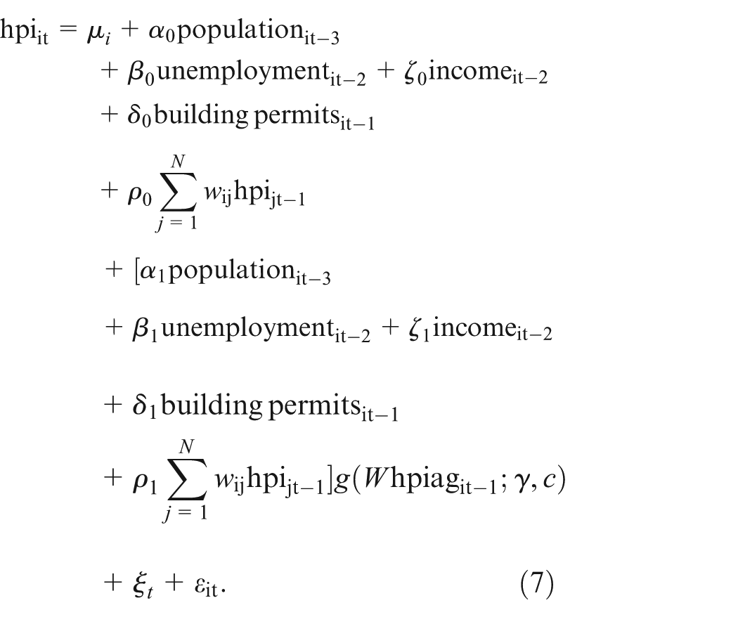
{hpi}_{it} = μ_{i} + α_{0} {population}_{it - 3} + β_{0} {unemployment}_{it - 2} + ζ_{0} {income}_{it - 2} + δ_{0} {buildingpermits}_{it - 1} + ρ_{0} \sum_{j = 1}^{N} w_{ij} {hpi}_{jt - 1} + [α_{1} {population}_{it - 3} + β_{1} {unemployment}_{it - 2} + ζ_{1} {income}_{it - 2} + δ_{1} building {permits}_{it - 1} + ρ_{1} \sum_{j = 1}^{N} w_{ij} {hpi}_{jt - 1}] g (W {hpiag}_{it - 1}; γ, c) + ξ_{t} + ε_{it} .

(7)

Later the notation $Θ_{p} = (α_{p} β_{p} ζ_{p} δ_{p} ρ_{p})$ for $p = (0, 1)$ is used. If two extreme regimes are assumed, the transition function, $g (W {hpiag}_{it - 1}; γ, c)$ , will tend to 1 for high values of the transition variable, $W {hpiag}_{it - 1}$ . This implies that whenever one observes high neighbouring house price growth rates, the spatial spillover parameter will tend to $ρ_{0} + ρ_{1}$ and, correspondingly the other explanatory variables. Whenever one observes low or decreasing neighbouring house price growth rates, the spatial spillover parameter will tend to $ρ_{0}$ , and, correspondingly the other explanatory variables. In the estimation $ρ_{0}$ is expected to be smaller than $ρ_{0} + ρ_{1}$ , as the disposition effect predicts smaller house price spillovers in times of declining house prices.⁹

Data description

Data for 319 metropolitan statistical areas are used. Out of the existing 366 MSAs in 2012, I chose this sample because of data availability issues. Figure 3 plots the 319 MSAs used in the estimation. Following the United States Census Bureau, ‘the general concept of a metropolitan area is that of a large population nucleus, together with adjacent communities having a high degree of social and economic integration with that core’ (Federal Register, 2010: 37,246).

For the dependent variable, house prices, the Federal Housing Finance Agency all-transactions quarterly index is used. Furthermore, data on annual nominal per capita disposable income and population come from the Bureau of Economic Analysis. Annual population data are transferred to quarterly data using linear interpolation. Annual per capita disposable income is transferred to quarterly data using cubic spline. Applying cubic spline has the advantage that the resulting data are smooth in the first derivative. In order to get real values of house prices and per capita disposable income, the nominal values are divided by the consumer price index. Using real variables is in line with the literature on house price dynamics. However, this will not allow us to exactly compare our results with Genesove and Mayer (2001) and Engelhardt (2003), who find that loss aversion in the housing market depends on nominal loss. The regional annual consumer price index (all urban consumers) is obtained from the Bureau of Labor Statistics. The index is available for 27 larger geographical areas. Again, quarterly data are obtained by using cubic spline. Monthly unemployment rates from the Bureau of Labor Statistics are transferred to quarterly data by taking the quarterly averages. Population density is calculated using the population data mentioned above and the land area taken from the TIGER/Line shapefiles from the United States Census Bureau. Monthly new privately owned housing units authorised are taken from the United States Census Bureau.¹⁰ Quarterly data are obtained by using the sum of the monthly building permits. Building permits are divided by population. Unfortunately data for the effective mortgage interest rate are not available for all 319 MSAs (Mikhed and Zemcík, 2009). However, I include time dummies to capture changes in the fundamentals that hit all regions at the same time, such as for example changes in the federal funds rate.

Empirical results

To get an idea of the overall spatial dependence, disregarding any heterogeneity across space or time, I start with the spatial fixed effects panel estimation, where real quarterly house price growth rates are regressed on annual population growth, annual growth of the unemployment rate, annual growth of real per capita disposable income, the log of building permits per population, the spatial lag of the dependent variable, and on quarterly time dummies. Because data on building permits are only available over a rather short time span, the estimation is conducted for the period 2004Q2 to 2009Q2 (Table 1). Over this time span a balanced panel is available for 319 regions. The standard errors presented are Huber–White heteroscedasticity consistent (Huber, 1967; White, 1980). Those standard errors allow for not just heteroscedasticity in the standard errors but also for autocorrelation among observations within one cluster, where clustering takes place by MSA.

Table 1.

Spatial panel estimation.

Dependent variable: quarterly real house price growth rate, hpi
Variable	FE (Fixed effects) coefficients	Huber–White standard errors
α population_t-3	0.26***	0.10
β unemployment_t-2	−0.003	0.003
ζ income_t-2	0.14***	0.02
δ building permits_t-1	0.003***	0.0007
ρ W × hpi_t-1	0.73***	0.04
R ²	0.61
AIC	−8.3692
Observations	6699
Number of groups	319
Time period	2004Q2–2009Q2
Time dummies	yes

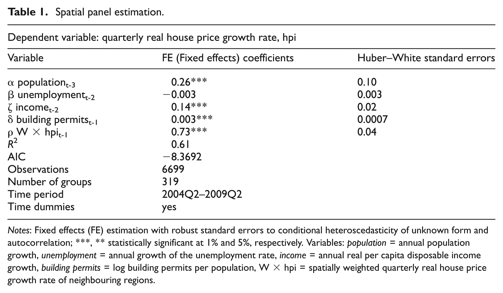
Notes: Fixed effects (FE) estimation with robust standard errors to conditional heteroscedasticity of unknown form and autocorrelation; ***, ** statistically significant at 1% and 5%, respectively. Variables: population = annual population growth, unemployment = annual growth of the unemployment rate, income = annual real per capita disposable income growth, building permits = log building permits per population, W × hpi = spatially weighted quarterly real house price growth rate of neighbouring regions.

With this spatial panel estimation I want to capture the spatial spillovers in house prices, however, I cannot make the distinction between spatial spillover and common shocks that hit some MSAs instantaneously and some with a time lag.¹¹ It could be that a common shock hits first some regions with a very liquid housing market and reaches others with a certain time delay. The estimation would mistake this different timing in the reaction to a common shock as spillover of house prices. As I cannot differentiate between common shocks with region specific reaction time and spatial spillovers, the coefficient of the spatially lagged dependent variable is probably overestimated.

The results point to a strong spillover effect of neighbouring house prices. Furthermore, the estimation results reveal a positive effect of population and real per capita disposable income growth on house price growth rates. An expected negative effect of increasing unemployment rates on house price growth rates turns out not to be significant. Building permits are associated with higher house price growth rates. This implies that building permits primarily mirror increased demand for housing and not increased supply where house prices would be expected to fall. However, the coefficients assume the same strength of the spatial spillover or the same effect of the fundamentals no matter which region or time period one is looking at. These global effects could be misleading locally. The panel smooth transition regression model will help determine whether these coefficients hold for all regions in every single time period.

The results of the panel smooth transition regression in the case of two extreme regimes are presented in Table 2, the corresponding transition function is plotted in Figure 2.¹² For almost all negative values of the transition variable, i.e. decreasing neighbouring house prices, the transition function is equal to 0. This implies that the coefficients of the different explanatory variables are equal to $Θ_{0}$ in case of decreasing neighbouring house prices, where $Θ_{0} = (α_{0} β_{0} ζ_{0} δ_{0} ρ_{0})$ . Furthermore, the transition function is equal to 1 for very high growth rates of neighbouring house prices of above 15%. For those high growth rates of neighbouring house prices, the coefficients of the explanatory variables are equal to $Θ_{0} + Θ_{1}$ . The location parameter, $c$ , is equal to 0.07, which implies that when neighbouring house prices grow, on average, by 7%, the coefficient is equal to $Θ_{0} + 0.5 \times Θ_{1}$ . The slope parameter, $γ$ , is equal to 37.49. In the literature such a value is not assumed to imply an instantaneous transition between regimes but a relatively smooth transition (Lee and Chien, 2011; Trupkin and Ibarra, 2011).

Table 2.

PSTR estimation results, two extreme regimes.

Dependent variable: quarterly real house price growth rate, hpi
Variable	Coefficients	Huber–White t-statistic	Difference between coefficients
α₀ population_t-3	0.07	1.43
β₀ unemployment_t-2	−0.02***	−11.34
ζ₀ income_t-2	0.13***	7.46
δ₀ building permits_t-1	0.005***	9.41
ρ₀ W × hpi_t-1	0.33***	9.39
α₀+α₁ population_t-3	0.50***	8.60	−5.73***
β₀+β₁ unemployment_t-2	0.05***	9.95	−11.41***
ζ₀+ζ₁ income_t-2	0.18***	5.36	−1.40
δ₀+δ₁ building permits_t-1	0.002***	3.76	3.97***
ρ₀+ρ₁ W × hpi_t-1	0.60***	17.37	−5.44***
γ, slope	37.49
c, location parameter	0.07
R ²	0.63
AIC	−8.3949
Observations	6699
Number of groups	319
Time period	2004Q2–2009Q2
Time dummies	yes

Notes: Fixed effects estimation with robust standard errors to conditional heteroscedasticity of unknown form; ***, ** statistically significant at 1% and 5%, respectively. Variables: population = annual population growth, unemployment = annual growth of the unemployment rate, income = annual real per capita disposable income growth, building permits = log building permits per population, W × hpi = spatially weighted quarterly real house price growth rate of neighbouring regions.

Figure 2.

Transition function versus transition variable, two extreme regimes.

Most interestingly, the coefficient of the spatially lagged dependent variable is much smaller in case of decreasing neighbouring house prices, $ρ_{0} = 0.33$ , than in case of strongly increasing neighbouring house prices, $ρ_{0} + ρ_{1} = 0.6$ . That means that house prices in neighbouring regions spill over more in times of increasing neighbouring house prices than during times of declining neighbouring house prices. This is interpreted as evidence for the disposition effect. Because of loss aversion, homeowners delay selling or abandon their selling intention in times of decreasing house prices. They will not adjust list prices downward even if they learn new information about declining house prices in neighbouring regions and even if doing so would increase the likelihood of selling their property. Thus, the theory that house prices spill over because of information asymmetries no longer holds in times of decreasing house prices. The same is true for transmission through migration. Homeowners with moving intentions are likely not to sell at all their property because they are not willing to adjust prices downward. So moving is delayed or abandoned. If transactions are not operated, as predicted by the disposition effect, house prices simply do not spill over as strongly as in times of increasing house prices. Thus, our results confirm the findings by Genesove and Mayer (2001), Engelhardt (2003), Anenberg (2011), and Hong et al. (2014) of loss aversion. However, the authors analyse nominal and not real loss aversion as I do.

Overall, I find evidence for heterogeneity in spatial spillovers of house prices across space and time. This confirms and augments the findings by Gray (2012) of heterogeneity in house price spillovers across space.

Figure 3 is a plot of the individual coefficients of the spatially lagged dependent variable for four points in time and reveals the amount of heterogeneity across time and space in spatial house price spillovers. The plotted coefficients vary between $ρ_{0} = 0.33$ , implying weak spatial spillovers of house prices, and $ρ_{0} + ρ_{1} = 0.60$ , implying strong spatial spillovers of house prices. Those strong spillovers are especially observed for the coastal regions for example in 2004Q2, or 2005Q3. The house price spillovers in the inland at that time are more at the lower bound of 0.33. When house prices started to decline at the end of 2006, the spillovers quickly declined in the coastal regions and reached the lower bound of 0.33 in 2008Q1 in almost all regions. Moreover, 4192 out of 6699 observations overall (319 regions over 21 time periods) have coefficients between 0.4 and 0.5, as compared with the extreme regime coefficients $ρ_{0}$ =0.33 and $ρ_{0} + ρ_{1} = 0.6$ . Thus, assuming only two extreme regimes without smooth transition between them would not be appropriate for more than 60% of all observations.

Figure 3.

Individual spatial spillover parameters at different points in time, two extreme regimes.

The estimation results further indicate that there is no heterogeneity in the effect of real per capita disposable income on house prices, as the test statistic reveals no significant difference between the coefficients $ζ_{0}$ and $ζ_{0} + ζ_{1}$ . The coefficient on the unemployment rate is significantly negative in one extreme regime and significantly positive in the other extreme regime. The coefficients between $β_{0}$ and $β_{0} + β_{1}$ are close to zero and probably insignificant, as in the spatial panel regressions. Therefore one should not worry about the unreasonable positive effect of the unemployment rate in times of very high house price growth rates. Moreover, the coefficient of population growth is insignificant in times of decreasing neighbouring house prices and becomes significant when neighbouring house prices increase. This result implies that, compared with the strong increases, the strong decline in house prices in the sample period could less be explained by population growth. However, the development of building permits, reflecting demand for housing, have a larger effect on house prices in times of decreasing neighbouring house prices. As the detected heterogeneity in the effects of population growth and building permits on house prices point in opposite directions, one cannot conclude that fundamentals serve more or less to explain house prices in times of decreasing or increasing neighbouring house prices. In sum, heterogeneity in the effect of the fundamentals on house price dynamics could not be detected for all variables; real per capita disposable income and the unemployment rate have a homogeneous effect across time and space.

The test of no remaining non-linearity proposed by González et al. (2005) confirms that the linear model presented in Table 1 is not appropriate. Furthermore, the $R^{2}$ and the AIC confirm an improvement of the non-linear model over the linear model.

Conclusion

This paper is a joint analysis of three spatial characteristics in house price dynamics, namely spatial dependence, spatial heterogeneity and heterogeneity in spatial dependence. While spatial dependence and spatial heterogeneity are well established aspects of house price developments, heterogeneity in spatial dependence has not gained much attention yet. I argue that the disposition effect may explain different house price spillovers across space and time. Assuming incorrectly homogeneous spillovers could locally give a misleading picture of house price dynamics.

First, a spatial panel regression is estimated to see whether there is overall spatial dependence in house price developments. Subsequently, a panel smooth transition regression model is applied to estimate the heterogeneity across space and time in spatial dependence and in the effect of the fundamentals on house price dynamics.

The results reveal strong house price spillovers when the average annual house price increase of the neighbouring regions is greater than 15%. Significant lower house price spillovers are detected for times of declining house prices in the neighbouring regions. This is seen as evidence for the disposition effect. Because of loss aversion, homeowners with selling intentions will not adjust prices downward, even if they get signals of declining house prices in neighbouring regions. This behaviour reduces the transaction volume in the housing market and, consequently reduces house price spillovers. Our results confirm previous findings by Genesove and Mayer (2001), Engelhardt (2003), Anenberg (2011) and Hong et al. (2014) of loss aversion in the housing market.

Heterogeneity in the effect of the fundamentals on house price dynamics is only found for population growth and building permits, but not for real per capita disposable income and the unemployment rate.

This analysis shows that it is not appropriate to assume uniform house price spillovers across space and time. In times of declining house prices the spillovers are much lower than what linear estimations suggest. The panel smooth transition regression model is an appropriate tool to model those non-linearities in spatial spillovers across time and space.

Footnotes

Funding

This research received no specific grant from any funding agency in the public, commercial, or not-for-profit sectors.

Notes

References

Anenberg

(2011) Loss aversion, equity constraints and seller behavior in the real estate market. Regional Science and Urban Economics 41(1): 67–76.

Anselin

(1988) Spatial Econometrics: Methods and Models. Dodrecht, The Netherlands: Kluwer Academic Publishers.

Anselin

Gallo

Jayet

(2008) Spatial panel econometrics. In: Mátyás

Sevestre

(eds) The Econometrics of Panel Data. Advanced Studies in Theoretical and Applied Econometrics, Volume 46. Berlin, Heidelberg: Springer, pp. 625–660.

Brady

(2011) Measuring the diﬀusion of housing prices across space and over time. Journal of Applied Econometrics 26(2): 213–231.

Brady

(2014) The spatial diﬀusion of regional housing prices across US states. Regional Science and Urban Economics 46: 150–166.

Breitung

(2000) The local power of some unit root tests for panel data. In: Advances in Econometrics, Vol. 15: Nonstationary Panels, Panel Cointegration, and Dynamic Panel. New York: Elsevier, JAI Press, pp. 161–178.

Case

Shiller

(1988) The behavior of home buyers in boom and post-boom markets. New England Economic ReviewNov: 29–46.

de Bandt

Malik

(2010) Is there evidence of shift-contagion in international housing markets?Banque de France Working Paper295, Banque de France.

de Bandt

Barhoumi

Bruneau

(2010) The international transmission of house price shocks. In: de Bandt

Knetsch

Penalosa

. (eds) Housing Markets in Europe. Berlin, Heidelberg: Springer, pp. 129–158.

10.

Debarsy

Ertur

LeSage

(2012) Interpreting dynamic space-time panel data models. Statistical Methodology 9(1): 158–171.

11.

Dieleman

Clark

WAV

Deurloo

(2000) The geography of residential turnover in twenty-seven large US metropolitan housing markets, 1985–95. Urban Studies 37(2): 223–245.

12.

Elhorst

(2014) Spatial Econometrics: From Cross-sectional Data to Spatial Panels. Berlin, Heidelberg: Springer.

13.

Engelhardt

(2003) Nominal loss aversion, housing equity constraints, and household mobility: Evidence from the United States. Journal of Urban Economics 53(1): 171–195.

14.

Federal Register (2010) 2010 Standards for delineating metropolitan and micropolitan statistical areas. Federal Register 75(123): 37,246–37,252.

15.

Festinger

(1957) A Theory of Cognitive Dissonance. Redwood City, CA: Stanford University Press.

16.

Genesove

Mayer

(2001) Loss aversion and seller behavior: Evidence from the housing market. The Quarterly Journal of Economics 116(4): 1233–1260.

17.

Giussani

Hadjimatheou

(1991) Modeling regional house prices in the United Kingdom. Papers in Regional Science 70(2): 201–219.

18.

González

Teräsvirta

van Dijk

(2005) Panel smooth transition regression models. Working Paper Series in Economics and Finance604, Stockholm School of Economics.

19.

Gray

(2012) District house price movements in England and Wales 1997–2007: An exploratory spatial data analysis approach. Urban Studies 49(7): 1411–1434.

20.

Holly

Pesaran

Yamagata

(2011) The spatial and temporal diﬀusion of house prices in the UK. Journal of Urban Economics 69(1): 2–23.

21.

Hong

Loh

Warachka

(2014) The impact of gains and losses on homeowner decisions. Technical report. Available at: http://papers.ssrn.com/sol3/papers.cfm?abstract_id=2509599.

22.

Huber

(1967) The behavior of maximum likelihood estimates under nonstandard conditions. In: Lecam

Neyman

(eds) Proceedings of the 5th Berkeley Symposium on Mathematical Statistics and Probability. Berkeley and Los Angeles: University of California Press. Volume 1(1), pp. 221–233.

23.

Kahneman

Tversky

(1979) Prospect theory: An analysis of decision under risk. Econometrica 47(2): 263–291.

24.

Kodres

Pritsker

(2002) A rational expectations model of financial contagion. The Journal of Finance 57(2): 769–799.

25.

Kuethe

Pede

(2011) Regional housing price cycles: A spatio-temporal analysis using US state-level data. Regional Studies 45(5): 563–574.

26.

Lee

C-C

Chien

M-S

(2011) Empirical modelling of regional house prices and the ripple eﬀect. Urban Studies 48(10): 2029–2047.

27.

Lee

L-f

(2010) Some recent developments in spatial panel data models. Regional Science and Urban Economics 40(5): 255–271.

28.

LeSage

Pace

(2009) Introduction to Spatial Econometrics. Boca Raton: Chapman & Hall/CRC.

29.

McGreal

de La Paz

(2013) Implicit house prices: Variation over time and space in Spain. Urban Studies 50(10): 2024–2043.

30.

Meen

(1999) Regional house prices and the ripple eﬀect: A new interpretation. Housing Studies 14(6): 733–753.

31.

Mikhed

Zemcík

(2009) Do house prices reflect fundamentals? Aggregate and panel data evidence. Journal of Housing Economics 18(2): 140–149.

32.

Molloy

Smith

Wozniak

(2011) Internal migration in the United States. NBER Working Paper17307, National Bureau of Economic Research.

33.

Shefrin

Statman

(1985) The disposition to sell winners too early and ride losers too long: Theory and evidence. The Journal of Finance 40(3): 777–790.

34.

Shiller

(1999) Human behavior and the eﬃciency of the financial system. In: Taylor

Woodford

(eds) Handbook of Macroeconomics. Volume 1. Amsterdam: Elsevier, Chapter 20, pp. 1305–1340.

35.

Teräsvirta

(1994) Specification, estimation, and evaluation of smooth transition autoregressive models. Journal of the American Statistical Association 89(425): 208–218.

36.

Thaler

(1999) Mental accounting matters. Journal of Behavioral Decision Making 12(3): 183–206.

37.

Trupkin

Ibarra

(2011) The relationship between inflation and growth: A panel smooth transition regression approach for developed and developing countries. Documentos de Trabajo/Working Papers1107, Facultad de Ciencias Empresariales y Economia. Universidad de Montevideo.

38.

van Dijk

Franses

Paap

. (2011) Modelling regional house prices. Applied Economics 43(17): 2097–2110.

39.

White

(1980) A heteroskedasticity-consistent covariance matrix estimator and a direct test for heteroskedasticity. Econometrica 48(4): 817–838.

40.

Wood

(2003) The information content of regional house prices: Can they be used to improve national house price forecasts?Bank of England Quarterly Bulletin, Autumn, 304–314.