Distance to work in Beijing: Institutional reform and bargaining power

Abstract

In this study, we use a large sample from the Beijing Household Travel Survey to build husband-wife dyads, construct variables to measure bargaining power between spouses and place intra-household travel arrangements within a broader institutional framework to analyse relationships between institutions, bargaining power and travel patterns of married men and women. The empirical results reveal that bargaining power does matter in determining intra-household commute arrangements. The overarching institutional framework meanwhile sets boundaries for bargaining, and defines which resources are effective bargaining chips for individuals.

Keywords

bargaining power Beijing distance to work gender institutional reform

Introduction

In the ordinary course of their lives, people make many choices that affect the opportunities they will face in the future. Earning a degree, starting or dissolving a family, rearing a child, accepting or rejecting a job offer, buying a residential property, retiring from a career position – each of these decisions will affect the resources and opportunities from which individuals derive utility and sustain their lives (Lundberg and Pollak, 2003).

Economists have used basic economic tools, such as the utility maximisation framework, to explain these individual choices. The basic premise underlying this framework assumes that individuals make choices to maximise their well-being, subject to resource constraints. As the household is one of the basic decision units in society, this traditional utility maximisation framework has been applied at the household level, and has in fact been dominant in mainstream economics for a long time in analysing household choices.

In this rational unitary model of the household, the household is treated as an undifferentiated unit governed by an altruistic (in terms of their household) household head. Household members are assumed to pool their resources to maximise a neoclassical household utility function on the basis of a set of common preferences and a common budget constraint (Agarwal, 1997). As Becker (1981) puts it: ‘in my approach, the “optimal reallocation” results from altruism and voluntary contributions, and the “group function” is identical to that of the altruistic head, even when he does not have sovereign power (p. 192)’ (quoted in Sen, 1987: 15) Essentially, as long as the household remains intact, it is treated by the rational unitary model ‘as if it acts as a single individual’ (Thomas, 1990: 636). The traditional model of location and land use developed by Alonso (1964) belongs to this rational unitary model of the household.

While the application of utility maximisation gives us a very powerful tool for creating tractable economic models, it has been well recognised that the household is actually constituted of multiple members who may have different, sometimes conflicting, preferences and interests, and may have different abilities to pursue their interests (Agarwal, 1997). There are incentives for household members to be altruistic and work together for the common good. But there are also incentives for them not to pool resources but rather to ‘allocate resources over which they have discretion toward goods they especially care about’ (Thomas, 1990: 636). Thus, extensive conflicts and pervasive cooperation are both presented in household arrangements (Sen, 1987). Household arrangements regarding ‘who does what, who gets to consume what, and who takes what decisions’ can be seen as responses to the relative bargaining power of individual household members through control of resources inside and outside the household (Agarwal, 1997; Lundberg and Pollak, 2003; Sen, 1987: 13). Meanwhile, any choice made by the household may yield a different level of utility for each household member, and may affect their bargaining power and subsequent outcomes of bargaining at a later point in time.

In this paper, we take work trip distance as one of the outcomes from the choices made by household members to analyse intra-household commute arrangements. It is well recognised that individual utility is affected by work trip distances because commuting is costly in both money and time. Thus, where a household resides and how much commute distance can be accepted by household members may not be immune from the intra-household bargaining process. When a couple decides where they live and work, the pair may consider both utility of the whole household and individual outcomes. Locational decisions and thus resulting commute distances are likely subject to an explicit or implicit negotiation process, through which household members try to satisfy their own interests.

One inevitable dimension of work trip arrangements at household level is represented by gender difference in journey-to-work. As female labour force participation and multiple-earner households grew quickly in the last several decades, this gender difference in commuting has been extensively studied. There is a body of empirical studies comparing commuting patterns between men and women. The consistent findings suggest that employed women tend to have shorter commutes to work than employed men both in time and distance (Blumen, 1994; Hanson and Johnston, 1985; Hanson and Pratt, 1990; McLafferty and Preston, 1991; Madden, 1981; Turner and Niemeier, 1997). This gender difference may be due to different labour characteristics and household commitments for men and women. On average, women earn less, have higher probabilities of working in female-dominated jobs and have greater household and childcare responsibilities (Blumen, 1994; Brun and Fagnani, 1994; Hanson and Hanson, 1980; Hanson and Johnston, 1985; Johnston-Anumonwo, 1992; Madden, 1981; Michelson, 1988; Pinch and Storey, 1992; Pratt and Hanson, 1991; Robinson, 1988; Shelton and Daphne, 1993; Turner and Niemeier, 1997). Female-dominated jobs are typically more evenly distributed geographically across urban areas than male-dominated jobs, which contributes to shorter commutes for women (Hanson and Johnston, 1985). Demanding domestic duties impose greater time constraints on women, making employed women more likely to choose shorter commutes than employed men.

However, almost all of the studies referred to in this paper combined female and male observations to investigate gender differences in commuting patterns. The data in these studies generally incorporate marital status for each individual, but do not have enough information to identify specific couples. Although this approach in existing literature can consistently model average commuting patterns for men and women, it lacks information essential to diagnose the strategic dimension of joint decision-making processes within couples. Bargaining power between spouses is thus ignored in the existing literature.

In this paper, we propose to use a bargaining model to analyse: 1) how intra-household gender asymmetries in commute distance are constructed; 2) what factors affect bargaining power between couples; and 3) what the magnitude of these effects is. We anticipate that this approach can explicitly take into account specific coordination problems that arise between marriage partners and can shed light on intra-household arrangements regarding commuting patterns in an urban area in China (Abraham and Nisic, 2012).

This bargaining model could however go awry if intra-household arrangements are assumed to exist in total isolation (Agarwal, 1997). Households are embedded in socio-economic and legal institutions. Bargaining power structure within the household is to some extent preconditioned on the extra-household institutional framework, which includes community rules, social norms and legal systems. These institutions set limits to bargaining and ‘define which issues can legitimately be bargained over, and which fall in the arena of the uncontestable’ (Agarwal, 1997: 15). The function of macro-level institutions, however, is inadequately examined in the existing literature. Part of the reason is that the majority of the existing literature focused their subjects in the United States, Canada or European countries, where market forces play a very important role in shaping individual incentives. By contrast, China has undergone a major shift from command-and-control planning toward a more market-oriented system in provision of housing and jobs over the last four decades. This institutional reform in China sets up a potentially ideal platform to investigate the relationship between macro-level institutions and the job-housing spatial relationship for couples. This is also the third research question covered in this paper.

The remainder of the paper is organised as follows. The next section provides an overview of gender role and market reform in China. We then present the empirical framework. This is followed by a discussion of the data and the empirical results. The final section concludes the paper.

Gender role and market reform in China

In China, the evolution of women’s employment, education and family roles was set in motion through the political, social and economic upheaval of the revolution in 1950s (Wolf, 1985: 1). Before 1949, women in China had been largely governed by a patriarchal regime of male domination for at least 22 centuries. They were defined by male ideology, and could be cared for or disposed of by males as they saw fit. Girls were universally denied education. Their worth in traditional Chinese families was deeply ‘tied to their reproductive and caretaking roles’ (Robinson, 1985: 34).

After 1949, the Chinese Communist Party undertook various initiatives to relieve women from their past oppression. In 1950, The Marriage Law was passed to prohibit concubinage, support monogamous marriage, and to give women ‘the right to marry a person of their own choice, and the right to divorce’ (Rai, 1994: 408). Land reform in the early 1950s allowed deeds to be made out in women’s names, and gave women a right to share in family inheritances (Rai, 1994; Wolf, 1985). Education for women and their rights to enter the paid labour force were institutionalised for the first time in China (Rai, 1994). With these initiatives, women’s labour force participation and literacy rate increased substantially over a decade after 1949. A real difference was indeed made to the lives of hundreds of millions of women in China (Rai, 1994).

Yet the increase in female labour force participation and literacy should not be taken to be equivalent to full equalisation of status between men and women in the public and private spheres in China (Robinson, 1985). Family ‘was not challenged as a site of women’s oppression but only modified to embody “proletarian value”’ (Rai, 1994: 411). Women continued to be placed in a subordinate position, both at home and work. Paternalistic ‘protection’ was still ubiquitous in women’s daily life in urban China.

Let’s take housing distribution as an example. Before economic reform in 1980s, socialist housing policies prior to economic reform virtually eliminated the former private housing market in China, leaving the state as the ‘only one source of housing investment in Chinese cities’ (Wang and Murie, 1996: 982). Work units or municipal housing bureaus became effective monopolies in supplying state-funded housing to urban residents. Without work units or state organisations, there was very little chance for urban residents to find a job or a place to live in urban China.¹

In this socialist regime, occupational ranks and seniority levels in the work units or state organisations, rather than financial capabilities, became very important criteria to distribute housing properties to urban households. The higher one’s status and seniority level, the better chance one had to get housing space, or a larger housing space. Due to the shortage of housing properties in urban China, two-earner couples in two different work units could only hope to get living space from one of their work units. Yet, by tradition, women in China were expected to ‘marry up’ and follow the norm of virilocal residence (this tradition hasn’t changed much even today in 2015). Thus, the residence for a couple was more likely to be provided by the husband’s work unit (Wang, 2011; Zhuo, 1999). With this housing distribution pattern in old regime, husbands could be more likely to live close to their work places than were their wives.

Since 1978, the shift from central planning toward a market-based economy in China restructured the distribution of jobs and housing properties. As market competition and exchange became more entrenched, direct control by work units or state institutions of housing provision and job assignment was gradually relinquished and finally abolished in urban China at the end of 1990s. In 1998, the central government of China issued A Notification from the State Council on Further Deepening the Reform of the Urban Housing System and Accelerating Housing Construction. This policy specifically prohibited work units from buying or building new housing properties for employees (Deng et al., 2011). It also urged local governments to end internal allocation of existing housing properties to employees at discounted or subsidised prices (Yu, 2011: 121). By then, China ‘completed the revolutionary transition from a state-sponsored welfare housing provision system to an open commercial housing market’ in urban areas (Chen et al., 2011: 2). In 1997, China also officially abolished the centralised job assignment policy for college graduates. From then on, graduates officially had both the freedom and burden of finding their own positions and selecting from job offers.

After these sweeping reforms, Chinese citizens in cities were no longer dependent on state-owned or collective enterprises as the only places to find jobs or homes. For women in China, markets and freedom from state mandates are a mixed blessing. On the one hand, the market is associated with insecurity and lack of state protection. On the other hand, it represents mobility and freedom to choose. Women in China have increased their investments in formal education. Their earnings have risen and their ‘occupations [have] changed from more traditional ones to those that had been considered non-traditional’ (Goldin, 2006: 19). Contemporary Chinese women have larger plans for their careers than did previous generations, and they are generally influenced less than before by their husbands’ earnings (Goldin, 2006). Women in China are no longer purely subordinate actors in their families or the society. They have begun to find their own individualities and identities in jobs and professions as well as in families, which in turn is re-shaping the nature of bargaining power between spouses and influencing various choices including those about job and housing location.

Empirical framework

In this paper, we use two model specifications to investigate our research questions. The first model specification is proposed to empirically analyse general gender differences in work trip distance. Because work trip distance values are all positive, the distribution of the dependent variable is no longer normal. We then use the generalised linear regression model (GLM) to construct the first model specification as:

\begin{matrix} g {E (y 1)} & = α * Gender \\ + T β + K γ + μ, y ~ F \end{matrix}

(1)

where, g() is the link function and F is the distributional family. The Box-Cox regression and modified Park test are used to define link function and variant structure, which are log link function and gamma distributions of variant structure, respectively (Manning and Mullahy, 2001; Manning et al., 2005). y1 stands for work trip distance. T is a matrix of institutional indicators. ‘Gender’ and T are the key explanatory variables in this model specification. K represents a set of control variables, which include indicators for individual characteristics other than gender, household characteristics and spatial characteristics related to residential and work locations.

To investigate whether, and to what extent, bargaining power between the members of a couple shapes job-housing spatial relationships, and how institutions play a role in this relationship, we propose a second model specification, formulated as:

y 2 = f (X, R, Z)

(2)

where, the job-housing spatial relationship between members of a couple is the dependent variable y2 that we will explain later. X represents the indicators to measure bargaining power between the man and woman within a couple. R refers to the indicators for institutions. Both X and R are the key indicators of interest in the second model specification. Z is a set of control variables that might be related to a dependent variable.

For the second model specification, the empirical analysis is based on a data set for husband-wife dyads. We are aware that bargaining power with respect to job-housing choices and the mobility of couples has always been more complex than individual choices.

In this paper, we take the realised job/housing locational choices and commute distances as the ex post Pareto optimal choices, in the sense that once the state is known and the resources are allocated, ‘there is no alternative Pareto-improving allocation of resources in that state’ (Ligon, 2002). Thus, relative bargaining power at one point in time can be revealed by the outcomes of bargaining at a later point in time. Different outcomes illustrate whose interests prevail in the decision-making process, or reflect social or economic factors that strengthen the bargaining position of one household member relative to others in making choices. A simple way to quantify this ‘different outcome’ is to use the following equation:

G D_{i 1} = W T_{if} - W T_{im}

(3)

where, $W T_{if}$ represents work trip distance for wife i, $W T_{im}$ and is work trip distance for husband i.

But this difference is not a good way to measure commuting distance differences between members of a couple. For instance, the actual difference of 1 kilometre between 4 kilometres and 3 kilometres is proportionally more significant than the same actual difference between 30 kilometres and 29 kilometres. The ‘relative change of work trip distance’ (GD_i2) and ‘relative difference of work trip distance’ (GD_i3) are then used to take into account the relative ‘size’ of the distances involved and to capture this relative change and relative difference of commuting distances within households.

G D_{i 2} = (W T_{if} - W T_{im}) * 2 / (W T_{if} + W T_{im})

(4)

G D_{i 3} = | \frac{(W T_{if} - W T_{im}) * 2}{(W T_{if} + W T_{im})} |

(5)

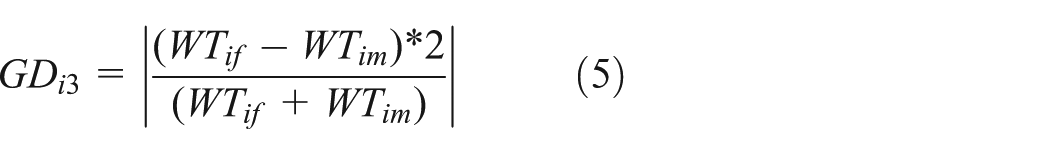
The equations to calculate GD_i2 and GD_i3 are traditional ways to calculate ‘relative change’ and ‘relative percentage difference’ between two values.² Unlike equation 3, GD_i2 and GD_i3 take into account the relative sizes of the distances compared. We therefore use these two measurements to evaluate commuting distance differences between members of a couple.

According to equations 4 and 5, these two dependent variables are restricted to bounded proportions between −2 and 2, and between 0 and 2 respectively. With these dependent variables, inference through ordinary least-squares regression would be problematic because the normality and homoscedasticity assumptions of the error term are usually untenable. In this study, we propose using a beta regression model and maximum likelihood estimation to investigate the relationship between the outcome variables and covariates. This model specification is useful for situations where the outcome variable is measured in a continuous scale but bounded by a known interval. The proposed model is based on the assumption that the dependent variable is beta distributed. The density of this distribution is very flexible and can have different shapes depending on the values of the distribution parameters (Ferrari and Cribari-Neto, 2012). This flexibility encourages its empirical use in a wide range of applications (Johnson, et al., 1995: 235).

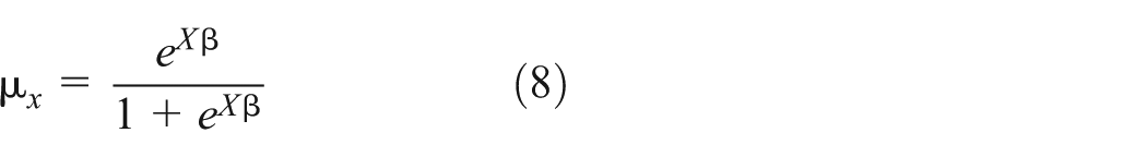
Mathematically, beta regression is used to simulate the mean of the dependent variable y (bounded by 0 and 1), conditional on covariates X , which we denote by $μ_{x}$ . We do this by using the link function for the conditional mean, denoted. g(•):³

g (μ_{x}) = X β

(6)

or equivalently,

μ_{x} = g^{- 1} (X β)

(7)

g ⁻¹ is the inverse link function of g(•). There are several possible choices for the link function. But a particularly useful link function is the logit link, which we can write as the following equation (see, for example, Ferrari and Cribari-Neto, 2012):

μ_{x} = \frac{e^{X β}}{1 + e^{X β}}

(8)

For bargaining power indicators, a large proportion of the research has proposed that the comparative resources of husband and wife have important influences on dyadic power differentials (McDonald, 1980; Warner, et al., 1986). In other words, the decision-making power of each spouse is directly dependent on the comparative degree to which that spouse contributes valued resources to the family (Warner et al., 1986). But methods for turning the theoretical notion of relative bargaining power into empirically implementable measurements have been the subject of controversy. Much of the existing literature focuses on economic indicators, including wage and nonwage income (Chau et al., 2007; Hoddinott and Haddad, 1995; Schultz, 1990; Thomas, 1990) and/or assets controlled by the couples’ members at time of marriage (Brown, 2009; Quisumbing and Maluccio, 2003; Thomas, et al., 1997; Zhang and Chan, 1999). Yet some of these measurements could be problematic as they may be endogenous to the outcome of interest in the studies (Li and Wu, 2011).

A valid measure of bargaining power should not only reflect relative bargaining positions between husband and wife but also be exogenous to outcomes under investigation (Li and Wu, 2011). In this paper, we use the following indicators to capture the array of dimensions that contribute to the relative bargaining power between members of a couple: age difference (Albrecht et al., 1979; Friedberg and Webb, 2006); respective education levels achieved by wife and husband, which includes the following possibilities: ‘power couple’⁴ (if both husband and wife received college or more education), low-power couple (if neither of them received college education), husband-powered couple (if only the husband received college or more education) and wife-powered couple (if only the wife received college or more education) (Orrefice and Bercea, 2006); Hukou (residency status)⁵ held by wife or husband, which has the following possibilities: ‘Beijing couple’ (if both husband and wife have Beijing Hukou), migrant couple (if neither has Beijing Hukou), only wife with Beijing Hukou and only husband with Beijing Hukou.

Using these indicators, we view ‘power’ as a multi-faceted concept. Each of the indicators of power captures a different dimension of the complex interaction that takes place between husband and wife (Beegle et al., 2001). More importantly, these indicators are either defined by nature (age difference), determined before marriage (education difference, for most people) or institutionalised at birth (Hukou status), which make them exogenous to the model specifications.

Godwin and Scanzoni (1989) propose that besides comparative resources of the husband and wife, partners’ emotional interdependence including ‘their degree of love and caring for their spouse’ and ‘their degree of commitment to the current marital relationship’ can play an important role in shaping each dyadic power relationship. However, the survey data in this study do not provide information to quantify these factors. These factors could meanwhile be directly related to individual income, education or other factors, which may make the degree of love, caring or commitment endogenous to the model (Fernandez and Guner, 2001; Folbre and Nelson, 2000). In this study, we leave ‘emotional dependence’ in the error term.

To quantify another important explanatory variable: institutional characteristics, we use housing property rights information and age categories to do this job. As discussed before, China has adopted since 1978 a series of urban housing reforms to privatise and commercialise the urban housing stock. After three decades of housing reforms in China, housing tenure in urban areas has undergone profound changes. Three major types of housing tenure can be identified in today’s urban housing market, differentiated by the source through which housing is obtained. The first type is subsidised homeownership for work unit (or state institution) housing properties, which were sold by work units or state institutions to current homeowners. The prices of these properties were not determined in an open market. Ownership of these properties can be seen as a relic of the old central planning regime and as representing ‘half-way privatisation’. The second type of tenure involves commercial housing properties sold by real estate developers without state subsidies. The third type consists of ‘social’ housing properties, heavily subsidised by local governments. This housing stock includes Economical and Comfortable Housing (ECH) and Cheap Rental Housing (CRH) under Chinese governmental programmes.

In terms of age categories, the sample population in this paper was divided into two groups by age as of 1 January 2010, with 33 years of age on that date being used as the dividing point. By using this cut-off, the individuals are identified as younger and older generation; and the couples are classified as three groups: 1) younger-generation couple if both wife and husband are 33 years old or younger at the time of the survey, 2) older-generation couple if both of them were older than 33 years old and 3) mixed-generation couple if the couple members overlapped these categories.

Our opening assumption was that the 1998 housing reform and 1997 education policy reform profoundly re-defined incentive structures among the sample and would systematically differentiate one group of individuals from another by age, which in turn could generate different influences on the job and housing location choices of these two groups. The older age cohort was more likely to already be employed in jobs, and live in housing allocated and/or assigned by the state or work units, while members of the younger group were more likely to rely on the market to find their own jobs and housing. In terms of access to housing properties and jobs, as men and women are treated differently under the socialist regime and the market-oriented reforms, bargaining power in families might well be changed under these two different institutional contexts. This change of economic regimes provides a ‘natural experiment’ to explore how commuting distance patterns changed for these two age cohorts.

Other family characteristics have been recognised to be possibly associated with the dependent variables. For example, such factors as family size, income level, the presence of young children and/or parents and car user-ship (wife and husband each has and uses a separate car, couple without car, only husband uses car and only wife uses car). Spatial characteristics of home and/or workplaces could be another category of factor to be taken into consideration for job and/or residential locational choices. We list these variables in Tables 1 and 2 as control variables.⁶

Table 1.

Descriptive statistics for all the observations.

Variable	Obs	Mean	Std. Dev.	Min	Max
DEPENDENT VARIABLE
Work trip distance (km)	51,941	7.385	8.234	0.001	79.444
Work trip distance for females (km)	24,322	6.861	7.771	0.001	79.444
Work trip distance for males (km)	27,619	7.847	8.595	0.001	78.910
INSTITUTION INDICATORS
Age category (= 1 if age < = 33 )	51,941	0.435	0.496	0	1
Commercial housing property	51,941	0.281	0.450	0	1
Subsidised homeownership by work unit	51,941	0.363	0.481	0	1
Rent	51,941	0.203	0.402	0	1
Social housing	51,941	0.046	0.209	0	1
Other housing properties¹	51,941	0.107	0.309	0	1
GENDER
Female ( Female = 1, Male = 0)	51,941	0.468	0.499	0	1
CONTROL VARIABLE
Age	51,941	36.984	10.389	18	59
Beijing Hukou (= 1 if yes, otherwise = 0)	51,941	0.769	0.422	0	1
High education (1 = college and more, 0 = otherwise)	51,941	0.372	0.483	0	1
Profession
Labour intensive job	50,406	0.098	0.297	0	1
Clerical support workers; Service and sales workers	50,406	0.552	0.497	0	1
Civil servants in government agencies or	50,406	0.151	0.358	0	1
SOEs; Armed forces occupations
Teaching professionals; Health professionals	50,406	0.075	0.264	0	1
Social workers; Self-employed; Private business people; and Other	50,406	0.058	0.234	0	1
Other professions	50,406	0.066	0.249	0	1
Use automobile by individual(1 = yes, 0 = no)	54,773	0.259	0.438	0	1
Single (1 = yes, 0 = no)	51,941	0.063	0.242	0	1
Annual income per capita (log value)	51,921	10.123	0.498	9.210	12.676
Number of people in family	51,941	2.840	0.985	1	5
Presence of senior people (1 = yes, 0 = no)	51,941	0.400	0.490	0	1
Number of children (under 6 years)	51,941	0.122	0.335	0	3
Number of children between 6 to 12 years old	51,941	0.101	0.307	0	3
Distance from home to Tian-An-Men (km)	51,941	15.334	13.870	0.311	79.054
Distance from workplace to Tian-An-Men (km)	51,941	14.280	14.147	0.136	107.449
Job opportunities (,000)	51,065	379.839	348.035	0.122	1135.7

Note: ¹Other housing properties include informal housing properties, self-constructed and self-use properties, properties with disputed or unclear property owners, etc.

Table 2.

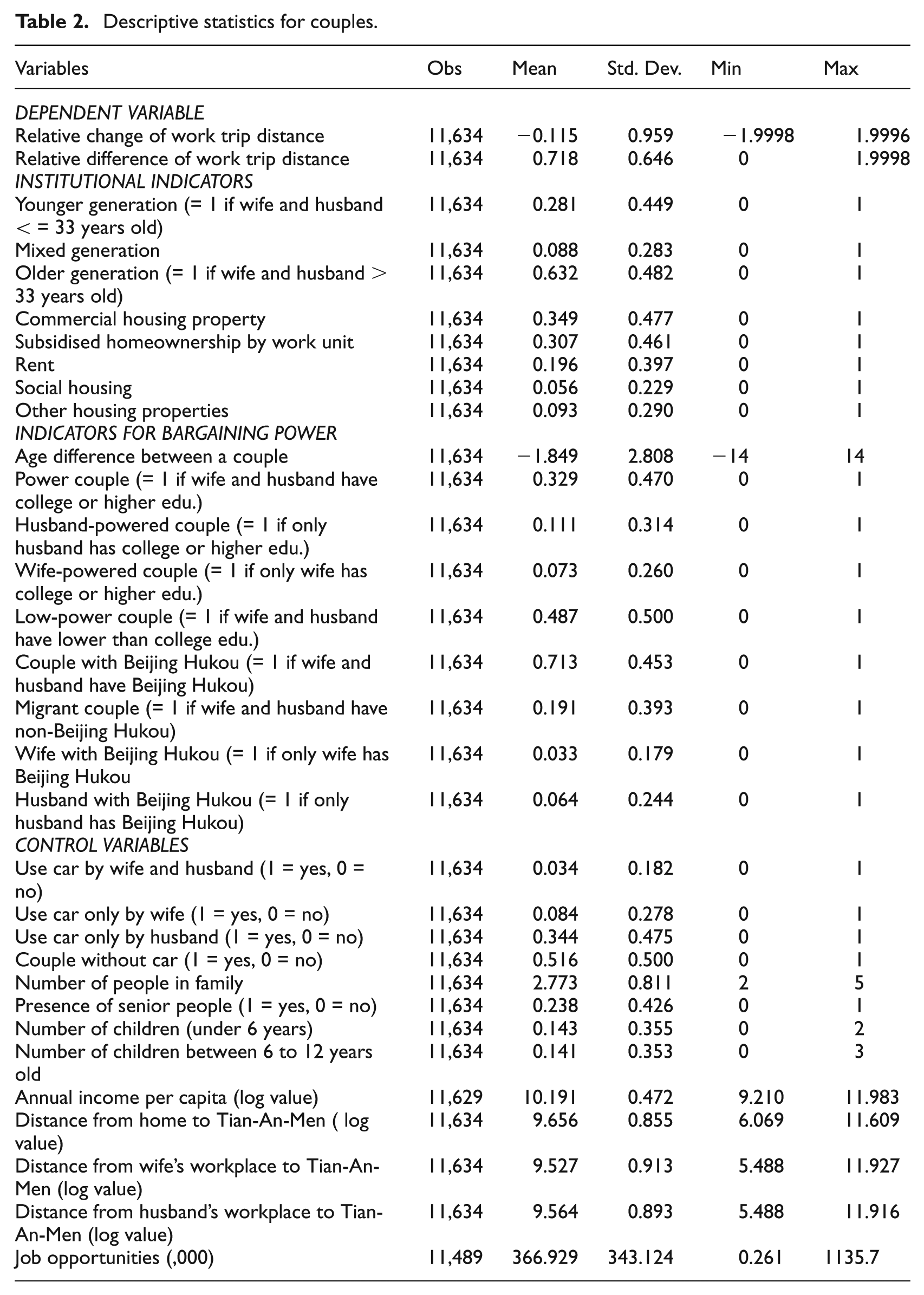
Descriptive statistics for couples.

Variables	Obs	Mean	Std. Dev.	Min	Max
DEPENDENT VARIABLE
Relative change of work trip distance	11,634	−0.115	0.959	−1.9998	1.9996
Relative difference of work trip distance	11,634	0.718	0.646	0	1.9998
INSTITUTIONAL INDICATORS
Younger generation (= 1 if wife and husband < = 33 years old)	11,634	0.281	0.449	0	1
Mixed generation	11,634	0.088	0.283	0	1
Older generation (= 1 if wife and husband > 33 years old)	11,634	0.632	0.482	0	1
Commercial housing property	11,634	0.349	0.477	0	1
Subsidised homeownership by work unit	11,634	0.307	0.461	0	1
Rent	11,634	0.196	0.397	0	1
Social housing	11,634	0.056	0.229	0	1
Other housing properties	11,634	0.093	0.290	0	1
INDICATORS FOR BARGAINING POWER
Age difference between a couple	11,634	−1.849	2.808	−14	14
Power couple (= 1 if wife and husband have college or higher edu.)	11,634	0.329	0.470	0	1
Husband-powered couple (= 1 if only husband has college or higher edu.)	11,634	0.111	0.314	0	1
Wife-powered couple (= 1 if only wife has college or higher edu.)	11,634	0.073	0.260	0	1
Low-power couple (= 1 if wife and husband have lower than college edu.)	11,634	0.487	0.500	0	1
Couple with Beijing Hukou (= 1 if wife and husband have Beijing Hukou)	11,634	0.713	0.453	0	1
Migrant couple (= 1 if wife and husband have non-Beijing Hukou)	11,634	0.191	0.393	0	1
Wife with Beijing Hukou (= 1 if only wife has Beijing Hukou	11,634	0.033	0.179	0	1
Husband with Beijing Hukou (= 1 if only husband has Beijing Hukou)	11,634	0.064	0.244	0	1
CONTROL VARIABLES
Use car by wife and husband (1 = yes, 0 = no)	11,634	0.034	0.182	0	1
Use car only by wife (1 = yes, 0 = no)	11,634	0.084	0.278	0	1
Use car only by husband (1 = yes, 0 = no)	11,634	0.344	0.475	0	1
Couple without car (1 = yes, 0 = no)	11,634	0.516	0.500	0	1
Number of people in family	11,634	2.773	0.811	2	5
Presence of senior people (1 = yes, 0 = no)	11,634	0.238	0.426	0	1
Number of children (under 6 years)	11,634	0.143	0.355	0	2
Number of children between 6 to 12 years old	11,634	0.141	0.353	0	3
Annual income per capita (log value)	11,629	10.191	0.472	9.210	11.983
Distance from home to Tian-An-Men ( log value)	11,634	9.656	0.855	6.069	11.609
Distance from wife’s workplace to Tian-An-Men (log value)	11,634	9.527	0.913	5.488	11.927
Distance from husband’s workplace to Tian-An-Men (log value)	11,634	9.564	0.893	5.488	11.916
Job opportunities (,000)	11,489	366.929	343.124	0.261	1135.7

Data and results

Data

The data used in this study comes from the Beijing Household Travel Survey (BHTS), conducted in September and October 2010 by the Beijing Transportation Research Center (BTRC). In order to develop a representative sample, the survey used a multi-stage cluster strategy to select a sample from the target population. In the survey, the study area was first divided into 388 communities and 1911 neighbourhoods, from which 233 communities were randomly selected. Then 1085 neighbourhoods in these 233 communities were randomly selected based on the list provided by the municipal government. In each neighbourhood, 10 to 50 households were randomly selected, according to the size of the neighbourhood, for face-to-face interviews with each household member to complete the survey questionnaires. The final sample size was 46,900 households, with a total of 116,142 respondents, all in the Beijing Municipal Area. The survey sample accounted for 0.59 percent of the total population of the Beijing Municipal Area. This ratio is roughly consistent across different districts. Average household size for the survey was 2.48 persons per household, slightly higher than is reflected in Beijing census data (2.45 persons per household). The male sample in the survey is 55,577, and the female sample is 60,565, accounting for 47.85 percent and 52.15 percent of the total sample, respectively. Compared with Beijing census data, which had a 51.6 percent male population, the survey has a higher female representation (BTRC, 2011).

For the purpose of this analysis, the sample was restricted to those persons who were employed and worked away from home at the time of the survey, and who provided both home and work addresses. Out of total of 116,142 respondents, this left 51,941 individuals with valid trip distance information in 31,987 families, of which there were 11,634 couples.

Table 1 provides definitions and descriptive statistics for the variables for all individuals in the sample. It shows that on average, the work trip distance for women is shorter than for men. About 43.5 percent of the sample of individuals used in this study belonged to the younger generation. Homeownership rate for our sample was 64.4 percent, in which ‘subsidised homeownership by work units’ takes the largest share.

Table 2 provides description and general statistics for the variables that we use in this study to analyse bargaining power between wives and husbands. Among all of the couples in the sample, about 28.1 percent are categorised as younger generation. We can also see from Tables 1 and 2 that married couples are more likely to reside in commercial housing properties. In the couple sample, about 32.9 percent of the couples reported college and higher education for both wives and husbands, while 48.7 percent of couples had less than college educations. Couples who were both migrants without Beijing Hukou accounted for 19.1 percent of the total, while 71.3 percent of the couples had Beijing Hukou for both spouses.

Empirical results

By using GLM models, we put male and female observations together to generate exponentiated coefficients for the covariates listed in Table 3. A coefficient larger than 1 indicates the probability that the corresponding covariate is positively correlated with the dependent variable, and vice versa for the coefficients smaller than 1.

Table 3.

Work trip distance analysis result (GLM Regression).

Variables	All Observations	Female Observations	Male Observations
Female ( Female = 1, Male = 0)	0.862***
	(0.009)
Institution Indicators
Age category (= 1 if age < = 33 )	1.078***	1.075**	1.054**
	(0.021)	(0.033)	(0.027)
Commercial housing property	1.082***	1.032	1.127***
	(0.015)	(0.021)	(0.021)
Rent	0.868***	0.834***	0.901***
	(0.015)	(0.021)	(0.020)
Social housing	1.068***	1.052	1.084***
	(0.022)	(0.032)	(0.030)
Other housing properties	0.900***	0.885***	0.913***
	(0.018)	(0.027)	(0.024)
Control Variables
Age	0.992***	0.989***	0.994***
	(0.001)	(0.002)	(0.001)
Beijing Hukou (= 1 if yes, otherwise = 0)	1.094***	1.067***	1.126***
	(0.016)	(0.023)	(0.022)
High education (1 = college and more, 0 = otherwise)	1.131***	1.146***	1.122***
Profession	(0.012)	(0.018)	(0.016)
Clerical support workers; Service and sales workers	1.202***	1.242***	1.188***
	(0.025)	(0.050)	(0.029)
Civil servants in government agencies or SOEs; Armed	0.971	1.035	0.941**
forces occupations	(0.023)	(0.046)	(0.027)
Teaching professionals; Health professionals	0.937**	1.002	0.851***
	(0.026)	(0.045)	(0.037)
Social workers; Self-employed; Private businesspeople; and	0.836***	0.810***	0.860***
Other	(0.027)	(0.046)	(0.034)
Other professions	0.841***	0.798***	0.903**
	(0.027)	(0.042)	(0.036)
Annual income per capita (log value)	1.107***	1.151***	1.081***
	(0.015)	(0.023)	(0.020)
Use automobile by individual(1 = yes, 0 = no)	1.139***	1.194***	1.104***
	(0.014)	(0.024)	(0.016)
Number of people in family	1.013	1.019	1.008
	(0.009)	(0.014)	(0.012)
Presence of senior people (1 = yes, 0 = no)	1.123***	1.124***	1.120***
	(0.015)	(0.023)	(0.020)
Number of children (under 6 years)	1.001	0.987	1.012
	(0.017)	(0.027)	(0.023)
Number of children between 6 to 12 years old	0.990	0.952*	1.027
	(0.019)	(0.026)	(0.026)
Single (1 = yes, 0 = no)	0.862***	0.880***	0.845***
	(0.021)	(0.032)	(0.027)
Distance from home to Tian-An-Men (log value)	1.075***	1.090***	1.061**
	(0.020)	(0.030)	(0.026)
Distance from workplace to Tian-An-Men (log value)	1.043***	1.012	1.071***
	(0.009)	(0.013)	(0.011)
Job opportunities (bike distance, log value)	0.945***	0.925***	0.959***
	(0.006)	(0.009)	(0.008)
Control districts	Yes	Yes	Yes
Number of observations	49,538	23,350	26,188
Log pseudolikelihood	−145,484.6	−66,467.4	−78,878.1
Pearson	59,615.8	29,918.5	29,568.8
Deviance	57,946.4	27,112.8	30,555.5
AIC	5.875	5.697	6.027

Notes: Coefficients are exponentiated coefficients. Standard errors are in parentheses. * p < 0.10, ** p < 0.05, *** p < 0.01.

The established research literature consistently shows that women have shorter commutes than men. Beijing is not an exception. Table 3 shows that female residents in Beijing had significantly shorter commute distances than male residents. The findings further show that the younger generation, especially younger females, had longer average trip distances between residential and work locations than the older generation. Compared with those living in subsidised work unit (or state institution) housing properties, people who owned and lived in commercial housing or lived in social housing units, especially the males, had longer work trip distances, while renters tended to travel shorter distances to their workplaces.

In line with previous findings, residents with higher incomes, higher education levels and who had cars, both men and women, tended to travel longer distances to work. For families with senior people at home, both men and women tend to have longer commute trips, all other factors being equal. The Chinese traditional multi-generational family may play a role in this trend. It is normal in China for parents to live with married children under the same roof. For these families, the older generation usually provides substantial help in taking care of household work and children, especially pre-school children. This help can reduce the household responsibilities of housewives, which in turn may explain the insignificant coefficients for the presence of children in the models.

As shown in Table 3, clerical, service and sales workers lived further from their work places on average than workers in the labour intensive industrial and agricultural sectors. Another two occupational categories meriting attention are the ‘Civil servants in government or SOEs, or the armed forces’, and ‘Teaching and health professionals’. People in these occupations were usually assured lifelong jobs and work unit housing properties. Work unit residences are generally close to workplaces, and housing was more often assigned to men. Table 3’s results corroborate that men in these two types of occupations were more likely in general, and more likely than women in these occupations, to work near home.

Table 3 also shows that living or working close to the Beijing city centre typically reduces commute distances for men and women. Yet in terms of work trip distance, home location matters more for women, while job location has stronger associations with work trip distance for men. Table 3 also shows that, controlling for other variables, more job opportunities near homes are correlated with shorter commute distances, especially for women, who may be more likely to take advantage of work nearby and less likely to hold out for more desirable jobs ‘downtown’.

In Table 4, the marginal effects for ‘relative change of work trip distance’ and ‘relative difference of work trip distance’ are derived from beta regressions. These marginal effects depend on the values of the independent variables. Those displayed in Table 4 are for a fictional observation whose explanatory variables are fixed at the mean or at values specified as 0 for dummy variables.

Table 4.

Regression results for couples.

	Relative change of work trip distance¹			Relative difference of work trip distance¹
	Model 1	Model 2	Model 3	Model 4	Model 5	Model 6
Variables	All Observation	Old generation	Young generation	All Observation	Old generation	Young generation
Institution Indicators
Younger generation	0.009			−0.039***
	(0.0061)			(0.0079)
Mixed generation	0.009			−0.039***
	(0.0091)			(0.0116)
Commercial housing property	−0.023***	−0.026**	−0.037**	−0.046***	−0.059***	−0.013
	(0.0063)	(0.0079)	(0.0133)	(0.0079)	(0.0096)	(0.0164)
Rent	−0.022**	−0.019	−0.036**	0.021*	0.005	0.045*
	(0.0079)	(0.0114)	(0.0139)	(0.0106)	(0.0146)	(0.018)
Social housing	−0.014	−0.012	−0.017	−0.063***	−0.074***	−0.009
	(0.0106)	(0.0131)	(0.0226)	(0.0132)	(0.0156)	(0.0277)
Other housing properties	−0.025**	−0.026*	−0.043*	−0.001	−0.001	−0.007
	(0.0092)	(0.0112)	(0.0205)	(0.0124)	(0.0144)	(0.0263)
Bargaining Power
Age difference between a couple	−0.001	−0.002	0.001	0.0003	0.001	0.001
	(0.0009)	(0.0011)	(0.002)	(0.0012)	(0.0014)	(0.0025)
Power couple	−0.001	0.0003	−0.011	0.002	0.001	−0.001
	(0.0059)	(0.0084)	(0.0104)	(0.0078)	(0.0104)	(0.0136)
Husband-powered couple	−0.011	−0.009	−0.009	−0.006	−0.001	−0.003
	(0.0077)	(0.01)	(0.0153)	(0.0099)	(0.0122)	(0.0192)
Wife-powered couple	−0.007	−0.024*	0.022	−0.009	0.023	0.001
	(0.0094)	(0.012)	(0.0172)	(0.0119)	(0.0142)	(0.0217)
Migrant couple	0.017*	0.020	0.023*	−0.042***	−0.056***	−0.044**
	(0.0073)	(0.0113)	(0.0113)	(0.01)	(0.0156)	(0.0142)
Wife with Beijing Hukou	−0.019	0.011	−0.048**	−0.035*	0.038	−0.023
	(0.0135)	(0.0232)	(0.0177)	(0.0168)	(0.0285)	(0.0211)
Husband with Beijing Hukou	0.029**	0.003	0.046***	−0.022	0.017	−0.004
	(0.0099)	(0.0173)	(0.0136)	(0.0125)	(0.0216)	(0.0167)
Control Variables
Number of people in family	0.001	0.003	0.018	−0.008	−0.001	−0.019
	(0.0045)	(0.0057)	(0.0116)	(0.006)	(0.0072)	(0.0151)
Use automobile only by wife (1 = yes, 0 = no)	0.048***	0.038***	0.042*	0.003	0.021	−0.005
	(0.0087)	(0.0113)	(0.0167)	(0.0112)	(0.0136)	(0.0211)
Use automobile only by husband (1 = yes, 0 = no)	−0.018***	−0.022**	−0.07	−0.013	−0.008	−0.014
	(0.0052)	(0.0069)	(0.0096)	(0.0068)	(0.0085)	(0.0123)
Use automobile by husband and wife (1 = yes, 0 = no)	0.018	−0.001	−0.0003	−0.045*	−0.015	−0.041
	(0.0135)	(0.0161)	(0.0303)	(0.0175)	(0.0202)	(0.0357)
Presence of senior people (1 = yes, 0 = no)	−0.005	−0.003	−0.019	−0.009	−0.009	0.027
	(0.0065)	(0.0075)	(0.0204)	(0.0086)	(0.0098)	(0.0277)
Number of children (under 6 years)	−0.003	−0.001	−0.021	0.011	0.005	0.013
	(0.0081)	(0.0128)	(0.0155)	(0.0107)	(0.0161)	(0.0203)
Number of children between 6 to 12 years old	0.001	0.002	0.001	0.004	0.010	0.027
	(0.0073)	(0.0084)	(0.0245)	(0.0096)	(0.0104)	(0.0357)
Annual income per capita (log value)	0.004	0.011	0.011	−0.022**	−0.024*	−0.019
	(0.0066)	(0.0095)	(0.0108)	(0.0079)	(0.0113)	(0.012)
Distance from home to Tian-An-Men (log value)	0.015**	0.019**	0.013	−0.025**	−0.013	−0.015
	(0.0059)	(0.0078)	(0.0106)	(0.007)	(0.0098)	(0.0122)
Distance from wife’s workplace to Tian-An-Men	−0.007	−0.006	−0.034***	0.028***	0.024***	0.046***
(log value)	(0.0042)	(0.0054)	(0.0068)	(0.0056)	(0.0063)	(0.0104)
Distance from husband’s workplace to Tian-An-	−0.008	−0.013*	0.026***	0.044***	0.04***	0.051***
Men (log value)	(0.004)	(0.0048)	(0.0065)	(0.0057)	(0.006)	(0.0105)
Job opportunities (bike distance, log value)	−0.007*	−0.005	−0.003	0.016***	0.008	0.012
	(0.0028)	(0.0036)	(0.0054)	(0.0041)	(0.0047)	(0.0076)
Number of observations	10726	7212	3261	8518	5793	2647
Log likelihood	929.167	275.612	262.984	651.697	184.956	229.996
ln_Phi	1.233***	1.005***	1.201***	0.720***	0.639***	0.677***
	(0.0121)	(0.0145)	(0.0219)	(0.0131)	(0.0156)	(0.0234)

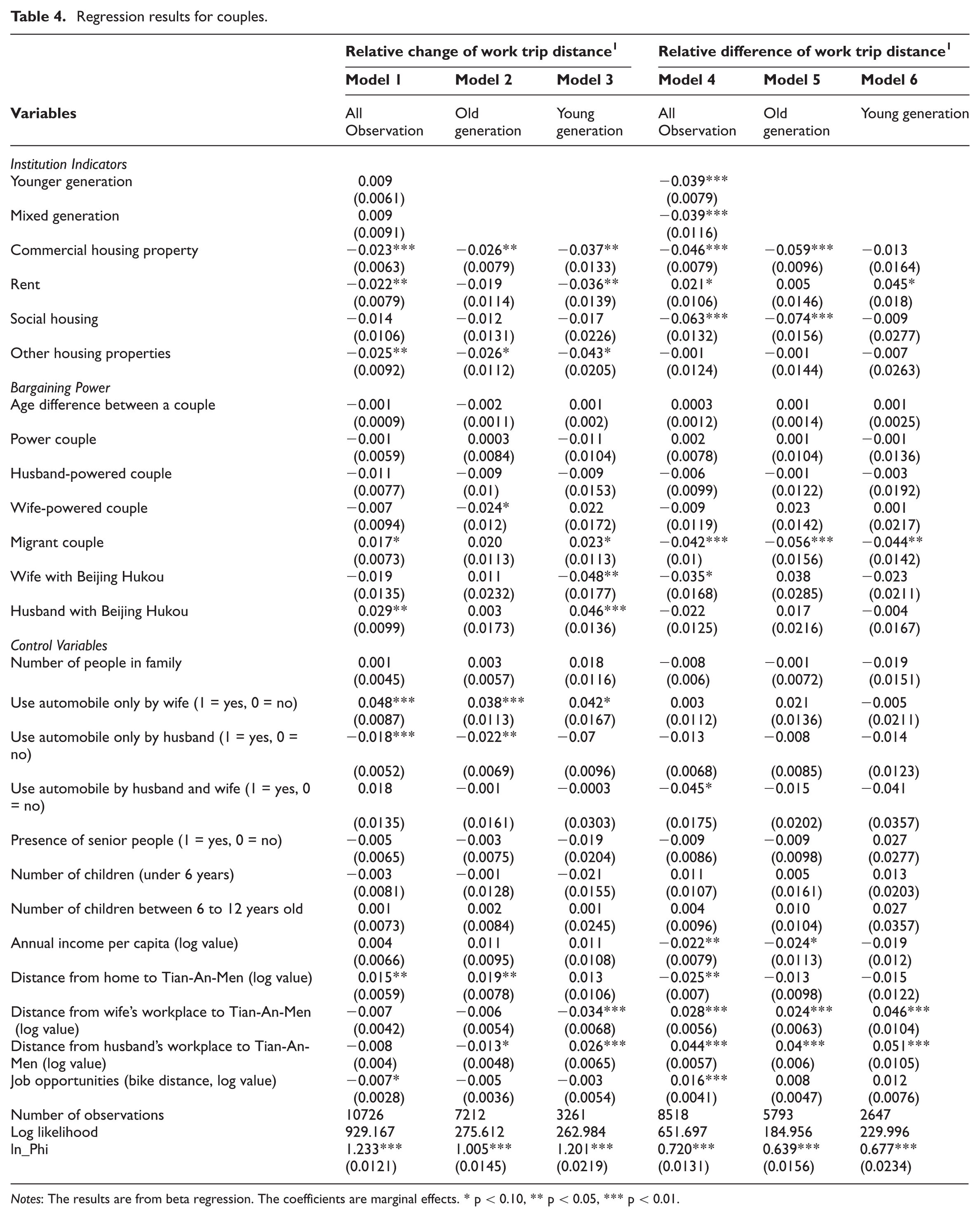
Notes: The results are from beta regression. The coefficients are marginal effects. * p < 0.10, ** p < 0.05, *** p < 0.01.

There are several issues need to be clarified to help us understand the results in Table 4. First, the spatial boundary of Beijing Metropolitan Area has been expanded in the last several decades. As the existing physical constructions in this city already occupied the spaces in the central area, the new constructions have largely taken place in the suburban area of Beijing. With these developments, people and jobs came. This is probably even more so for young people, as the older generation is more likely to take spaces in the central area for longer periods of time. Yet, the spatial distribution of the jobs in Beijing is still highly centralised (Sun et al., 2012). Under this spatial structure, young people would, on average, be more likely to have longer commutes than the older generation. Our data corroborate that the average commute distances for the younger generation and the older generation were 8.27km and 6.25km respectively. Second, as commute is inevitably associated with time and monetary cost, a shorter commute is then regarded as a benefit in this paper. We take the traditional assumption in the Economics field that the individual is a rational human being looking to maximise her benefit. The person with stronger bargaining power is then more likely to take a shorter commute. Third, the concept of ‘gender equality of trip distance’ will be used to interpret the results derived from ‘relative difference of work trip distance’ (GD_i₃ see equation 5). The zero value of GD_i₃ indicates a perfect gender equality of trip distance. In this case, wife and husband had the same commute distance. The maximum value of GD_i₃ indicates that either wife or husband had their workplace right by their home, while the other partner needed to travel a certain distance to her/his workplace. Gender equality of work trip distance might not be necessarily associated with a shorter commute or stronger bargaining power for one partner of a couple. Yet, given the fact that, on average, women travel shorter distances to workplaces than men do, the higher degree of gender equality of trip distance for a certain group of married women might indicate that this group of people value their jobs more than average.

Table 4 does show that the younger generation in Beijing has achieved a higher degree of gender equality of trip distance, as indicated by a negative and significant coefficient for the variable of ‘younger generation’ in Model 4. On average, the longer commutes taken by wives were getting closer to those of their husbands. Compared with the older generation, women in the younger generation were probably more likely to put more emphasis on their jobs.

For the second institution indicator – housing property rights – the results from Models 1 to 3 reveal that female residents in commercial housing properties tend to have much shorter commute distances than their husbands, as compared with couples in subsidised housing properties in work units. This could be explained by comparatively shorter commutes for wives and/or longer commutes for husbands in commercial housing properties as compared with their counterparts in subsidised housing properties. In the data, the average commute distances for wives and husbands in commercial properties were 7.8 km and 9.4 km respectively. For wives and husbands in subsidised housing properties, these numbers are 5.8 km and 6.6 km respectively. Of course, these average numbers and the differences between these numbers can be explained by factors other than housing property rights. They could, nevertheless, give us the most direct information to understand the regression results in Table 4.

Results in Table 4 also show that, compared with the couples in subsidised housing properties in work units, couples who lived in commercial housing properties had a smaller ‘relative difference of work trip distance’ (see the negative and significant coefficient for variable of ‘commercial housing property’ in Model 4). This trend is true for the older generation who lived in commercial properties (Model 5), but not for younger generation. Unlike the older generation who lived in subsidised housing properties in work units, older generation husbands or wives who lived in commercial housing properties are less likely to be affected by one ‘benefit’ of the welfare package provided by work units: potentially shorter commute distances. The difference of gender equality between older generations in subsidised housing properties vs. commercial housing properties then became significant, as indicated by Model 5. By contract, the difference of gender equality for the younger generation in subsidised housing properties vs. commercial housing properties is not significant (see Model 6). In our data, about 30.9 percent of the younger generation lived in subsidised work unit housing properties, either with parents who were employees of their work units, or inherited from parents or relatives or in some cases as purchasers of work unit housing units from previous owners. Unlike the older generation, however, these younger residents do not necessarily take jobs in the work units where they live. The results indicate that, once people have freedom to choose where they live or where they work, they would be less likely to be exposed to the systematic difference induced by the central planning system vs. the market-oriented job-housing distribution system in China.

In terms of bargaining power indicators, age difference does not show a significant influence on relative change/difference of commute distances between men and women. But education and Hukou do. Table 4 shows that wives in wife-powered couples tend to take relatively shorter work trips than their husbands, especially more so for the older generation. The significant and negative coefficient for ‘wife-powered couple’ in Model 2 indicates that if the wife has more education than her husband in an older-generation household, she is even more likely to live closer to her workplace. Education counts significantly as a factor to explain work trip distance for older generation wives.

By contrast, Hukou shows more significant influence than education for the younger generation. The wives in migrant couples tended to take relatively longer work trips than the wives in couples where both partners have Beijing Hukou. This is even more so for the younger generation, as indicated by the positive and significant coefficients for the variable of ‘migrant couples’ in Model 3. The gender equality of trip distance is also more readily achieved for the migrant couples (see Model 4, 5 and 6). Compared with couples in which both partners have Beijing Hukou, if it is only the wife or husband who had Beijing Hukou, she or he tended to have a shorter commute distance relative to her/his partner. This trend is only true for the younger generation (see Model 3). In other words, the younger generation with Beijing Hukou seems to have a stronger bargaining power to benefit from shorter commute distances.

In our view, if bargaining power works, this power should be exemplified by or executed through effective bargaining chips held by individuals. In pre-reform China, the state strictly controlled population movement. It was extremely difficult to get permission to change jobs or residential locations during that period. Hukou would be less likely to play a significant role in shaping bargaining power for the older generation. When the central-planning regime left little freedom to individuals, education became one of the very few resources that could be effectively controlled by individuals. This probably explains the significant effect of education in shaping bargaining power for the older generation. After economic reform, migration increasingly became a norm for people who tried to seek better opportunities outside their home towns. With this flow of population, differences between people with and without local Hukou became very meaningful. Especially in a city like Beijing, local Hukou is very valuable because it carries rights to a rich array of social benefits while the supply of which is severely restricted, which probably explains the significant effect this factor has for the younger generation.

Other findings include evidence that, once a wife or husband has a car, she/he commutes relatively longer than her/his counterpart in couples where neither partner has a car, as inferred by significant coefficients of corresponding covarites in Models 1 to 3.

Models 4 and 5 show that older-generation households with higher income levels tend to have a higher degree of commute distance equality between wives and husbands. For younger-generation households, intra-household gender equality is not significantly different for different income levels.

The distance of a couple’s home from the city centre is also a fairly significant factor. Table 4 shows that when residences are further from Beijing city centre, wives travel relatively longer distances to workplaces compared with families that are closer to the city centre (see Models 1 and 2). Wives or husbands working close to the city centre tend to travel relatively longer to their workplaces than their partners who work further from the city centre. The intra-family inequality of the work trip distances between wives and their husbands is getting larger, with longer distances from the wife’s or husband’s workplace to the city centre. These trends are more pronounced for the younger generation (see Models 3 to 6).

As shown in Table 4, more job opportunities around homes do not show much significant effect on the structure of trip distances between members of a couple. Especially for young couples, more jobs near home do not appear to reduce work trip distances for women.

Conclusion

In urban economics, the traditional model of location and land use developed by Alonso (1964) treats the household as if it behaves as a single and rational individual to maximise household benefit. Yet, a household is constituted of multiple members who may have different, sometimes even conflicting, preferences and interests. To the best of our knowledge, this study is the first empirical research in the urban studies field to take into account the specific intra-household coordination problems that arise due to the inevitable diversity of preferences and interests between spouses, and to shed light on intra-household arrangements with respect to commuting patterns in an urban area.

To do this, we used a large sample from the Beijing Household Travel Survey to build husband-wife dyads, construct variables to measure bargaining power between spouses and put intra-household travel pattern arrangements within a macro-level institutional transformation framework to analyse whether, and to what degree, institutions and bargaining power shape the travel patterns of married men and women.

The empirical results reveal that bargaining power does matter for intra-household travel pattern arrangements. They also suggest how macro-level institutions set limits to such bargaining and define which resources can be effective bargaining chips for individuals.

The results reveal that on average women have shorter commutes than men in Beijing. After economic reforms, women got more freedom to negotiate for their interests on a more equal footing within families than before. The findings corroborate that older-generation women – who are more likely to have been involved in central-planning institutional arrangements – tend to have shorter commute distances if they obtained more extensive educations than their husbands. In a stagnant, poor and egalitarian pre-reform regime, education became a relatively effective bargaining chip for older-generation women, compared with other resources, if there were any.

After economic reform, distribution of housing and jobs through markets became a norm for urban residents. People generally, and especially women (who historically had a more passive role), are playing more active roles than previous generations in deciding whether and where to buy homes and find jobs. The study shows that younger-generation women, once they hold or have more say over valuable resources, such as housing properties and Hukou, are more likely to arrange daily travel arrangements in their favour.

The spatial relationship between home and workplace has been, and remains, a core part of urban economics theories. Indeed, it is the separation of jobs, shops and home that largely produces trips in cities and shapes the landscapes of urban communities (Clark and Kuijpers-Linde, 1994; Quigley and Weinberg, 1977). Yet, as job and residential locational choices are two of the most important ones made by individual households, and commuting can be viewed as a derived demand to accommodate job and home-based duties, existing research literature on the job-housing spatial relationship provides very little information on intra-household behavioural responses to job-housing locational choices. Little is known as to how individual household members behave in choosing the job and residential locations that establish their commute patterns. We hope that this study can facilitate a better understanding of micro-level individual intra-household behavioural responses on commute arrangements as well as the influences macro-level institutional transformations have on such individual choices.

Footnotes

Funding

This paper received funding from the National Science Foundation of China 71403279.

Notes

References

Abraham

Nisic

(2012) A simple mobility game for couple’s migration decisions and some quasi-experimental evidence. Rationality and Society 24(2): 168–197.

Agarwal

(1997) ‘Bargaining’ and gender relations: Within and beyond the household. Feminist Economics 3(1): 1–51.

Albrecht

Bahr

Chadwick

(1979) Changing family and sex roles: An assessment of age differences. Journal of Marriage and Family 41: 41–50.

Alonso

(1964) Location and Land Use. Cambridge, MA: Harvard University Press.

Becker

(1981) Treatise on the Family. Cambridge MA: Harvard University Press.

Beegle

Frankenberg

Thomas

(2001) Bargaining power within couples and use of prenatal and delivery care in Indonesia. Working paper.

Beijing Transportation Research Center (2011) Travel survey for the residents in Beijing. Research report.

Blumen

(1994) Gender differences in the journey to work. Urban Geography 15(3): 223–245.

Brown

(2009) Dowry and intra-household bargaining: Evidence from China. Journal of Human Resources 44(1): 25–46.

10.

Brun

Fagnani

(1994) Lifestyles and locational choices–Trade-offs and compromises: A case-study of middle-class couples living in the Ile-de-France region. Urban Studies 31: 921–934.

11.

Chau

Liu

. (2007) Testing the collective model of household labor supply: Evidence from China. China Economic Review 18(4): 389–402.

12.

Chen

Guo

(2011) One decade of urban housing reform in China: Urban housing price dynamics and the role of migration and urbanization, 1995–2005. Habitat International 35: 1–8.

13.

Clark

WAV

Kuipjers-Linde

(1994) Commuting in restructuring urban regions. Urban Studies 31: 465–483.

14.

Costa

Kahn

(2000) Power couples: Changes in the locational choice of the college educated, 1940–1990. The Quarterly Journal of Economics 115(4): 1287–1315.

15.

Deng

Shen

Wang

(2011) The emerging housing policy framework in China. Journal of Planning Literature 26(2): 168–183.

16.

Fernandez

Guner

(2001) Love and money: A theoretical and empirical analysis of household sorting and inequality. Working paper. Available at: http://parc.pop.upenn.edu/sites/parc.pop.upenn.edu/files/parc/PARCwps01–02.pdf.

17.

Ferrari

SLP

Cribari-Neto

(2012) Beta Regression for Modelling Rates and Proportions. Available at: http://orfe.princeton.edu/∼alaink/NJ_aTaxiOrf467F12/Papers/Machine%20Learning/beta.pdf.

18.

Folbre

Nelson

(2000) For love or money–Or both. Journal of Economic Perspectives 14(4): 123–140.

19.

Friedberg

Webb

(2006) Determinants and Consequences of Bargaining Power in Households. NBER working paper. Available at: http://www.nber.org/papers/w12367.pdf.

20.

Godwin

Scanzoni

(1989) Couple consensus during marital joint decision-making: A context, process, outcome model. Journal of Marriage and Family 51(4): 943–956.

21.

Goldin

(2006) The quiet revolution that transformed women’s employment, education, and family. American Economic Review 96(2): 1–21.

22.

Hanson

(1980) Gender and urban activity patterns in Uppsala, Sweden. Geographical Review 70: 291–299.

23.

Hanson

Johnston

(1985) Gender differences in work-trip length: Explanations and implications. Urban Geography 6(3): 193–219.

24.

Hanson

Pratt

(1990) Geographic perspectives on the occupational segregation of women. National Geographic Research 6(4): 376–399.

25.

Hoddinott

Haddad

(1995) Does female income share influence household expenditures? Evidence from Cote D’Ivoire. Oxford Bulletin of Economics and Statistics 57(1): 77–96.

26.

Johnson

Kotz

Balakrishnan

(1995) Continuous Univariate Distributions. Vol. 2. New York: Wiley.

27.

Johnston-Anumonwo

(1992) The influence of household type on gender differences in work trip distance. Professional Geographer 44(2): 161–169.

28.

(2011) Gender of children, bargaining power, and intra-household resource allocation in China. Journal of Human Resources 46(2): 295–316.

29.

Ligon

(2002) Dynamic Bargaining in Households (with application to Bangladesh). CUDARE Working Paper Series 972, Department of Agricultural and Resource Economics and Policy, University of California at Berkeley, USA.

30.

Lundberg

Pollak

(2003) Efficiency in marriage. Review of Economics of the Household 1(3): 153–167.

31.

McDonald

(1980) Family power: The assessment of a decade of theory and research, 1970–1979. Journal of Marriage and Family 42(4): 841–854.

32.

McLafferty

Preston

(1991) Gender, race, and commuting among service sector workers. The Professional Geographer 43(1): 1–15.

33.

Madden

(1981) Why women work close to home. Urban Studies 18: 181–194.

34.

Manning

Mullahy

(2001) Estimating log models: To transform or not to transform?Journal of Health Economics 20(4): 461–494.

35.

Manning

Basu

Mullahy

(2005) Generalized modeling approaches to risk adjustment of skewed outcomes data. Journal of Health Economics 24(3): 465–488.

36.

Michelson

(1988) Divergent convergence: The daily routines of employed spouses as a public affairs agenda. In: Andrew

Milroy

(eds) Life Spaces: Gender, Household, Employment. Vancouver: University of British Columbia Press, pp. 81–101.

37.

Orrefice

Bercea

(2006) Quality of Available Mates, Education and Intra-Household Bargaining Power. SSRN working paper. Available at: http://papers.ssrn.com/sol3/papers.cfm?abstract_id=944469.

38.

Pinch

Storey

(1992) Labour-market dualism: Evidence from a survey of households in the Southampton city-region. Environment and Planning A 24(4): 571–589.

39.

Pratt

Hanson

(1991) Time, space, and the occupational segregation of women: A critique of Human Capital Theory. Geoforum 22: 149–157.

40.

Quigley

Weinberg

(1977) Intro-urban residential mobility: A review and synthesis. International Regional Science Review 2: 41–66.

41.

Quisumbing

Maluccio

(2003) Resources at marriage and intra-household allocation: Evidence from Bangladesh, Ethiopia, Indonesia, and South Africa. Oxford Bulletin of Economics and Statistics 65(3): 283–328.

42.

Rai

(1994) Gender issues in China: A survey. Journal of China Report 30(4): 407–420.

43.

Robinson

(1985) Of women and washing machines: Employment, housework, and the reproduction of motherhood in socialist China. The China Quarterly 101: 32–57.

44.

Robinson

(1988) Who’s doing the housework?American Demographics 10(12): 24–28.

45.

Schultz

(1990) Testing the neoclassical model of family labor supply and fertility. Journal of Human Resources 25(4): 599–634.

46.

Sen

(1987) Gender and Cooperative Conflicts. WIDER working papers.

47.

Shelton

Daphne

(1993) Does marital status make a difference? Housework among married and cohabiting men and women. Journal of Family Issues 14(3): 401–420.

48.

Sun

Wang

(2012) Distributions of population and employment, and evolution of spatial structures in the Beijing Metropolitan Area. Acta Geographica Sinica 67(6): 829–840. [In Chinese].

49.

Thomas

(1990) Intra-household resource allocation: An inferential approach. The Journal of Human Resources 25(4): 635–664.

50.

Thomas

Contreras

Frankenburg

(1997) Distribution of Power Within the Household and Child Health. Santa Monica, CA: RAND Corporation.

51.

Turner

Niemeier

(1997) Travel to work and household responsibility: New evidence. Transportation 24: 397–419.

52.

Wang

(2011) Protection of Housing Property Rights for Divorced Women. Available at: http://www.yzfl.org/detail.php?n=108319&c=90080. [In Chinese].

53.

Wang

Murie

(1996) The process of commercialisation of urban housing in China. Urban Studies 33: 971–989.

54.

Warner

Lee

(1986) Social organization, spousal resources, and marital power: A cross-cultural study. Journal of Marriage and Family 48(1): 121–128.

55.

Wolf

(1985) Revolution Postponed: Women in Contemporary China. Stanford, CA: Stanford University Press.

56.

(2011) The Development of the Chinese Legal System: Change and Challenges. New York: Routledge.

57.

Zhang

Chan

(1999) Dowry and wife’s welfare: A theoretical and empirical analysis. Journal of Political Economy 107(4): 786–808.

58.

Zhuo

(1999) Research on residential property division after divorce. Zhongshan University Law Review 1: 224–230. [In Chinese].