




Abstract
This paper estimates the productivity gains from agglomeration economies for a sample of the largest metropolitan areas in the United States using measures of urban agglomeration based on employment density and employment accessibility. The latter is a more accurate measure of economic proximity and allows testing for the spatial decay of agglomeration effects with increasing travel time. We find that the productivity gains from urban agglomeration are consistent between measures, with elasticity values between 0.07 and 0.10. The large majority of the productivity gains occur within the first 20 minutes, and do not appear to exhibit significant nonlinearities.
Keywords
Introduction
The existence of urban agglomeration externalities implies that the allocation of resources to cities delivers greater productivity gains than non-urban areas. This has policy implications, particularly the rationale for investing in major infrastructure. The design of agglomeration-based policies requires knowledge about the magnitude and the spatial decay of the productivity benefits from urban agglomeration across different regions. In spite of abundant research on the size of productivity gains from spatial agglomeration, there has been insufficient research on the spatial decay pattern of agglomeration effects and the presence of nonlinearities. This study helps towards finding an answer to some of the key remaining questions in the literature, namely: How far and wide do the productivity effects of spatial agglomeration spread and how quickly do they attenuate over space? Are there significant discontinuities in these effects within the urban hierarchy?
Previous studies have investigated how agglomeration economies attenuate over space by using accessibility type measures such as market potential, economic mass and effective density. These measures can be described as a distance weighted sum of opportunities (e.g. employment, population) between pairs of locations and have been used to incorporate the notion of distance decay into the measurement of agglomeration economies. They improve on the more conventional measures based on population and employment densities by providing a better representation of spatial proximity. However, the majority of these studies measure accessibility in terms of physical distance and hence cannot account for the role of (changes in) transport networks on improved connectivity and the subsequent positive effect on productivity. To our knowledge, Graham (2007), Holl (2012), Lall et al. (2004), Le Néchet et al. (2012) and Rice et al. (2006) are the only studies using accessibility type measures based on travel times derived from actual road networks. These studies, however, generally assume a constant rate of decline in agglomeration effects with increased distance/travel time. Only a few studies allow for varying rates of decay with increased distance and overall they suggest a steep decay of agglomeration effects, although they can extend as far as the boundaries of labour markets (e.g. Di Addario and Patacchini, 2008; Rice et al., 2006; Rosenthal and Strange, 2008).
Another limitation of the literature is the generalised adoption of a linear relationship between urban agglomeration and productivity, and hence the assumption that the productivity effects of agglomeration increase in a proportional way across the urban hierarchy. Some studies have allowed for variable returns to urban agglomeration by using a quadratic function (e.g. Carlino and Voith, 1992; Graham, 2007; Kawashima, 1975; Moomaw, 1983), but only very few have relaxed the assumption of a linear parametric fit. Exceptions include Graham and Dender (2011) and Le Néchet et al. (2012) who used semiparametric techniques on firm level data for the UK and France, respectively, and found evidence suggestive of nonlinearities in the relationship between productivity and urban agglomeration.
This paper addresses the limitations above by examining the productivity gains from urban agglomeration for the 50 largest metropolitan statistical areas (MSA) in the United States using a transport-based measure of agglomeration (i.e. employment accessibility by automobile) to investigate the spatial decay of the productivity-agglomeration effects and semiparametric techniques to test for nonlinearities in agglomeration effects across the urban hierarchy. 1 To our knowledge this is the first attempt to estimate productivity-agglomeration effects for the United States using a transport-based measure of agglomeration and semiparametric techniques.
The findings for the effect of urban agglomeration on labour productivity are very similar regardless of whether we use employment density or employment accessibility to measure agglomeration. This suggests that, in the context of our study, metropolitan density seems to have a stronger role than road network speed in the realisation of urbanisation externalities. The preferred estimates indicate an elasticity value between 0.07 and 0.10, suggesting that a 10% increase in urban agglomeration is associated with a 0.7%–1% increase in labour productivity. The results further indicate that the productivity effects of urban agglomeration can extend up to 60 minutes driving time, although the large majority occur within the first 20 minutes and hence are spatially very localised. The semiparametric analysis does not reveal any significant ‘threshold effects’ within our sample of large and very large metropolitan areas, therefore indicating that a linear parametric fit seems to be a reasonable assumption.
The remainder of the paper is organised as follows. We next present the empirical methodology and the main estimation issues, while the following section describes the data and variables used in the analysis. The main results are then presented and discussed, and the final section draws together the main conclusions.
Empirical methodology
Under the standard assumption that input factors are paid the value of their marginal products, local input factors will have higher prices in more productive areas. In this context, wage rates should reflect, even if partially, labour productivity. Wage models can be used to investigate spatial variation in labour productivity. The literature offers several explanations for the differences in labour productivity across space. Under spatial equilibrium real wages should be equal across space, however this is rarely observed in the real world. Spatial inequalities in labour productivity and wages can result from exogenous and endogenous factors. These include differences in human capital (e.g. Glaeser and Mare, 2001; Moretti, 2004b; Rauch, 1993); differences in the cost of living and in the availability and quality of local amenities (e.g. Glaeser and Gottlieb, 2009; Roback, 1982); and agglomeration externalities (e.g. Fujita and Thisse, 2002). To measure the effect of urban agglomeration on labour productivity we therefore need to specify wage models that control for other determinants of labour productivity. This is illustrated in the general wage model:

where the subscripts i and t denote the MSA and year, respectively. wit is the average real wage, Uit represents urban agglomeration, Eit measures educational attainment, Kit denotes the Krugman index of relative industrial specialisation and Hit is a proxy for local cost of living. To account for unobserved shocks that are common to all areas but vary across time we include year specific effects λt. To account for additional MSA specific unobserved heterogeneity (e.g. valuable natural resources) we also include metropolitan area effects μi.
The log-linearised wage models are estimated using the two separate measures of urban agglomeration (Uit): employment density (Uit = Dit) and employment accessibility (Uit = Ait). The term ε it in equation (2) is the residual error, which is assumed to be normally distributed while allowing for heteroskedasticity and spatial clustering on MSA.

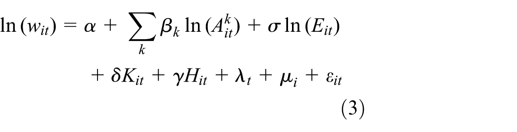
To investigate the spatial decay of urban agglomeration effects we separate the measure of employment accessibility into a series of contiguous travel time bands k, as shown in equation (3).
Finally, to examine the presence of nonlinearities in the productivity effects of urban agglomeration across MSA, we use a semiparametric partially linear model (e.g. Ruppert et al., 2003; Wood, 2006), where urban agglomeration enters the equation nonlinearly according to a smooth function f estimated using penalised spline regression techniques and the other terms are defined as in the equations above. This is illustrated in equation (4).

There are important identification issues that need to be considered in the estimation of the models above, namely possible endogeneity of urban agglomeration due to omitted variable bias or unobserved heterogeneity, and reverse causality between urban agglomeration, human capital and labour productivity. Individual unobserved heterogeneity is generally addressed through the use of the random-effects (RE) and fixed-effects (FE) estimators. The RE estimator assumes that unobserved heterogeneity is not correlated with the observed covariates, which if false leads to inconsistent and biased parameter estimates. On the other hand, although the FE estimator allows for correlation between unobserved heterogeneity and the model covariates, it can result in a great loss of efficiency in the presence of highly persistent data, as is typically the case of spatial agglomeration. A more flexible approach is the correlated random-effects (CRE) estimator, which includes the mean of the covariates and allows testing the assumption of no correlation between unobserved heterogeneity and model covariates (Chamberlain, 1982; Mundlak, 1978). In the case of reverse causality, the concern is that more productive metropolitan areas may attract workers with higher education, thus further increasing urban agglomeration and educational attainment. The remedial strategy adopted in the literature is to use instrumental variable (IV) estimators. The most common instruments used in the agglomeration literature include long-lagged values of urban agglomeration (Ciccone and Hall, 1996; Combes et al., 2010; Rice et al., 2006) and geological and geographical instruments (Ciccone, 2002; Combes et al., 2010; Glaeser and Gottlieb, 2009; Rosenthal and Strange, 2008). Given the changes in MSA boundaries over time, it is difficult to construct an instrument for urban agglomeration based on deep time lags. Alternatively, we follow an approach similar to that of Fingleton (2003, 2006) and use a five-group method which ranks the endogenous variable into one of five quintiles according to its size and then defines the instrument as the rank order (i.e. quintiles). The rationale is that there is strong association between the rankings of urban agglomeration and urban agglomeration size, but there is no relation between the relative rankings and labour productivity other than through the value of urban agglomeration. To instrument human capital, we follow Moretti (2004a) who used a deep time lag for the presence of colleges and universities as created in the 19th century by The Land Grant Movement.
Data
The dataset consists of a balanced panel of the 50 largest MSAs in the United States with a population of at least 1 million. The time horizon of the study is limited by data availability for employment accessibility, which is available for 1990, 1995, 2001 and 2009. The data sources and variables used in the study are described in the following paragraphs.
Labour productivity
To represent labour productivity, we use data for average MSA wage per job, available from the Regional Economic Information System (REIS) of the Bureau of Economic Analysis (BEA). To calculate real average wage per job (w) we use the GDP deflator with base year for 1990.
Urban agglomeration: Employment density vs. employment accessibility
We consider two measures of urban agglomeration: employment density and employment accessibility. The former has been extensively used in the empirical literature and although it is generally preferred to simple measures of total population and employment, its main limitation is that it assumes a uniform distribution of people across space and it does not account for the role of the transport network on actual spatial proximity, which our measure of employment accessibility does. Employment accessibility is defined in equation (5) as the number of jobs a representative traveller can reach within a certain travel time threshold.

where,
• Dt = metropolitan area employment density at year t
• k = time band (in minutes)
• Vn,t = average network speed in km/h at year t
• Ct = average circuity at year t
Because we do not have microdata on speeds by link going back to 1990 (this is only widely available, for a fee, in recent years with the advent of GPS), average metropolitan speeds estimated from a variety of data by the Texas A&M Transportation Institute (TTI) in their Urban Mobility Report are used, comprising a weighted average of arterial and freeway speeds. Similarly, micro level employment (at the block level) is not available consistently before the Census LEHD datasets became available in 2003, so urban employment density is used. The average circuity is the ratio of the shortest path network distance to the Euclidean distance and has been computed in a separate study (Levinson and El-Geneidy, 2009). For more details about the calculation of employment accessibility see Levinson (2012).
The representative traveller experiences uniform metropolitan average employment density, metropolitan average network speed and circuities that vary by trip length. All variables change with year. The maximum distance (or time) travelled is constrained so that once the representative traveller reaches a band where s/he passes all metropolitan jobs, the accessibility is capped (i.e. the region does not go on infinitely, only so long as all jobs at average density are available).
The distribution of employment across the travel time bands between 10 and 90 minutes indicates that 15% of employment is accessible within the first 10 minutes, and this value increases to 54% for 20 minutes, 83% for 30 minutes, 94% for 40 minutes, 98% for 50 minutes and 99% for 60 minutes. As a result, on average, the full majority of employment is accessible within one hour’s travel time. Unfortunately, our measure of employment accessibility is solely based on the road transport network and hence does not account for the role of public transport, which is likely to be important in the largest urban areas. 2 The average mode share for work trips in the US for 2013 is 76.4% drive alone and 9.4% carpool, compared with 73.2% and 13.4% in 1990. It is lower in the largest metro areas, but even there automobile dominates (e.g. 59% for metropolitan New York, 73.6% for San Francisco) (McKenzie, 2015).
Economic structure
To account for differences in the economic structure of metropolitan areas that might also affect their wage composition we use a measure of relative economic specialisation based on the Krugman Specialisation Index (K) (Krugman, 1991).

where
Human capital
Human capital (E) is measured by the percentage of population aged 25 years and over holding a bachelor’s degree or higher. Data for educational attainment were obtained from the decennial Census (for 1990 and 2000) and from the American Community Survey (ACS) for 2009. Using 2000 data for 2001, we had data for 1990, 2001 and 2009. Unfortunately, data were not available for 1995 as the ACS was conducted for the first time in 1996 in four counties only. To avoid losing a quarter of the observations we interpolated the 1995 educational data using a compound annual growth rate between 1990 and 2000.
Cost of living and local amenities
Wages are generally higher in larger urban areas, even after correcting for differences in housing costs. Spatial variation in real wages can reflect differences in the availability and quality of urban amenities. To account for differences in the cost of living we use the Federal Housing Finance Agency (FHFA) house price index (H) for each MSA. We adjust the original index to be centred on the mean value of the index for our sample of metropolitan areas and to have 1990 as the baseline year. Lower real wages might be more acceptable where climate is pleasurable, while areas with hostile climate might have to offer higher real wages to attract people (Glaeser et al., 2001). To account for this we use controls for the climate region a given MSA belongs to based on the nine climate regions identified by the National Climatic Data Center (Karl and Koss, 1984).
Table 1 provides basic descriptive statistics for the variables, while Figure 1 shows scatter plots for the relationship between metropolitan area average wage and the measures of urban agglomeration (i.e. employment density and employment accessibility) and human capital. There is a strong positive correlation between average wages and employment density (0.60) and educational attainment (0.74), and a relatively less strong correlation for employment accessibility, especially within 20 minutes’ travel time (0.15). The latter might result from greater congestion effects in the core urban areas of metropolitan areas. The correlation between average wages and employment accessibility is very similar across the travel time bands for 30, 60 and 90 minutes − 0.45, 0.54 and 0.55, respectively. This is expected because the number of jobs accessible within 30 and 60 minutes’ travel time corresponds to approximately 83% and 99% of the MSA employment accessible within 90 minutes, respectively.
Descriptive statistics of variables.
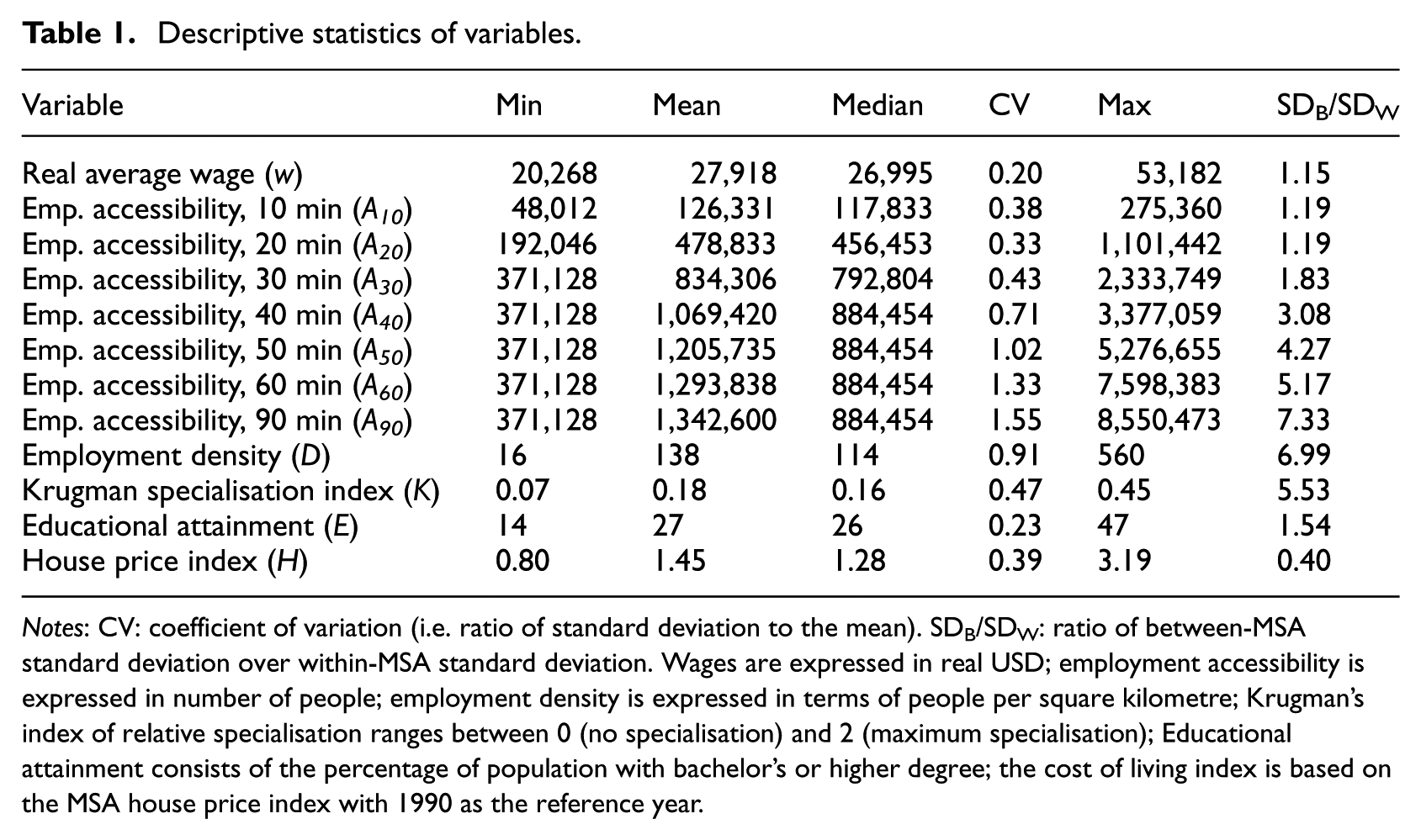
Notes: CV: coefficient of variation (i.e. ratio of standard deviation to the mean). SDB/SDW: ratio of between-MSA standard deviation over within-MSA standard deviation. Wages are expressed in real USD; employment accessibility is expressed in number of people; employment density is expressed in terms of people per square kilometre; Krugman’s index of relative specialisation ranges between 0 (no specialisation) and 2 (maximum specialisation); Educational attainment consists of the percentage of population with bachelor’s or higher degree; the cost of living index is based on the MSA house price index with 1990 as the reference year.
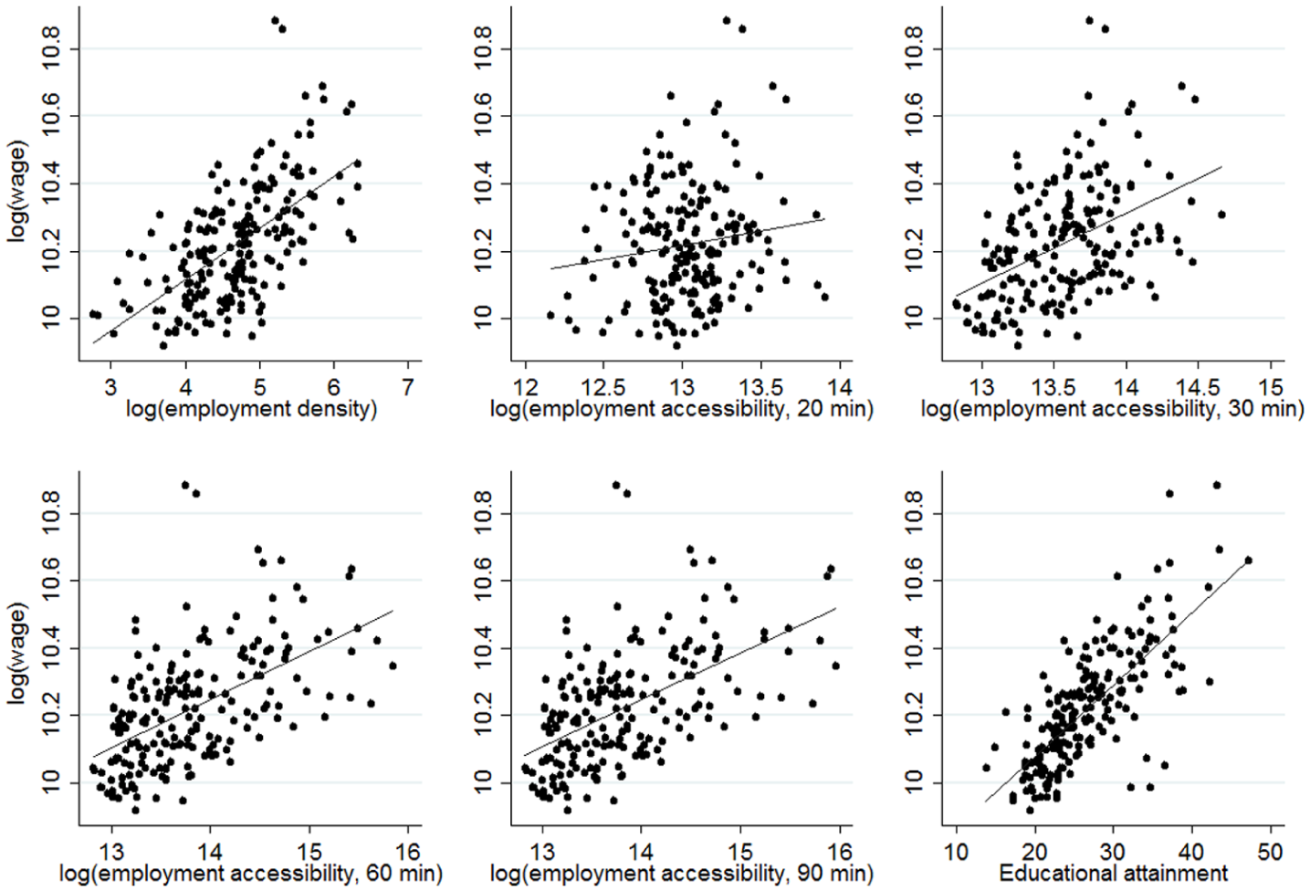
The relationship between real average wages, urban agglomeration and educational attainment.
Results and discussion
This section presents and discusses the main findings. The results obtained from the IV and non-IV models using RE, FE and CRE estimators are presented in Tables 2 to 4, respectively. Table 2 shows the models in which urban agglomeration is measured by employment density, while Table 3 reports the results for the models based on employment accessibility. Table 4 and Figure 2 refer to the models testing the spatial decay of the productivity gains from urban agglomeration across a set of successive travel time bands. The last part of the section discusses the analysis of nonlinearities in the relation between productivity and urban agglomeration (Figure 3).
Results of the wage models using employment density.
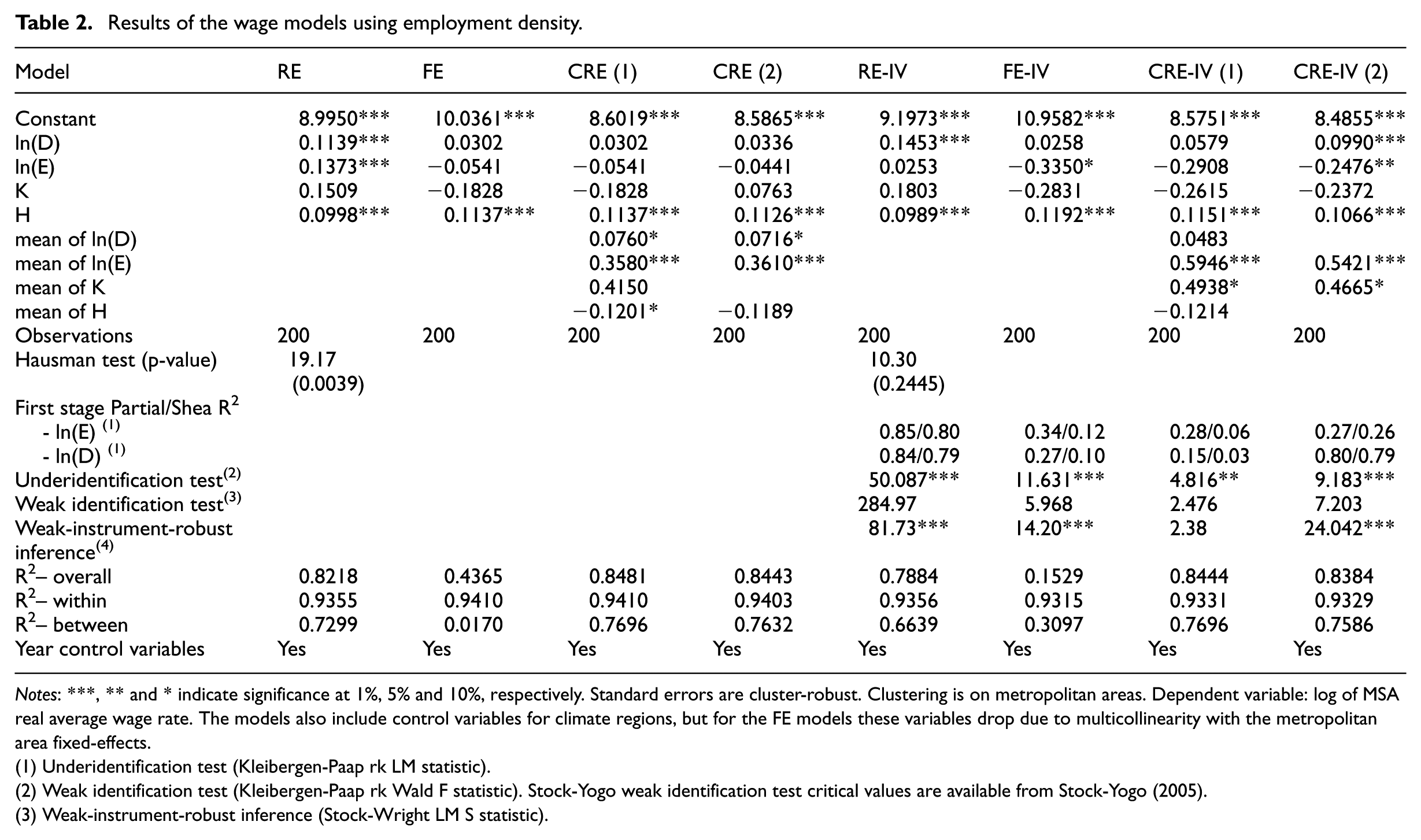
Notes: ***, ** and * indicate significance at 1%, 5% and 10%, respectively. Standard errors are cluster-robust. Clustering is on metropolitan areas. Dependent variable: log of MSA real average wage rate. The models also include control variables for climate regions, but for the FE models these variables drop due to multicollinearity with the metropolitan area fixed-effects.
Underidentification test (Kleibergen-Paap rk LM statistic).
Weak identification test (Kleibergen-Paap rk Wald F statistic). Stock-Yogo weak identification test critical values are available from Stock-Yogo (2005).
Weak-instrument-robust inference (Stock-Wright LM S statistic).
Results of the wage models using employment accessibility.

Notes: ***, ** and * indicate significance at 1%, 5% and 10%, respectively. Standard errors are cluster-robust. Clustering is on metropolitan areas. Dependent variable: log of MSA real average wage rate. The models also include control variables for climate regions, but for the FE models these variables drop due to multicollinearity with the metropolitan area fixed-effects.
Underidentification test (Kleibergen-Paap rk LM statistic).
Weak identification test (Kleibergen-Paap rk Wald F statistic). Stock-Yogo weak identification test critical values are available from Stock-Yogo (2005).
Weak-instrument-robust inference (Stock-Wright LM S statistic).
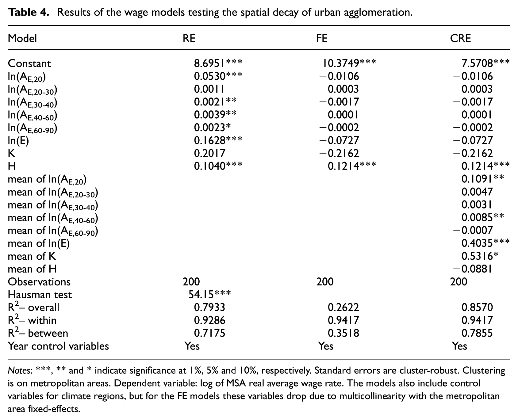
Results of the wage models testing the spatial decay of urban agglomeration.
Notes: ***, ** and * indicate significance at 1%, 5% and 10%, respectively. Standard errors are cluster-robust. Clustering is on metropolitan areas. Dependent variable: log of MSA real average wage rate. The models also include control variables for climate regions, but for the FE models these variables drop due to multicollinearity with the metropolitan area fixed-effects.
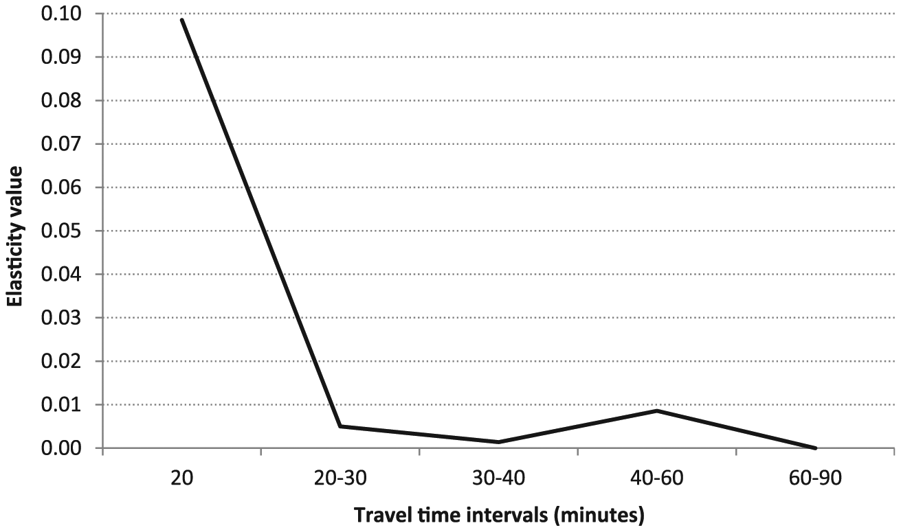
Spatial decay of urban agglomeration effects based on employment accessibility.

Nonparametric fit of the relation between metropolitan area wages (vertical axis) and urban agglomeration (horizontal axis): employment density (top) and employment accessibility (bottom).
Productivity gains from urban agglomeration
We first discuss the results in Table 2. Overall the models have good explanatory power with generally high coefficients of determination (R2). The first four columns of the table refer to the non-IV models, while the last four columns refer to the IV models. 3 The discussion focuses on the preferred models selected using appropriate tests for model comparison. 4 The elasticity of wage with respect to employment density obtained from the preferred model CRE (2), which includes correlated random-effects for employment density, educational attainment and housing costs index, is 0.072; this indicates that increasing employment density by 10% increases wages, all else equal, by 0.72%. Correcting for reverse causality appears to have a minor impact on the effect of urban agglomeration, which increases from 0.072 to 0.099 (CRE-IV (2)).
The models in Table 3 are based on the 60 minutes’ travel time band accounting for the large majority of metropolitan employment. The results obtained from the preferred model CRE (2), which includes correlated random-effects for employment density, educational attainment and relative industrial specialisation, are in line with those obtained in Table 2 for employment density. 5 Raising employment accessibility by 10% is associated with an increase in wages of 0.96%. Similarly, correcting for reverse causality does not seem to change the elasticity estimate for employment accessibility, which is equal to 0.095 (CRE-IV (2)).
The findings reported above for the effect of urban agglomeration on average labour productivity are consistent between the two measures used and suggest that incorporating information on network speeds does not seem to affect the results much, which seem to be mainly driven by density effects. This may be partly due to the fact that employment accessibility is based on average metropolitan speeds, which do not vary as much as density. Our preferred estimates indicate an elasticity value between 0.07 and 0.10. Corroborating other studies (e.g. Ciccone, 2002; Ciccone and Hall, 1996), we find that correcting for reverse causality does not much affect the magnitude of the estimates.
Overall, the magnitudes of the urban agglomeration elasticity estimates appear to be slightly higher than those obtained in previous studies using aggregate regional level data for the United States; however, these differences are considered reasonable because our analysis is focused on the 50 largest metropolitan areas for which we expect to observe stronger returns to urban agglomeration. Ciccone and Hall (1996), using data for 1988, found that doubling county employment density increased productivity by about 6%. More recent evidence for the United States based on metropolitan area data suggests that the urban agglomeration elasticity ranges between 5 and 8%. Glaeser et al. (2001) and Glaeser and Resseger (2010) found that doubling metropolitan area population leads to an increase in average labour productivity of about 5% for 1980 and 8% in 1990 and 2001.
Table 4 presents the results for the spatial decay models using a series of consecutive travel time bands between 20 and 90 minutes. The CRE model is selected as the preferred model because it provides consistent and more efficient parameter estimates than the FE model. 6 The results suggest that the spatial scope of the productivity effects of agglomeration can extend up to 60 minutes’ driving time, although the bulk of the effects occur within the first 20 minutes. The magnitude of the effect reduces dramatically for the following travel time bands and tends to be statistically insignificant (with the exception of the travel time band between 40 and 60 minutes). This pattern of a steep spatial decay is illustrated in Figure 2, and supports the view of very localised benefits from spatial agglomeration while at the same time reaching as far as, but not necessarily in a continuous way, the boundaries of labour market areas.
In a report describing commuting patterns in the United States, McKenzie and Rapino (2011) show that the average one-way travel time to work was about 22 minutes in 1990 and 25 minutes in 2000, and remained at 25 minutes in 2009. This commuting pattern is in line with stronger urban agglomeration effects within 20 and 30 minutes of travel time, as found in our analysis. In addition, similar findings of a steep spatial decay of urban agglomeration effects were also obtained from wage models based on driving time accessibility measures for Great Britain (Rice et al., 2006) and physical distance accessibility measures for the US (Rosenthal and Strange, 2008), Italy (Di Addario and Patacchini, 2008) and the UK (Melo and Graham, 2009).
Finally, we consider the results obtained from the semiparametric analysis. This approach does not make any assumptions on the functional form of the relationship between productivity and urban agglomeration, and allows the shape of the curve to be drawn as much as possible from the data. This provides a good way of investigating if there are ‘size’ thresholds above which the benefits from additional agglomeration become disproportionally greater or smaller.
The sample used consists of the 50 largest metropolitan areas, and hence contains considerably less variation than a full sample of large, medium and small metropolitan areas. As a result, the findings should be considered in the context of large and very large urban areas. Nonetheless, there is still more than an order of magnitude (about 20-fold) variation in the size of the metropolitan areas in the sample. Taking the year 2009 as reference, the latest year in our dataset, we observe that 60% of the sample consists of metropolitan areas with a population between 1–2.5 million, 22% of the sample consists of areas with a population between 2.5–5 million, 14% of the sample consists of areas with a population between 5–9 million and only 4% of the sample consists of metropolitan areas with a population of 10 million or more.
Figure 3 illustrates the nonparametric fit of the metropolitan area average real wage and urban agglomeration, where urban agglomeration is measured by employment density (top panel) and employment accessibility (bottom panel). 7 The vertical axis shows the value of the nonparametric fit of the dependent variable and the horizontal axis shows the values of urban agglomeration. The shaded area corresponds to the interval determined by the two standard error lines above and below the estimate of the smooth curve. The shape of the curves does not reveal significant nonlinear effects, and indeed we cannot reject the test with null hypothesis that the nonparametric fit can be approximated by a parametric linear fit. 8 This indicates that it is overall reasonable to assume a linear relation between spatial agglomeration and productivity for urban areas with and above 1 million people, and that there are no significant ‘threshold effects’ across urban areas of these sizes. It also suggests that there is no ‘wider economic benefits’ or ‘agglomeration economies’ rationale for allocating disproportionally more public investment to the top larger metropolitan areas compared to other large and very large metropolitan areas.
The main difference between the two curves is the downward sloping trend for the metropolitan areas with the highest employment density, although this effect appears to be statistically insignificant. One partial explanation for this difference might be the inability to disentangle congestion from high densities. It has been shown elsewhere (Levinson, 2012) that there is often a trade-off between high densities and lower mobility resulting from increased travel times and congestion. However, accessibility levels may vary between high density urban areas as a result of differences in the spatial organisation (e.g. urban form) and the planning and quality of transport systems. This implies that transport-based measures of urban agglomeration such as our measure of employment accessibility may be better able to disentangle, even if only partially, the effect of increased congestion from that of increased density.
Human capital, economic structure and cost of living
As expected, educational attainment helps explain spatial differences in average wages across metropolitan areas. The effect is consistent across the models reported in Tables 2 to 4 and suggests that increasing educational attainment by 10% is associated with an increase in wages between 3–4%. As for economic structure, our analysis based on the Krugman index of relative specialisation could not identify any conclusive effect for its relationship with average metropolitan area wage. Future analysis on this topic could attempt to combine this indicator with a measure of the type of industrial specialisation as a way to further explore issues relating to industry mix. However, for the purpose of our analysis we were mainly interested in separating the effects of urban clustering from those of industrial clustering. The models also show that an increase of 1 point in the house price index is associated with a less than proportional increase in average wage.
Conclusions
This paper contributes to ongoing research on the productivity gains from urban agglomeration by empirically examining the spatial decay and nonlinearity of these effects using a new transport-based measure of urban agglomeration and semiparametric techniques. To the best of our knowledge this paper provides the first attempt to test for potential nonlinearities in the productivity gains from urban agglomeration for the United States using semiparametric techniques.
The findings suggest that the productivity-agglomeration effects obtained for our sample of MSA are generally consistent between the two measures of urban agglomeration used – employment density and road transport-based employment accessibility. This suggests that, in the context of our study, metropolitan areas’ densities seem to have a stronger role than road network speeds in the realisation of urban agglomeration externalities. The second main finding is that the large majority of the productivity-agglomeration effects occur within the first 20 minutes, which is in agreement with previous evidence on very localised benefits, while remaining significant but small at wider distances encompassing the boundaries of labour markets. Furthermore, the analysis suggests that the returns to additional spatial agglomeration for our sample of large and very large metropolitan areas appear to be constant; however, this result should not be generalised to the more heterogeneous population of metropolitan areas in the United States, for which there may be significant ‘threshold effects’.
Some policy implications can be drawn from our findings. Evidence of a localised nature of spatial agglomeration effects suggests that within metropolitan areas immediate access (within 20 minutes) to jobs is very important for productivity, which in turn highlights the importance of investing in efficient transport networks. In addition, the lack of evidence in favour of nonlinearities in the relationship between productivity and urban agglomeration suggests there is no economic argument for allocating disproportionally more public money, to improve density and (road) transport accessibility, to the larger regions in our sample of metropolitan areas with 1 million people or more.
Footnotes
Funding
This research received no specific grant from any funding agency in the public, commercial, or not-for-profit sectors.