
Abstract
This paper examines the relationships between county-level urbanisation, natural amenities and subjective well-being (SWB) in the US. SWB is measured using individual-level data from the Behavioral Risk Factor Surveillance System (BRFSS) which asks respondents to rate their overall life satisfaction. Using individual-level SWB data allows us to control for several important individual characteristics. The results suggest that urbanisation lowers SWB, with relatively large negative coefficients for residents in dense counties and large metropolitan areas. Natural amenities also affect SWB, with warmer winters having a significant positive relationship with self-reported life-satisfaction. Implications for researchers and policymakers are discussed.
Introduction
Happiness, life-satisfaction and well-being are important topics for individuals, policymakers and researchers, but there is still much that is unknown about these outcomes. Researchers interested in these topics often analyse data from surveys that ask individuals to report their subjective assessment of their own life-satisfaction, which is commonly referred to as subjective well-being (SWB). 1 A number of factors have been found to affect SWB, typically in expected directions. Reviews of the SWB literature are provided by Diener and Biswas-Diener (2002), Dolan et al. (2008) and MacKerron (2012).
Many researchers have hypothesised that individual well-being may be considerably affected by the physical, social and economic environment in which the individuals are situated. There is some support for this contention using data from countries around the world, but empirical research on geographic differences in subjective well-being across the US has been relatively scarce largely because of limited data. However, the Behavioral Risk Factor Surveillance System (BRFSS) began asking individuals to report their subjective well-being in 2005 and provides large samples sizes and geographic identifiers needed to reliably assess spatial differences in SWB across the US. Oswald and Wu (2010, 2011) and Glaeser et al. (2014a) have examined these data and documented that there are indeed differences in subjective well-being across states and metropolitan areas in the US, but there are still numerous issues in need of further exploration to increase our understanding of these differences.
This paper uses the 2005–2010 BRFSS to examine the relationships between county urbanisation, natural amenities and individual subjective well-being. Specifically, we measure county urbanisation in two separate ways, first based on a single continuous variable for population density and then based on a set of categories for metropolitan status and size. Natural amenities examined relate to weather, topography and proximity to water. We use individual-level data and therefore can also control for individual characteristics that could confound analyses using aggregate data. Our approach to measuring urbanisation combined with using individual level US data is novel in the SWB literature. Additionally, we are the first researchers to our knowledge to examine relationships between county-level natural amenities and SWB across the US.
Previewing the results, we find suggestive evidence that urbanisation lowers individual subjective well-being, especially for residents of dense counties and large metropolitan areas. We also find that areas with warmer Januaries have happier residents. These results have important implications for researchers and policymakers interested in improving well-being. Specifically, policies that increase urbanisation may decrease individual well-being. Furthermore, Lucas (2014) suggests that local subjective well-being levels predict future population growth. Planners and forecasters need to be aware of these differences in well-being across areas.
Conceptual framework and literature review
General considerations
Various locational characteristics have been posited to affect various notions of individual well-being. For example, an individual’s well-being in a given location could be affected by local labour market conditions, prices of local goods and services and the presence and quality of location-specific amenities and disamenities. In particular, individual well-being is thought to be increasing in the local wage level and amenities and decreasing in the level of housing prices and disamenities. However, there is a pervasive belief that individuals’ ability to migrate from one place to another should greatly reduce the extent of well-being differences across places (Glaeser et al., 2014a, 2014b; Oswald and Wu, 2011; Roback, 1982; Winters, 2009).
Much research in regional and urban studies posits that areas should achieve a spatial equilibrium, at least in the long run. 2 The spatial equilibrium hypothesis suggests that freely mobile individuals with identical skills and preferences should receive equal utility across all areas. If not, some individuals will have an incentive to move. More specifically, individuals will move from areas offering low levels of utility to areas offering higher utility (Glaeser et al., 2014b). As they relocate, they alter local markets for both labour and housing by increasing the supply of labour and the demand for housing in their new locations and reducing the supply of labour and demand for housing in their old locations. In unconstrained competitive markets, prices will adjust to achieve equilibrium. As workers move from low utility to high utility areas, wages and housing prices will adjust to push markets toward spatial equilibrium. Specifically, population growth will bid up housing prices and apply downward pressure on wages, so that the initial utility gap between the areas diminishes.
However, researchers have documented that there are indeed spatial differences in self-reported life-satisfaction, even controlling for individual differences such as age, race, ethnicity and education (Glaeser et al., 2014a, 2014b; Okulicz-Kozaryn, 2015; Oswald and Wu, 2010, 2011). A natural next question then becomes what is causing these spatial differentials in SWB? Do they represent short-term differences from transitory shocks that require movement from one equilibrium to another? Do they simply capture unobserved differences in skills, preferences, expectations or reporting scales across workers in different areas? Glaeser et al. (2014a, 2014b) suggest that spatial differentials in SWB may result because individual utility depends on more than just what one considers when providing a subjective response to typical life-satisfaction questions. Specifically, individuals may be willing to trade off SWB for other things like consumption, leisure, social status and accomplishments; these likely affect SWB but might also affect individual utility independently of SWB. Furthermore, individuals may prefer to take actions that help achieve various long-term desires and goals yet that make them less happy at the time of the survey.
Another possible explanation for spatial SWB differentials is that there may be barriers to migration that prevent the spatial arbitrage process from fully equating happiness across areas. The US has historically experienced relatively high internal migration rates compared to other developed countries, but internal migration has fallen in the US in recent years perhaps because of decreased responsiveness to spatially asymmetric demand shocks (Partridge et al., 2012). Furthermore, Krupka (2009) suggests that individuals may make location-specific human capital investments that increase the benefits from living near familiar amenities and deter relocation to highly dissimilar areas. 3 Additionally, some people likely develop special attachments to places where they grew up or had other formative experiences; places may become part of their identity and they are reluctant to leave. Krupka and Donaldson (2013) suggest that heterogeneous moving costs combined with housing supply constraints may bias traditional hedonic estimates of amenity values. Location-specific preferences, heterogeneous moving costs and other frictions constraining mobility imply that infra-marginal residents in one city may achieve different utility levels than infra-marginal residents in another city. Thus, spatial arbitrage in housing and labour markets may equate utility across areas for marginal migrants without doing so for infra-marginal migrants. 4
While life-satisfaction responses may not equal utility, an individual’s life-satisfaction at a point in time certainly has an important effect on utility and is an important outcome for researchers to study. The current paper examines the relationships between local urbanisation and natural amenities and individuals’ self-reported life satisfaction. That these factors might affect well-being is not new, but the approach taken in this paper is novel in many ways and aims to provide additional insights to the existing literature.
Urbanisation might affect individual well-being in numerous ways, both positively and negatively (Easterlin et al., 2011; Okulicz-Kozaryn, 2015). Positive effects of urbanisation on well-being might result from agglomeration economies and increased variety and quality of consumption opportunities. Agglomeration economies due to thick labour markets, intermediate input sharing and knowledge spillovers are thought to increase worker productivity and wages in larger and denser areas (Puga, 2010), which could increase life-satisfaction, ceteris paribus. Big cities may also offer better and more diverse consumption opportunities for numerous goods such as museums, theatres, music, professional sports, public transit, heath care and specialised restaurants (Albouy, 2008; Berry and Waldfogel, 2010; Borck, 2007; Glaeser et al., 2001). However, urbanisation also likely increases living costs, congestion, pollution, traffic and crime and reduces public greenspace, all of which can decrease life-satisfaction (Ambrey and Fleming, 2014; Berry and Okulicz-Kozaryn, 2011; Navarro-Azorín, and Artal-Tur, 2015; Sander, 2011; Smyth et al., 2008; Steiner et al., 2015; Stutzer and Frey, 2008). Increased urbanisation may also create a perceived need for urban planners to zone segregated uses and discourage mixed-use neighborhoods that Jane Jacobs (1961) viewed as critical for the well-being of cities and the people in them. Furthermore, urbanisation could affect social capital and alienation (McKenzie, 2008; Okulicz-Kozaryn, 2015), which can affect well-being (Helliwell, 2006; Helliwell et al., 2014). Similarly, urbanisation may reduce political capital and good governance and facilitate corruption and rent-seeking that lower average life satisfaction (Abdallah et al., 2008; Brueckner and Neumark, 2014). The net effect of urbanisation on well-being is ambiguous and depends on individual preferences for the good and bad attributes that cities possess. The current paper does not try to empirically sort out the magnitudes of the various mechanisms by which urbanisation might affect life-satisfaction. Instead, we focus on the overall effect of urbanisation on SWB, which is fundamentally important on its own.
A natural amenity can be broadly thought of as any naturally-occurring locational attribute that makes a location more desirable. Areas with better natural amenities might be expected to increase individual well-being. More generally, researchers have suggested that amenities related to nicer weather have played a central role in regional population redistribution in the US, especially from the nation’s ‘Rustbelt’, i.e. the older industrial Great Lakes region, to the nation’s ‘Sunbelt’, i.e. warmer areas in the South and West regions (Partridge, 2010; Rappaport, 2007; Rickman and Rickman, 2011; Rickman and Wang, 2015). 5
Literature on spatial SWB differentials
Oswald and Wu (2010, 2011) use the BRFSS to show significant differences in SWB across states in the US even controlling for numerous individual characteristics. Oswald and Wu (2010) also show that these SWB differences are correlated with state quality-of-life rankings based on hedonic pricing of locational amenities. Specifically, Oswald and Wu (2010) find that states with better quality of life have higher subjective well-being, but they do not examine the relationships with specific amenities. Oswald and Wu (2010, 2011) state SWB differences appear to be at least somewhat related to climatic differences between the Sunbelt and Rustbelt regions, but they do not provide formal evidence on this.
Natural amenities have also been considered to affect life-satisfaction and well-being by other researchers for other areas. Climate variables, in particular, have received considerable attention in the subjective well-being literature (Brereton et al., 2008; Cuñado and Pérez de Gracia, 2013; Fischer and Van de Vliert 2011; Maddison and Rehdanz, 2011; Moro et al., 2008; Rehdanz and Maddison, 2005). The literature suggests that both very hot summers and very cold winters reduce life-satisfaction. 6 The value of ecosystems and land cover has also been shown to affect SWB (Abdallah et al., 2008; Vemuri and Costanza, 2006).
Glaeser et al. (2014a) show that there are meaningful differences in subjective well-being across metropolitan areas of the US. They show that persons in declining urban areas experience lower SWB, and this appears particularly true for those in the nation’s Rustbelt. Glaeser et al. (2014a) also report regression-adjusted mean SWB levels for selected metropolitan areas showing that the nation’s largest metropolitan area, the New York City MSA, had the lowest life-satisfaction level in the country. Other large MSAs like Los Angeles, Chicago, Boston, San Francisco and San Jose tended to perform poorly as well, though there were some exceptions including Washington DC. Glaeser et al. (2014a) do not systematically examine the effects of population density on SWB. They do briefly examine the association with log MSA population, but do not find a consistent relationship; they do not examine metro status and size categories such as used in this study. Their analysis also employs MSA-level measures instead of county-level ones.
The literature on spatial differences in subjective well-being across the US is relatively small, and we make several contributions relative to the previous literature. 7 Our approach to measuring urbanisation at the county-level combined with controlling for individual characteristics is novel in the literature. A few studies have examined the relationship between population density and subjective well-being (Berry and Okulicz-Kozaryn, 2011; Cramer et al., 2004; Florida et al., 2013; Moro et al., 2008), but the only previous study to do so using US county-level data (Lawless and Lucas, 2010) uses county averages and does not control for individual characteristics. Measuring density at the county-level rather than the MSA-level is important because MSAs typically include both densely populated central areas and low-density suburban areas. Using a single density measure for an entire MSA hides these large differences and may inaccurately describe the relationship between density and SWB. Controlling for individual characteristics like age and education is important to isolate effects due to locational factors. For example, more educated persons may sort into high amenity and high density areas and confound relationships based on area averages. We are also the first researchers to our knowledge to explicitly estimate regression coefficients for county-level natural amenities using individual subjective well-being data across the US.
Empirical approach
This paper combines individual-level data from the 2005–2010 BRFSS with county-level data on urbanisation and natural amenities. The dependent variable is a measure of subjective well-being from the BRFSS. During this time period, the BRFSS asked individuals ‘In general, how satisfied are you with your life?’ Respondents were to choose answers from the following categories: Very satisfied, Satisfied, Dissatisfied or Very dissatisfied. Our analysis codes the life satisfaction categories from one to four with one being Very dissatisfied and four being Very satisfied, so that our variable is increasing with life satisfaction. A few survey participants either refused or were unsure about how to respond to the life satisfaction question; persons with invalid responses are excluded from the analysis. The analytical sample is also restricted to persons aged 18–85 living in a county that is identifiable in the BRFSS excluding Alaska and Hawaii. The BRFSS identifies a total of 2361 counties across this period but does not identify small counties with very few observations because of confidentiality concerns. The natural amenity data discussed below are unavailable for Alaska and Hawaii, necessitating their exclusion.
We use ordinary least squares (OLS) regression 8 to estimate variants of the following equation:

The dependent variable,
Summary statistics.
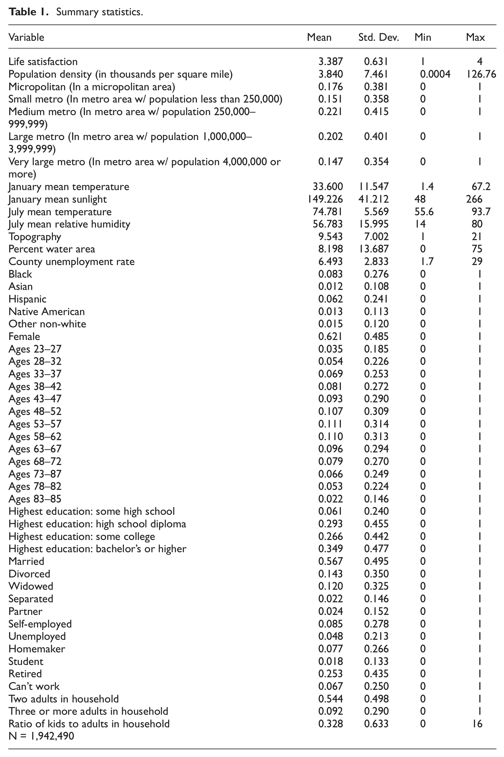
The interest in this study is on the relationships between urbanisation, natural amenities and subjective well-being. We measure urbanisation in two separate ways. We first measure urbanisation using a continuous variable based on the population density (in thousands of people per square mile) in the county in year 2000. The population density is measured based on the average density experienced by county residents and not the density experienced by the land (Glaeser and Kahn, 2004; Rappaport, 2008). Specifically, the density measure is computed by dividing the resident population for every census-defined block group by its land area and then computing a population-weighted average of block-group population density for each county. In results not shown, we also used the simpler raw density measure that is computed as county population divided by land area, which yielded qualitatively similar results with slightly different magnitudes; these results are available from the authors by request. County identifiers are the finest level of geographic detail available for SWB data across the US. To some extent, there could be additional advantages from an even finer level of geographic detail, for example in examining effects of proximity to endogenous amenities like parks, green spaces, museums, restaurants and shopping places. However, the gains from finer geographic detail are likely modest for examining overall effects of urbanisation and natural amenities, and county-level data still yield important insights. American metropolitan areas typically include multiple counties, with some large metros including dozens of counties. Furthermore, there is considerable variation in population density across counties, both across and within metropolitan areas.
Our second approach for measuring the extent of urbanisation is based on metropolitan area status and size. Specifically, we use year 2000 county population data and 2003 metropolitan and micropolitan area component classifications (both from the US Census Bureau) to assign each county to one of six categories. We classify metropolitan statistical areas (MSAs) as either small, medium, large or very large based on MSA population groupings of 0–249,999, 250,000–999,999, 1,000,000–3,999,999 and 4,000,000 or more, respectively. 10 We also divide non-metropolitan areas into micropolitan areas and non-urban areas. Non-urban areas are defined as areas that are part of neither a metropolitan nor micropolitan area. In the regression results below, non-urban counties are the excluded base group; coefficients for the metro status and size dummy variables are measured relative to this base group.
We examine six county-level natural amenity measures obtained from the United States Department of Agriculture (USDA) Economic Research Service (ERS) natural amenity database. These are described in McGranahan (1999) and include mean January temperature, mean January sunlight hours, mean July temperature, mean July relative humidity, topography (measured on a scale of 1–21 with higher values indicating a more mountainous land surface) and the percentage of total county area covered by water. Having a warmer and sunnier January is expected to increase life-satisfaction, while having a hotter and more humid July is expected to reduce life-satisfaction. The expected effect of topography is somewhat ambiguous; more mountainous topography may provide greater consumption amenities but make production more difficult and reduce employment outcomes. Water coverage is expected to provide greater recreational opportunities and increase life-satisfaction.
The later years of our data correspond to the Great Recession of 2007–2009 and the ensuing slow recovery. Year dummies will capture aggregate differences over time, but the economic downturn was more severe in some areas than others. Therefore, we also examine the robustness of our results to including the county annual unemployment rate computed by the US Bureau of Labor Statistics (BLS) in its Local Area Unemployment System (LAUS). Living in a stronger local labour market with lower unemployment rates is expected to increase well-being. Empirical evidence routinely finds that being unemployed reduces individual subjective well-being (e.g. Clark and Oswald, 1994; Oswald and Wu, 2011; Winkelmann and Winkelmann, 1998), but there is also evidence that the local unemployment rate in an area reduces the well-being of its residents, even among those who are currently employed (Helliwell and Huang, 2014). This latter finding could be because of increased risk of becoming unemployed or increased perception of unemployment risk.
Empirical results
We estimate the SWB equation for several regression specifications that include different sets of control variables in order to examine the sensitivity of the results. All regressions include month and year dummies and cluster standard errors by county.
Results for urbanisation measures
Table 2 presents the regression results for the urbanisation variables. We report results for the two measurement approaches in panels A and B. Results for the population density variable are reported in panel A, and results for the metropolitan area status and size dummies are reported in panel B. Each panel includes regression results for four specifications with differing variables included. Columns 1–3 include only one of the two approaches to measuring urbanisation, and column 4 includes both the population density and the metro status and size dummies jointly. Column 1 includes the urbanisation measure(s) but excludes all other variables except for month and year dummies. Column 2 adds the individual controls. Column 3 adds the county unemployment rate and the natural amenity variables as controls (results for natural amenities are reported separately in Table 3). Column 4 includes both sets of urbanisation measures along with all other variables in previous columns.
Regression results for urbanisation variables on life-satisfaction.
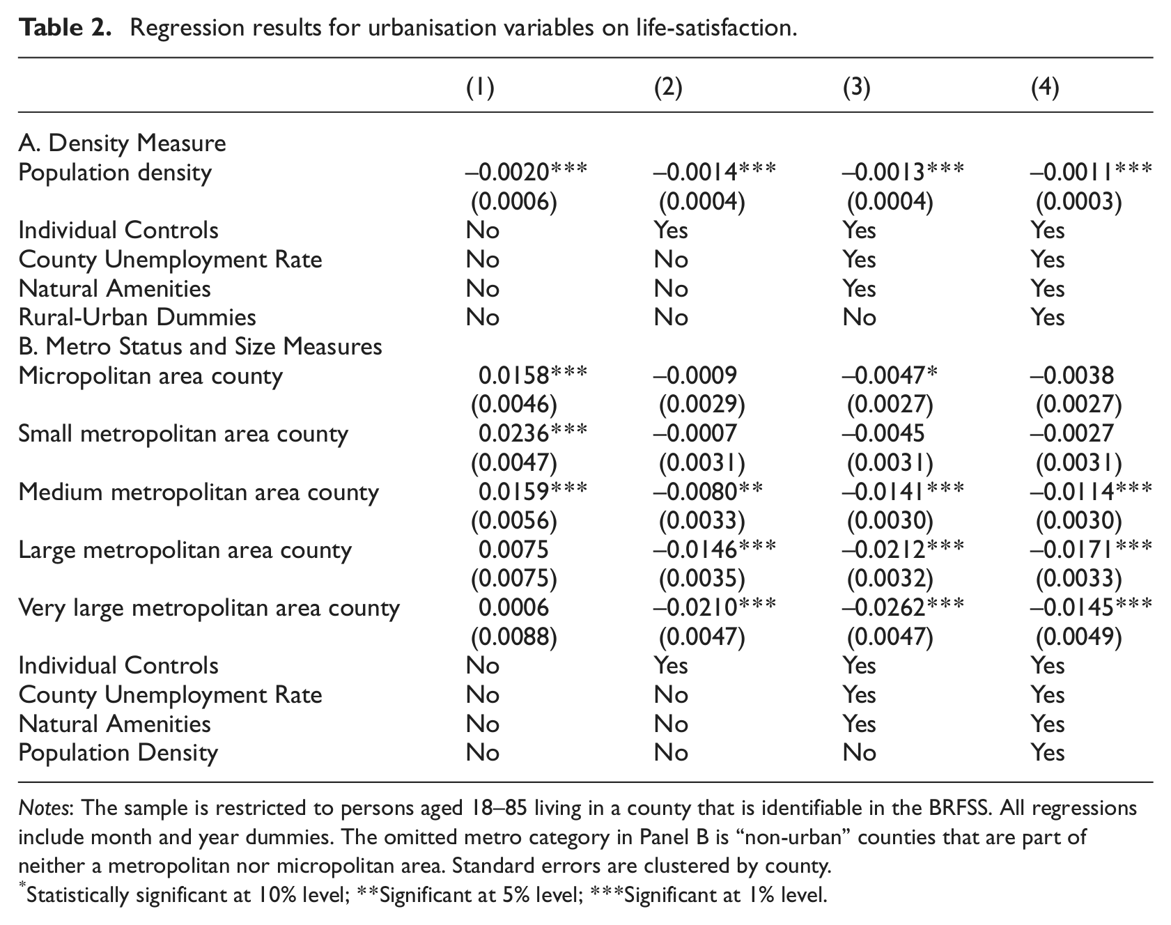
Notes: The sample is restricted to persons aged 18–85 living in a county that is identifiable in the BRFSS. All regressions include month and year dummies. The omitted metro category in Panel B is “non-urban” counties that are part of neither a metropolitan nor micropolitan area. Standard errors are clustered by county.
Statistically significant at 10% level; **Significant at 5% level; ***Significant at 1% level.
Regression results for natural amenities on life-satisfaction.
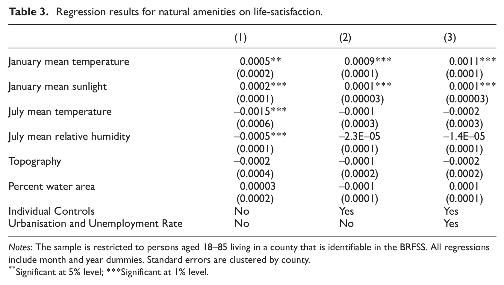
Notes: The sample is restricted to persons aged 18–85 living in a county that is identifiable in the BRFSS. All regressions include month and year dummies. Standard errors are clustered by county.
Significant at 5% level; ***Significant at 1% level.
The results in Panel A suggest that urbanisation as measured by county population density has a negative relationship with an individual’s subjective well-being. The coefficient is negative and statistically significant in all four columns. Interestingly, the coefficient does fall when individual controls are included, e.g. the coefficient falls from −0.0020 in column 1 to −0.0014 in column 2. This suggests that studies using aggregate data that do not control for individual characteristics may produce inaccurate results because of differences in individuals across areas. The specification in column 3 that also includes amenities and the unemployment rate yields a coefficient for population density of −0.0013. Adding the metro status and size dummies lowers the population density coefficient to −0.0011, but these are both measures of urbanisation, so column 4 partials out some of the urbanisation effect. Still, it is quite notable that the negative coefficient for density on SWB largely remains when controlling for city size.
Panel B reports results for the metro status and size dummies; the omitted base group is non-urban counties. With no controls in column 1, it appears that the relationship between urban utility and urban size has an inverted U-shape. Specifically, the highest well-being occurs in micropolitan areas (0.0158), small metro areas (0.0236) and medium metro areas (0.0159); large and very large metros are not statistically different from non-urban areas. However, controlling for individual characteristics in column 2 generates coefficients that are largely decreasing in urban size. Micropolitan areas and small metropolitan areas have small negative coefficients that make them statistically indistinguishable from non-urban areas. The coefficients are significantly negative for medium metros (−0.0080), large metros (−0.0146) and very large metros (−0.0210). Controlling for the county unemployment rate and natural amenities increases the magnitude of the metro status and size coefficients, and the micropolitan dummy is now significant with a coefficient of −0.0047; the coefficients for medium, large and very large metros are −0.0141, −0.0212 and −0.0262, respectively. Adding the county population density in column 4 reduces the metro status and size coefficients, and the micropolitan dummy is no longer statistically significant. The coefficients for medium, large and very large metro areas are still statistically significant but are reduced in magnitude to −0.0114, −0.0171 and −0.0145, respectively. The decrease is largest for very large metro areas suggesting that the negative coefficient for very large cities on SWB in column 3 is largely attributable to the negative relationship between density and SWB. Of course, the results in column 4 should be interpreted with some caution since we are including two competing measures of urbanisation.
Collectively, the results in Table 2 suggest that both population density and metropolitan area size significantly reduce individual life-satisfaction. There is considerable disagreement in the previous literature as to how cities affect the well-being of those living in them (Albouy, 2008; Glaeser et al., 2014a, 2014b; Sander, 2011). Cities certainly possess a number of both positive and negative attributes, but the empirical results in Table 2 suggest that living in dense and heavily-populated areas has an overall negative relationship with an individual’s subjective assessment of their own well-being. 11 We do not explore the specific attributes of cities that are driving this overall negative relationship, but this is an issue worthy of future exploration.
The negative relationship between urbanisation and SWB also raises the question of why so many people live in large and densely populated areas. One possibility is that SWB is a component of utility that is partially substitutable with other factors as suggested by Glaeser et al. (2014a, 2014b). If so, people may live in large and dense cities because doing so allows for greater wealth accumulation, human capital accumulation, social status and accomplishments that both affects SWB and is substitutable with it. This is in contrast to arguments that people live in large and dense cities because of greater consumption opportunities and quality of life. Alternatively, people have incomplete information about the actual happiness they would experience in different locations and may form upwardly biased expectations about their happiness in big cities that causes them to move to big cities (Okulicz-Kozaryn, 2015). Once there, they may make location-specific investments and develop attachments that make them reluctant to leave. Finally, big cities expose individuals to incredible consumption possibilities that a modest income cannot afford. Living in a big city may raise aspirations for income and consumption that are not attainable for most people, increasing their dissatisfaction. And the big city exposure may stick with people even after leaving, so that they cannot reduce their aspirations and increase their SWB by leaving. Many big city residents might have ultimately been happier if they were never exposed to big cities, but conditional on being exposed to a big city, moving may not make them happier.
Results for natural amenities
The regression results for natural amenities are reported in Table 3. Column 1 includes the six natural amenity variables but excludes all other variables except for month and year dummies. Column 2 adds the individual controls. Column 3 adds the county unemployment rate and all of the urbanisation measures as controls.
The coefficient estimates for the natural amenity variables do vary somewhat across specifications, but there are some commonalities as well. The coefficients for January temperature and January sunlight conform to expectations for all specifications, that is, they are positive and statistically significant, suggesting that warmer and sunnier Januaries increase life-satisfaction. This is consistent with previous literature showing that people have been moving to areas with nicer weather (Partridge, 2010; Rappaport, 2007; Rickman and Rickman, 2011; Rickman and Wang, 2015). Interestingly, the coefficient estimate for January temperature in column 3 (0.0011) is twice as large as in column 1 (0.0005) with no controls. However, the coefficient for January sun decreases moving from column 1 (0.0002) to columns 2 and 3 (0.0001 for both).
The coefficient for July temperature is statistically significantly negative in columns 1 as expected, but it is not statistically significant in columns 2 or 3. The lack of robustness prevents one from drawing strong conclusions about the effects of July heat on life-satisfaction. Similarly, July relative humidity is significantly negative in column 1 (–0.0005), but the coefficient decreases in magnitude and becomes statistically insignificant in columns 2 and 3. 12 Topography has a negative coefficient in all specifications but is never statistically significant, preventing us from making strong conclusions. The percent of water area is also statistically insignificant in all specifications.
Further sensitivity analysis
We next further consider how sensitive the results are to alternative specifications and samples. Table 4 presents some additional results for both urbanisation measures and natural amenities. Column 1 reproduces results for the ‘base specification’ with all of the variables included thus far, including both sets of urbanisation measures simultaneously; this corresponds to column 4 of Table 2 and column 3 of Table 3.
Results for alternative specifications.
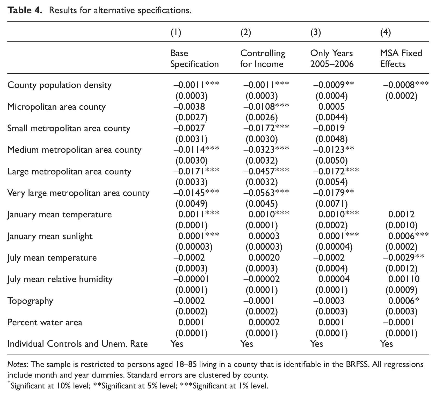
Notes: The sample is restricted to persons aged 18–85 living in a county that is identifiable in the BRFSS. All regressions include month and year dummies. Standard errors are clustered by county.
Significant at 10% level; **Significant at 5% level; ***Significant at 1% level.
Column 2 of Table 4 reports results that control for individual income using interval-coded survey responses in the BRFSS. It is certainly possible that higher ability (and hence higher income) individuals may differentially sort into areas based on the extent of urbanisation and natural amenities. However, we also recognise that higher incomes are one of the main benefits of urbanisation, and controlling for income hinders our ability to interpret the coefficients on our urbanisation measures as reporting overall effects. Examining the results in column 2, we see that the population density coefficient is still significant and unchanged in magnitude (–0.0011). However, the metropolitan status and size dummy coefficients are significantly affected. The coefficients become more negative, and are strongly increasing in magnitude with metropolitan area population. For example, very large metro areas have a very large coefficient of −0.0563.
The January temperature coefficient is slightly reduced (from 0.0011 to 0.0010) by controlling for income but it is still statistically significant. However, the coefficient for January sunlight is reduced and becomes statistically insignificant. The lack of robustness for January sunlight hinders our ability to make strong inferences about its relationship with subjective well-being. The other natural amenities remain statistically insignificant.
The results are somewhat sensitive to controlling for income, but controlling for one of the main benefits of urbanisation may be inappropriate if we are not also controlling for the costs of urbanisation like higher cost of living, increased congestion, etc. Controlling for cost of living at the county level is complicated by lack of data on non-housing prices and differences in user costs between home-owners and renters (Winters, 2009, 2013), so we make no attempt to do so but this could be an area for future research. There are many possible urban amenities and disamenities and including all possible relevant characteristics is not feasible. Thus, our preferred approach in this paper is to focus on the overall effects of urbanisation and natural amenities on subjective well-being. As such, our preferred results do not control for income since doing so would partial out a major benefit of large dense cities. However, it is worth emphasising that controlling for income does not change the directional relationship between urbanisation and subjective well-being; it only intensifies the magnitudes of the negative coefficients for city size that we observe.
Column 3 of Table 4 examines the sensitivity to limiting the sample to years 2005–2006. The primary motivation for doing so is to recognise that the housing crash, economic recession and generally sluggish economy experienced during years 2007–2010 affected some areas more than others. Restricting to years 2005–2006 reduces the magnitude of the density coefficient to −0.0009, but it is still significant. The metro status and size coefficients are largely unchanged except that the coefficient for very large metropolitan areas increases in magnitude from −0.0145 to −0.0179. The January temperature coefficient of 0.0010 is again significant and the coefficient for January sun is unchanged from the base specification. The other natural amenities are again statistically insignificant.
Column 4 of Table 4 examines the sensitivity to including fixed effects for each metropolitan area (MSA). This regression only uses variation in density and natural amenities within metro areas. The metro status and size dummy coefficients are no longer estimable due to collinearity with the MSA fixed effects. Results show that county-level density still has a significant negative coefficient, though it is now reduced to −0.0008. Thus, density decreases life satisfaction even within metro areas. However, some of the observed negative effect of density in Table 2 is due to differences across metro areas. The January temperature coefficient of 0.0012 is very similar in magnitude to the baseline estimates, but it is now much less precisely estimated and not statistically significant at the 10 percent level. However, January mean temperature does not vary much within most metro areas, so the imprecision is not surprising and should not be interpreted as evidence inconsistent with the findings in the base specification. Interestingly though, including MSA fixed effects increases coefficient magnitudes for January sunlight and July temperature, which are now statistically significant in expected directions at 0.0006 and −0.0029, respectively. Topography is also now statistically significant at the 10 percent level with a coefficient of 0.0006.
Conclusion
Most individuals care about both their own well-being and the well-being of others. Researchers and policymakers are interested in how various factors affect individual well-being, in part because of interest in improving the well-being of others. However, there is still limited knowledge about what factors actually improve individual well-being. Locational factors have been hypothesised to affect well-being, but the previous literature offering empirical evidence is quite limited, especially for the US. This paper examines relationships between county-level measures of urbanisation and natural amenities and subjective well-being using individual-level data from the BRFSS.
We find evidence consistent with expectations that more extreme climate conditions reduce subjective well-being. Specifically, warmer winter months are consistently associated with increased life satisfaction, and there is some evidence suggesting that January sunlight increases life satisfaction and hotter summer months reduce life satisfaction. Mobile individuals are expected to seek out areas offering them the highest well-being, so these spatial differences in SWB by climate suggest that the long-term US population redistribution to areas with nicer weather, especially those with warmer winters, is likely to continue for the foreseeable future.
The primary contribution of this paper, however, relates to the relationship between urbanisation and SWB. Living in an urban area conveys a number of both costs and benefits. Results in this study suggest that large and densely populated urban areas are associated with reduced individual life-satisfaction. Negative coefficients on SWB are found for both county population density and metropolitan area size. The implications depend in part on how individuals’ responses to the SWB question relate to their overall well-being and utility. To the extent that utility and SWB are distinct, individuals may tolerate lower SWB in large and dense urban areas because of the additional sources of utility that doing so confers such as greater human capital accumulation and accomplishments that affect both present and future life-satisfaction. However, biased expectations, location-specific investments and raised aspirations may also be important.
The results in this study should also be of interest to policymakers. Public policies that constrain the population and density of urban areas may be able to improve individual life-satisfaction, for example, by reducing congestion, pollution and time spent commuting. However, there is still much that is unknown about the exact causes of the negative urbanisation coefficients, and these should be explored in future research to improve our understanding and help shape policy. Effective policy may be better directed towards treating the underlying causes of dissatisfaction rather than imposing crude constraints on urban size, density and growth. More generally, policy should continually aim to improve well-being by both better leveraging the benefits of cities such as higher productivity and human capital accumulation and minimising the costs that urbanisation creates.
Footnotes
Acknowledgements
The authors thank Randy Jackson, Mark Partridge, Conrad Puozaa, Jordan Rappaport, Dan Rickman, Heather Stephens, Michael Timberlake, anonymous reviewers and participants at the 2015 Southern Regional Science Association Meetings for helpful comments. Any errors are the responsibility of the authors. The main data used in this study are publicly available online from the BRFSS website. Stata code and supplementary data are available from the corresponding author by request.
Funding
This research received no specific grant from any funding agency in the public, commercial, or not-for-profit sectors.