
Abstract
In this paper we move away from a static view of neighbourhood inequality and investigate the dynamics of neighbourhood economic status, which ties together spatial income inequality at different moments in time. Using census data from three decades (1980–2010) in 294 metropolitan statistical areas, we use a statistical decomposition method to unpack the aggregate spatiotemporal income dynamic into its contributing components: stability, growth and polarisation, providing a new look at the economic fortunes of diverse neighbourhoods. We examine the relative strength of each component in driving the overall pattern, in addition to whether, how, and why these forces wax and wane across space and over time. Our results show that over the long run, growth is a dominant form of change across all metros, but there is a very clear decline in its prominence over time. Further, we find a growing positive relationship between the components of dispersion and growth, in a reversal of prior trends. Looking across metro areas, we find temporal heterogeneity has been driven by different socioeconomic factors over time (such as sectoral growth in certain decades), and that these relationships vary enormously with geography and time. Together these findings suggest a high level of temporal heterogeneity in neighbourhood income dynamics, a phenomenon which remains largely unexplored in the current literature. There is no universal law governing the changing economic status of neighbourhoods in the US over the last 40 years, and our work demonstrates the importance of considering shifting dynamics over multiple spatial and temporal scales.
Introduction
In 2018, the United Nations reported that
Increasing urbanisation is occurring alongside a return to historic levels of interpersonal income inequality (Piketty and Saez, 2003). Not all members of society have benefited equally from the extensive economic growth experienced over recent decades. Instead, the wealthiest parts of the income distribution have claimed the lion’s share of the growth. While these patterns have been well documented, what is unclear is if this form of distributional polarisation is being played out within expanding cities fuelling the urbanisation process. More specifically, we do not know if the growth of cities exacerbates the level of spatial inequality within cities, or if the aggregate growth of a city triggers new types of neighbourhood dynamics. The measure of such dynamics is similar to the income mobility measure in the individual income distribution literature that ties together income inequality at different moments in time. Reframing income mobility to the case of neighbourhood dynamics within a metropolitan context provides us with the opportunity to examine questions surrounding urbanisation and spatial polarisation.
In this paper, we examine the patterns of neighbourhood income dynamics across US metropolitan areas over the period 1980–2010. In doing so, we pose the following questions. First, we focus on the direction of neighbourhood income dynamics – have there been secular increases, decreases, or have these patterns been episodic? Second, what have been the roles of different components of neighbourhood income dynamics? As we discuss more fully below, a global indicator may mask different types of dynamics. Therefore, unpacking the contributions of these different types of dynamics is an important undertaking. Third, are these patterns spatially uniform, or is there spatial heterogeneity in neighbourhood dynamics across the US? If it is the latter, what are the underlying mechanisms?
This paper contributes to the literature on neighbourhood dynamics in the urban US in four ways. Firstly, we consider a large number of US metropolitan areas, including not only the largest cities, but also those in the middle and lower tail of the city size distribution; this sample yields over 54,000 census tracts from 294 US metropolitan statistical areas (MSAs) over the period 1980–2010. Secondly, we place a particular emphasis on the dynamics of mobility patterns within this period, considering whether different components of income mobility follow different paths over time. Thirdly, we develop an inferential framework for the income mobility decomposition that moves the literature beyond its current descriptive orientation. Finally, we examine the spatial distribution of overall neighbourhood income dynamics and its contributing components through both global and local spatial autocorrelation indices, and provide a preliminary study towards identifying the determinants.
In the remainder of the paper, we first review the literature on neighbourhood dynamics. Next, we provide an overview of the construction of our dataset and introduce the framework of the income mobility measurement that we employ. We then present our results, focusing first on the average trend in long-term neighbourhood income dynamics, followed by an unpacking of the global trends to examine spatial and temporal heterogeneity, and a spatial regression analysis exploring explanatory factors for the observed patterns. We then provide a discussion of these results. The paper concludes with a summary of our key findings and their implications for policy, and the identification of future research directions.
Theories and empirics of neighbourhood dynamics
The relationship between neighbourhood conditions and social inequality has been a focus of urban studies since the field’s genesis. For several decades, the primary mode of analysis has been attempting to distil the ways that neighbourhoods facilitate the inequality among individuals residing in different neighbourhoods, via pathways of contextual advantages and externalities. The manifestation of these pressures is often called neighbourhood effects (Chetty and Hendren, 2018; Sampson, 2012), and work in this area examines, for example, how neighbourhood conditions like concentrated poverty and poor access to resources stunt individual income mobility. Thus far, the focus on spatial relationships in this research has been limited to questions of how geographical context may influence personal income mobility and personal income inequality – that is, spatial context is external, and the focus remains on the individuals who live in a given place (or set thereof).
A related set of questions focus on notions of intraurban spatial income inequality and mobility. Unlike the work just described, this literature focuses not on individuals but rather aggregates of individuals in space, examining the distribution of geographic zones as first-class units of analysis. Work in this body examines, for example, the income distribution among neighbourhoods in a city, and how this distribution evolves over time. Research questions in this vein share parallels with the economics literature on income convergence, which hypothesises that economies of lower per capita incomes tend to have higher growth rates, and will catch up with economies of higher per capita incomes in the long run (Barro and Sala-i-Martin, 2003). The difference here is that the spatial aggregate in the literature of income convergence is larger, such as a country or region. In contrast, the investigation of intraurban spatial income inequality and mobility in this paper looks at smaller spatial aggregates which do not usually qualify as functional economies.
To interrogate these processes, scholars have begun to examine questions of spatial income mobility. Modai-Snir and van Ham (2018, 2019) were among the first to apply the income mobility decomposition technique to differentiate the multiple processes underlying neighbourhood socioeconomic change in urban areas of Israel and the US. While Modai-Snir and van Ham (2018) focus on the Tel Aviv metropolitan area – the largest in Israel, Modai-Snir and van Ham (2019) extend the analysis to 22 of the largest MSAs in the US. Specifically, they focus on median household income and evaluate contributions from three distinct processes – exchange, growth and dispersion mobility – across those large MSAs over a single period 1980–2010. The latter two processes combine into the so-called structural component and account for half or more of the overall income mobility in half of the MSAs examined.
Henceforth, we adopt a lens of neighbourhood stability and change. In this sense, neighbourhood income dynamics is concerned with the degree to which different neighbourhoods ascend or decline, whether these dynamics differ by region, and how processes like globalisation and urbanisation affect them. 1 As Modai-Snir and van Ham (2018: 109) describe, ‘Increasing inequality affects urban areas by changing their income distributions. This follows from the change in incomes of those living in the urban area but also from the change in characteristics of those leaving and entering the urban area.’
Framed this way, it is clear that a wide variety of factors could influence neighbourhood income dynamics. If existing residents experience wage growth (either from occupational change or sectoral growth), then growth is the result of an economic process. If the income distribution shifts due to aggregate population gain or loss, then a demographic shock is at play. Another possibility is that cultural processes like segregation and stigma are decreasing over time, leading to intra-regional migration that reshapes the composition of neighbourhoods (without necessarily changing the income of any resident). Finally, shifts in urban development and infrastructure provision would indicate a policy process that could affect the allocation of people into neighbourhoods. Together, these processes suggest a variety of ways in which the economic characteristics of neighbourhoods inside a given metro region can evolve over time, some of which include residential mobility, and others which do not. In the sections below, we identify how modern social theories of neighbourhood dynamics map onto the components of growth, exchange and dispersion.
Changes and persistence in the economic status of neighbourhoods
One important mechanism behind neighbourhood dynamics is selective mobility in and out of neighbourhoods, which is essential for a better understanding of neighbourhood effects (Van Ham et al., 2013). Theories of neighbourhood selection and selective mobility are often tied to locational attainment, and differential ability of demographic groups (e.g. racial groups or income classes) to translate personal income or education growth into higher status neighbourhoods (Logan et al., 1996a, 1996b; South and Crowder, 1997). Foundational work in locational attainment has shown that racial and ethnic segregation persists in American cities, in part due to the ways that income growth translates to neighbourhood inequality. Locational attainments map most directly onto a neighbourhood dynamic of exchange mobility, in which different neighbourhoods trade ranks in the income distribution. Exchange processes describe uneven development or flows of households across neighbourhoods driven by processes such as gentrification, displacement and segregation. Theories of locational attainment suggest that as residents of disadvantaged neighbourhoods climb the income ladder, they can translate income mobility into spatial capital by relocating to higher income neighbourhoods. Recent work, however, confirms longstanding patterns that racial and ethnic minorities do so less often than their white counterparts (Bruch and Mare, 2006; Malone, 2020; Quillian, 2012; Sampson and Sharkey, 2008).
From the perspective of intraregional spatial income mobility dynamics, these patterns suggest that regions characterised by high levels of racial and ethnic segregation that also experience minority income growth may reveal patterns of exchange mobility where neighbourhoods change rank in the income distribution. If minority residents are less spatially mobile when they climb the (individual) income ladder, then income mobility among minority groups may lead to exchange mobility among neighbourhoods. In such a situation, minority incomes rise in place, rather than incomes rising in concert with spatial mobility of individuals. However, if high levels of segregation are coupled with low minority income growth and limited movement out of poor minority neighbourhoods, we would expect low levels of neighbourhood exchange mobility. While existing work has shown that there is remarkable stability in the income ranks of neighbourhoods within a majority of US MSAs (Malone and Redfearn, 2018; Wheeler and La Jeunesse, 2008), we know little about the reasons why such stability persists, suggesting segregation and racial dynamics as a useful avenue for exploration.
Growing inequality through the power of place
In addition to exchange mobility, an important element to consider in spatial income dynamics is dispersion mobility, in which the regional distribution of incomes among spatial units changes shape (i.e. by widening). Such a process implies growing inequality between rich and poor neighbourhoods and could be associated with the sociological concept of spatial stigma (Logan, 1978; Malone, 2020; Sharkey, 2013; Wyly, 1999), which implies a recurrent feedback loop in which disadvantaged neighbourhoods become more so through compounded resource deprivation, or with the economic concept of spatially uneven decay of durable goods such as housing and transportation systems (Rosenthal and Ross, 2015). Urban policy measures can also play a prominent role in dispersion income dynamics. Responding to issues such as growing concentrated poverty, federal policy initiatives have used research on neighbourhood effects to advocate mixed-income housing (Sampson et al., 2015) with the explicit purpose of affecting dispersion mobility. By helping to integrate mixed-income neighbourhoods, policies such as HOPE VI (Sampson et al., 2015), the Chicago Gautreaux programme (Rosenbaum, 1995) and Baltimore’s regional housing policy initiative (Darrah and DeLuca, 2014; DeLuca and Rosenblatt, 2017) explicitly seek to narrow the neighbourhood income distribution.
Neighbourhood dynamics: Structural process
Neighbourhood dynamics are a complex blend of short- and long-term forces (Sampson et al., 2017). The latter include the secular trend towards higher levels of income inequality as well as large-scale immigration. Short-term shocks, such as the recent Great Recession and global COVID-19 pandemic, can also impact neighbourhood dynamics. In addition, generational shifts in residential preferences (e.g. the revaluation of urban amenities proposed by Ehrenhalt, 2012) can alter the attractiveness of a region, leading to a ‘rising of all boats’. This can be due to either an influx of new residents with greater purchasing power or the in situ rise of the incomes of existing residents as they move into higher earning age cohorts.
Thus, while there are a variety of theoretical traditions through which to couch neighbourhood income dynamics, in the following, we conduct a decomposition of economic mobility following a similar quantitative framework to that of Modai-Snir and van Ham (2018). We expand upon their empirical work by applying our framework to an extended sample of MSAs in the US in three cross-sectional periods. This strategy allows us to examine how spatial and temporal heterogeneity in the underlying processes of income mobility may lead to different outcomes across the regions of the US. For example, we can ask if economic restructuring tends to be a more prominent driving factor in the industrial Midwest. In contrast, cultural processes and slowly-eroding historical racism may be more prominent in the antebellum South. This design allows us to parse distinct periods, each shaped by potentially different political, economic and cultural atmospheres, and describe how each distinct context led to various forms of spatial economic mobility.
Measuring neighbourhood income mobility
Study area and data
We adopt neighbourhoods as our units of analysis to reveal the neighbourhood income dynamics patterns of urban areas in the United States. Census tracts, which are defined by the US Census to contain an average of 4000 residents, are often used as proxies for neighbourhoods. Urban researchers have adopted the same strategy in various studies of neighbourhood effects (Leventhal and Brooks-Gunn, 2003), neighbourhood change (Delmelle, 2017; Zwiers et al., 2017) and residential segregation (Bischoff and Reardon, 2014; Reardon and Bischoff, 2011). Although census tracts are designed to be relatively permanent statistical subdivisions over time, they can undergo changes such as merges, splits and corrections due to population change. As such, boundaries are often re-drawn during each decennial census, creating difficulties for longitudinal analyses because enumeration units are inconsistent. In this study, we account for this issue by leveraging the Longitudinal Tract Data Base (LTDB), which provides a set of consistent tract boundaries with earlier decades ‘cross-walked’ to 2010 representations (Logan et al., 2014). We focus on average per capita incomes within tracts in census years 1980, 1990, 2000 and 2010. After removing records with missing values, and further abandoning MSAs which have less than 25 tracts of meaningful average per capita income values, our sample results in 54,275 census tracts distributed within 294 MSAs. 2 We adjust all income values for inflation and express them in 2015 dollars using the Consumer Price Index from the Bureau of Labour Statistics. 3
Income mobility measures and processes
We investigate the dynamics of neighbourhood incomes in the urban US by adapting mobility measures that have been applied to personal income distribution dynamics. Mobility analysis is concerned with measuring the changes in economic status or well-being over time (Fields and Ok, 1999). There are several approaches for assessing the extent of changes, with many different mobility indices developed to study a variety of conceptually-specific dynamics (Fields, 2006).
Apart from measurements that constitute mobility, another important topic in the literature focuses on the underlying processes that drive income changes. Prior work in the field differentiates two general processes in income dynamics: exchange and structural processes (Ruiz-Castillo, 2004). While the former captures reranking processes in the income distribution, the latter captures changes in the shape of the distribution. We use the income changes of three neighbourhoods to illustrate these two processes. As shown in Table 1, the initial income values of the three neighbourhoods constitute vector
Example cases of income mobility (
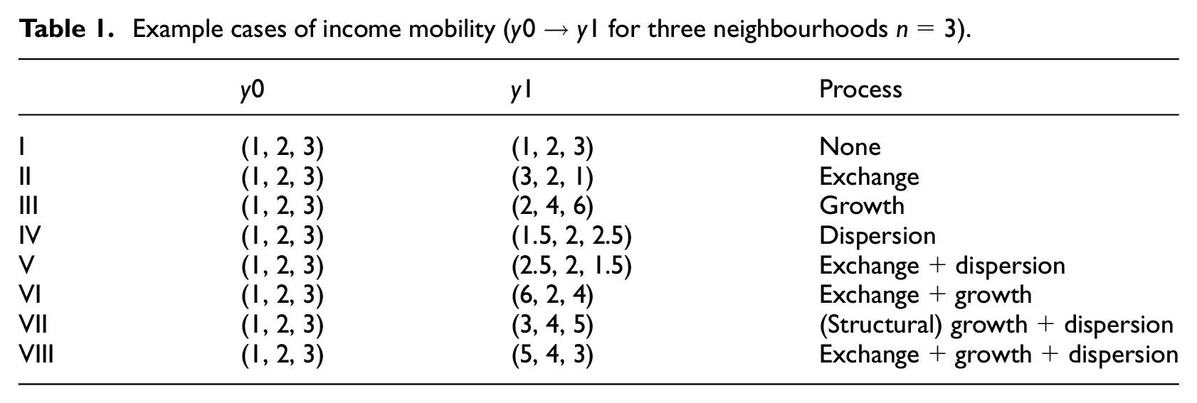
Analyses of structural mobility consider two properties of the income distribution: mean and dispersion. The former describes growth or decline in the city economy as a whole, while the latter relates to the changes in the shares each neighbourhood receives and is central to inequality dynamics. In Table 1 (
Fields (2006) identified six mobility concepts, which are time dependence, positional movement, share movement, income flux, directional income movement, and mobility as an equaliser of long-term incomes. Each captures one or more underlying processes (exchange/growth/dispersion). Despite lively inquiry into each of the six dimensions, different income indices are not comparable and the question of finding the dominant process or force driving overall income mobility remains unresolved. To address this gap, we leverage a decomposition technique to separate an income mobility measure into its underlying exchange and structural (and further, growth and dispersion) processes as components of the combined measure (Fortin et al., 2011). Using this framework, the components are comparable and we can evaluate which process dominates changes in the income distribution over a given time period.
Measure of income flux
We select an income flux measure to decompose and analyse if it is sensitive to all three processes. Income flux is concerned with the degree to which neighbourhood incomes remain stable over time. Since it does not differentiate gain from loss, it is also referred to as ‘non-directional income movement’. The measure of income flux we consider in this article is based on the absolute difference in log incomes (Fields and Ok, 1999). This measure has several useful properties – an important one is subgroup decomposition. Suppose we have
The difference in logs takes the initial incomes into account, as a dollar change would be relatively smaller for a higher initial income compared with a lower initial income.
A hierarchical decomposition
Our approach is to decompose the income flux measure
where
Exchange process
The counterfactual income vector

Structural process
The counterfactual income vector

Shapley procedure
Both equations (3) and (4) are first-round marginal effects and they do not necessarily add up to the income flux measure
Growth and dispersion processes
To further decompose the Structural component

and the second-round marginal impact of the Dispersion process is equal to
To obtain the first-round marginal impact of the Dispersion process, we construct the counterfactual income vector

and the second-round marginal impact of the Growth process is equal to
We apply the hierarchical Shapley procedure, which evaluates the primary factors
Jackknife resampling inference
We adopt the Jackknife resampling technique for estimating the standard errors of the income flux measure as well as the three contributory factors. We consider each pair of incomes in
Results: Neighbourhood income mobility
Among the
Descriptive statistics of real per capita incomes of urban census tracts in the US.

The estimate of the overall income mobility (income flux) in the long term (1980–2010) for
Neighbourhood income mobility decomposition in the long term (1980–2010).
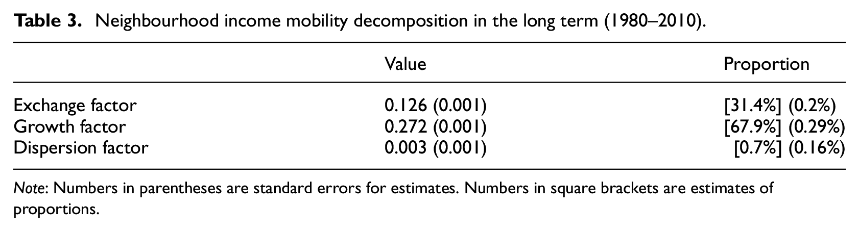
Note: Numbers in parentheses are standard errors for estimates. Numbers in square brackets are estimates of proportions.
These results are averages taken over all neighbourhoods from the 54,275 tracts. We now turn to a more granular examination of the spatial and temporal patterns of neighbourhood income mobility.
Global and local spatial analytics
After estimating the income flux measure and its three contributory components for each MSA, we proceed with exploratory spatial analytics to examine their spatial distributions. Here, we are interested in whether MSAs which have experienced more drastic changes in neighbourhood economic status are spatially proximate to those having a similar experience. This provides a sense of regional and local economic development modes, and could have important implications for the regional/local policy. We adopt the widely used Moran’s I, a global indicator of spatial association, to evaluate global spatial autocorrelation of the MSA income influx estimates as well as the proportions of the Exchange, Growth and Dispersion mobility components. For
where
Next, we decompose the global Moran’s I statistic into its local variety – Local Moran’s I (Anselin, 1995) – to further investigate whether hot or cold spots exist, with geographic clusters of MSAs with high or low neighbourhood income mobility. The local Moran’s I statistic for the variable
Inference is based on the pseudo-p value obtained from the conditional randomisation where for a focal MSA
The estimates of overall urban income mobility (income influx measure) for 291 MSAs display considerable variation, ranging from
The property of positive spatial autocorrelation also applies to the proportions contributed from the Exchange, Growth and Dispersion factors. The Growth factor has the widest range – [0.08, 0.91], indicating that the neighbourhood income mobility of some MSAs is dominated (as large as
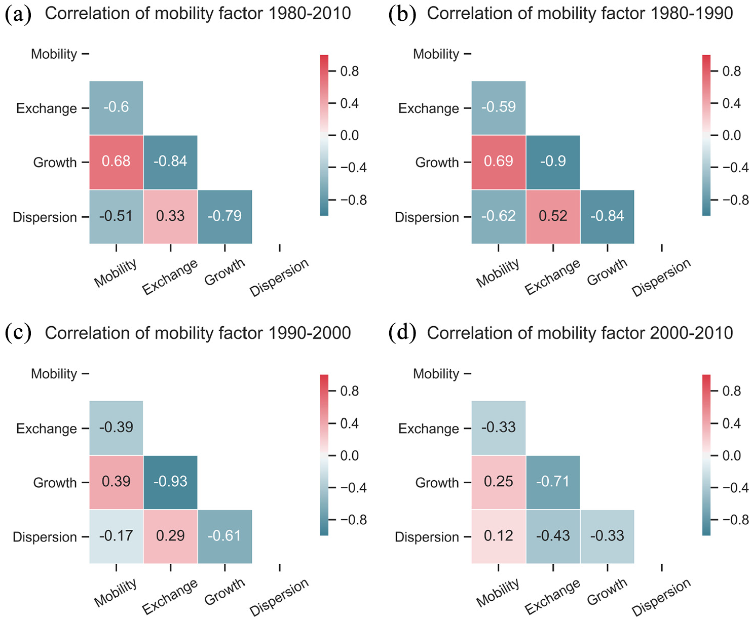
Correlation coefficients between mobility and its contributing factors. (a) 1980–2010. (b) 1980–1990. (c) 1990–2000. (d) 2000–2010.
Based on the local Moran’s I statistic while using spatial weights based on the eight nearest neighbours,
7
we identify hot and cold spots of MSAs in terms of the overall mobility level as well as the contributing proportions of the Exchange, Growth and Dispersion factors. Having controlled the false discovery rate (FDR) to deal with the multiple testing issue, we identify hot and cold spots for each term at the
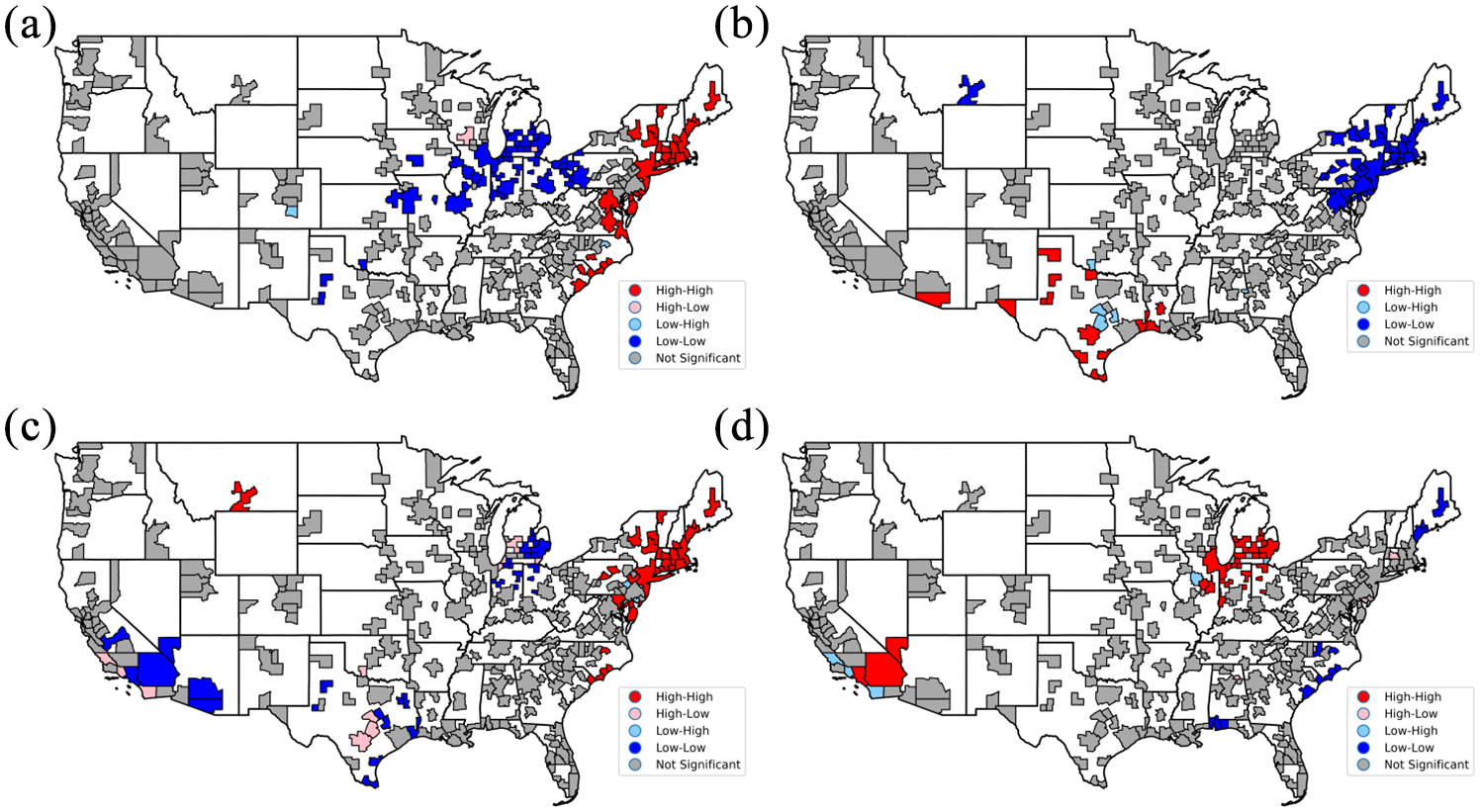
Local hot and cold spots of US MSA income mobility and the proportions of exchange, growth and dispersion mobility components across 1980–2010. (a) Income flux mobility levels. (b) Exchange mobility proportions. (c) Growth mobility proportions. (d) Dispersion mobility proportions.
Temporal heterogeneity
There are substantial differences in the decennial income movement patterns (across every two consecutive census years) as displayed by the black line in the left plot of Figure 3. In fact, the overall income mobility has been decreasing over time, indicating that urban neighbourhood income distributions have become more resistant to change. This decreasing trend also holds for the decennial growth rate (red curve). Contributions from the Exchange, Growth and Dispersion mobility processes have also been shifting over time. During the 1980–1990 period, the dominant process was Growth, as indicated by the yellow area in the right plot. Its dominant position was eventually replaced by the Exchange process (green area) during the 2000–2010 period. Over the three decades, the contribution from the Dispersion process (blue area) gradually increased, indicating that the income shares owned by urban neighbourhoods were transformed more drastically in recent decades.
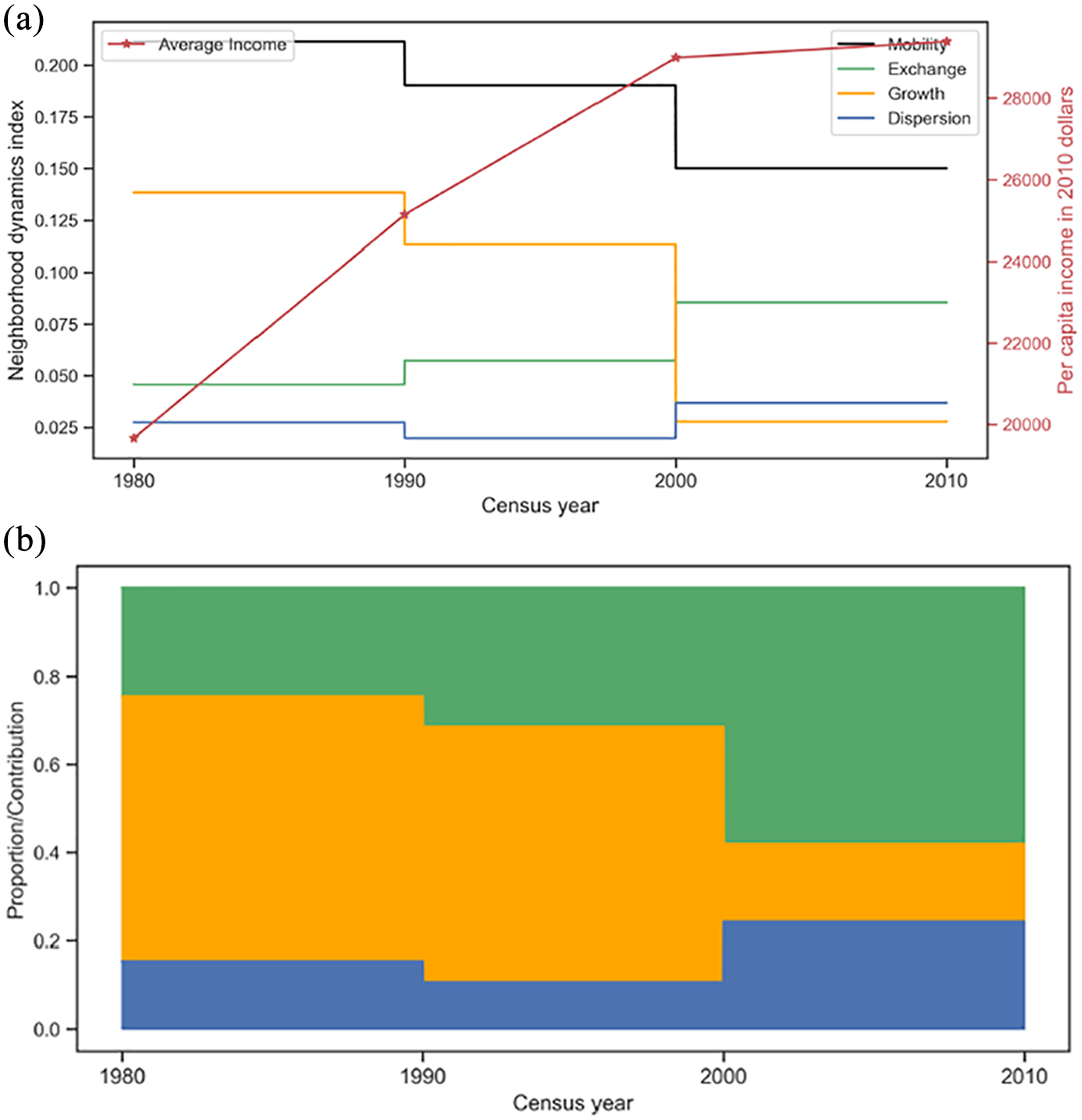
Average multidimensional neighbourhood dynamics across all MSAs under study. (a) Average multidimensional neighbourhood income dynamics across all MSAs. (b) Averages of contributions of exchange, growth and dispersion processes across all MSAs.
The pronounced temporal heterogeneity in the contributing proportions of three mobility components also manifests at the MSA level. Since the three proportions
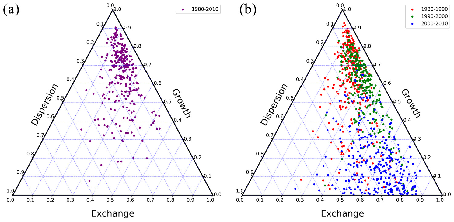
Ternary diagrams for proportions of exchange, growth and dispersion mobility components (a) in the long term 1980–2010, and (b) in the short terms 1980–1990, 1990–2000 and 2000–2010. (a) Long-term ternary diagram. (b) Decennial ternary diagram.
Spatial distribution of decennial MSA income mobility and the decomposition
Similar to the case with the long-term analysis, we also decompose national-scale urban income mobility into the MSA-scale, followed by a further decomposition into three contributing mobility processes. 8 The spatial patterns are most distinct for the first decade 1980–1990 in terms of the number of hot and cold spots detected. Similar to the long-term spatial pattern, the Northeast coast stood out as a hot spot for the overall mobility level and Growth mobility, and a cold spot for Exchange and Dispersion mobility. By contrast, the Great Lakes region failed to stand out; instead Texas, New Mexico and Louisiana hosted cold spots of Growth and hot spots of Exchange and Dispersion. In the next decade (1990–2000), we observe cold spots for overall mobility and Growth mobility, as well as hot spots for Exchange mobility in the West coast. For the most recent decade 2000–2010, the Great Lakes region stood out as the host of MSAs with high contributions from Growth mobility and low contributions from Exchange mobility.
The relationships between the overall mobility level for each MSA, and the proportions contributed from Exchange, Growth and Dispersion mobility processes across each decade have also undergone drastic changes as shown in Figure 1. Though the relationship between the income flux level and the Growth contribution has been always positive, it has weakened over time. Another noticeable change comes from the relationship between the Dispersion and the other two components. Over the three decades we study, the initial negative relationship between Dispersion and Growth has been gradually replaced by a weak positive relationship, while on the contrary, the initial positive relation between Dispersion and Exchange has been replaced by a negative relationship.
Generalising neighbourhood income mobility
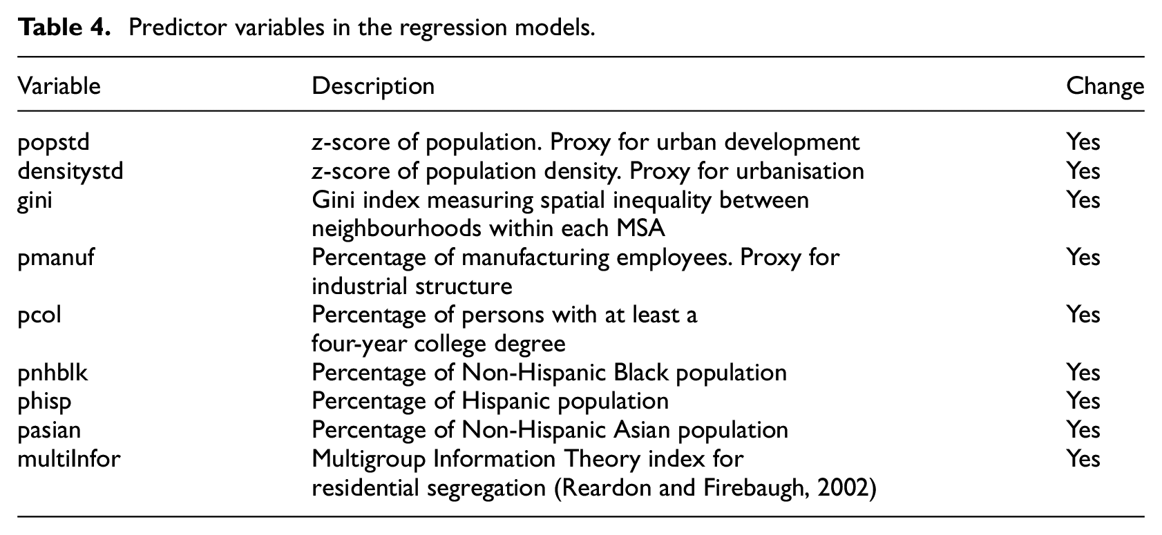
Given the widespread temporal and spatial heterogeneity in the neighbourhood mobility results that we have identified, we carry out a spatial econometric analysis as a first step to identify the possible factors that may be driving neighbourhood income dynamics in urban US regions. Compared with spatial income inequality (Rodríguez-Pose and Ezcurra, 2010; Wei, 2015), scholarship on income mobility at the spatial aggregate level is considerably limited. We address this gap by formally modelling the relationship between the metro-level income mobility (and its contributory components) and the metro-level variables at the beginning year of each decade listed in Table 4. These nine variables cover urban development, spatial income disparity, industrial composition, education attainment and residential racial composition and segregation. We have also tested against the decadal changes in these variables, leading to another set of models with 18 predictor variables. 9
Predictor variables in the regression models.
Our point of departure is the classic linear model in equation (10) specified for each mobility measure (


The estimation results for these specifications for the three decades are reported in Tables 5 to 7. The results mirror the temporal heterogeneity seen in our exploratory results in that factors that are associated with neighbourhood income mobility vary over the decades. For example, the percentage of manufacturing employment has only been significant for the period 1980–1990 as shown in Table 5. After incorporating its decadal increase in the model (model II), manufacturing employment was positively related to the spatial income influx level and Growth mobility. Racial composition including the percentages of Hispanic and Asian, the racial segregation level, and higher education attainment were only significant in the latest time period 2000–2010 (Table 7). While the initial percentage of Hispanic population was negatively related to the spatial income influx level and Growth mobility, the story was the opposite for the initial percentage of Asian population. Residential segregation was (weakly) negatively related to the spatial income influx level and Dispersion mobility, potential evidence for a stagnating effect of segregation on neighbourhood income mobility.
Correlates of urban income mobility 1980–1990 (spatial lag specification with maximum likelihood estimation).
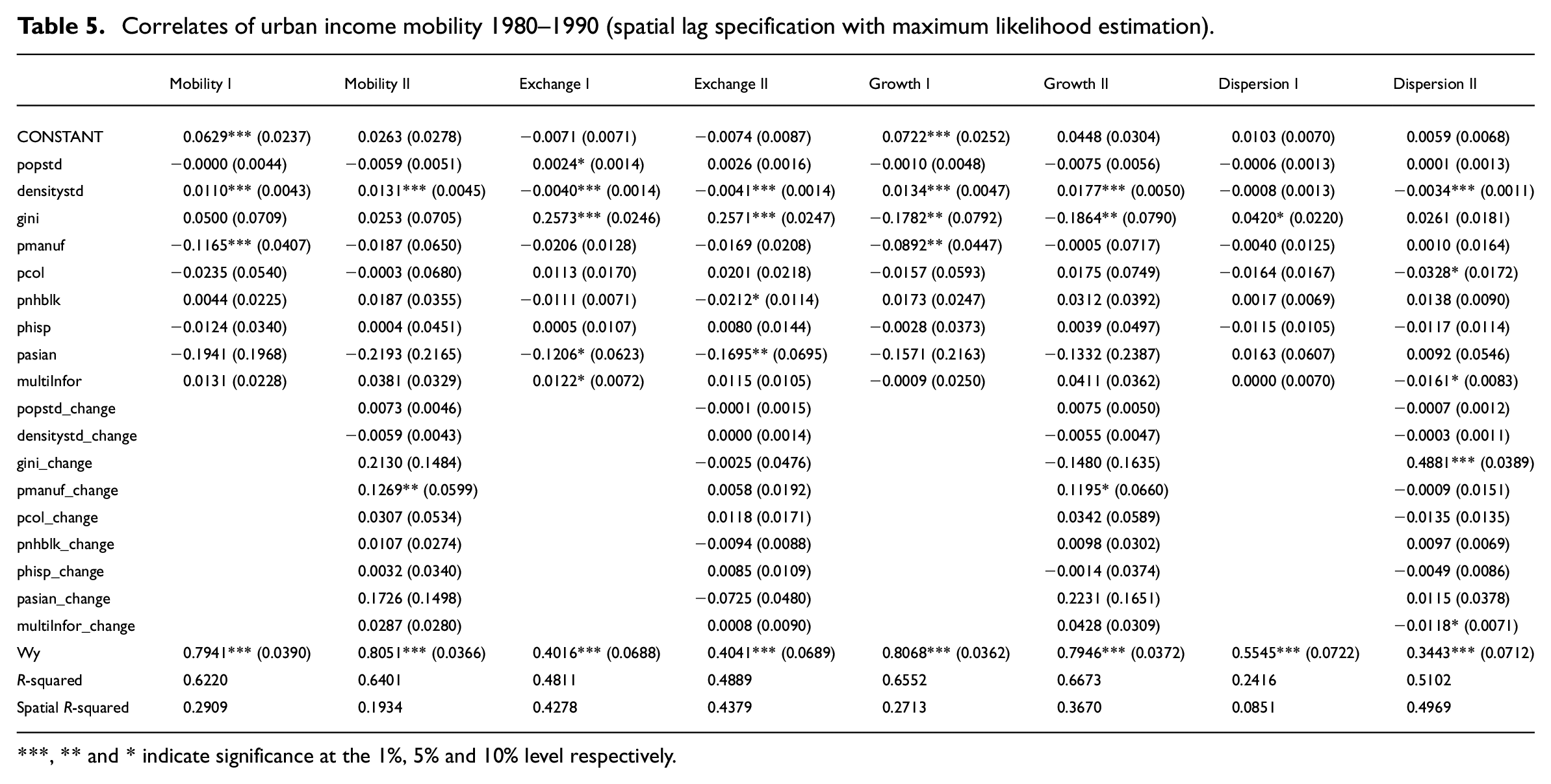
** and * indicate significance at the
Urban development level proxied by population and population density was significant for 1980–1990 and 2000–2010. It was positively correlated with the overall neighbourhood income dynamics and Growth mobility, and negatively correlated with Exchange and Dispersion mobility for 1980–1990. While for 2000–2010, the increment in population density was negatively correlated with the overall neighbourhood income dynamics, the initial population was positively correlated with Exchange mobility.
Comparatively, the level of spatial income inequality was the only factor significant across all three decades. Initially across 1980–1990, it was positively correlated with Exchange mobility and negatively correlated with Growth mobility, while its decadal increment was positively correlated with Dispersion mobility. The pattern was similar in the subsequent periods 1990–2000 (Table 6) and 2000–2010 (Table 7). One prominent observation is that in the last decade (i.e. 2000–2010), the level of spatial income inequality and its decadal increase was also positively correlated with the overall neighbourhood income dynamics.
Correlates of urban income mobility 1990–2000 (spatial lag specification with maximum likelihood estimation).
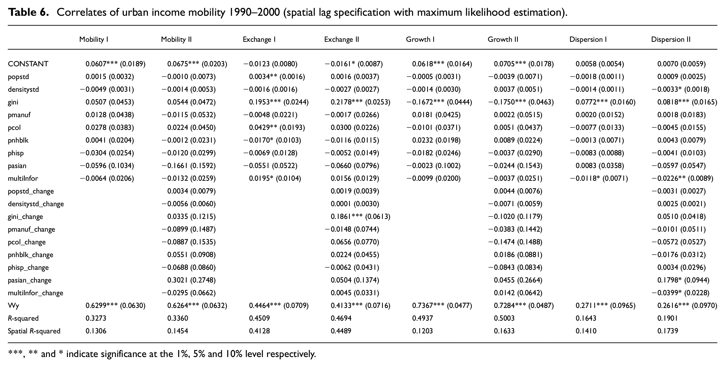
** and * indicate significance at the
Correlates of urban income mobility 2000–2010 (spatial lag specification with maximum likelihood estimation).
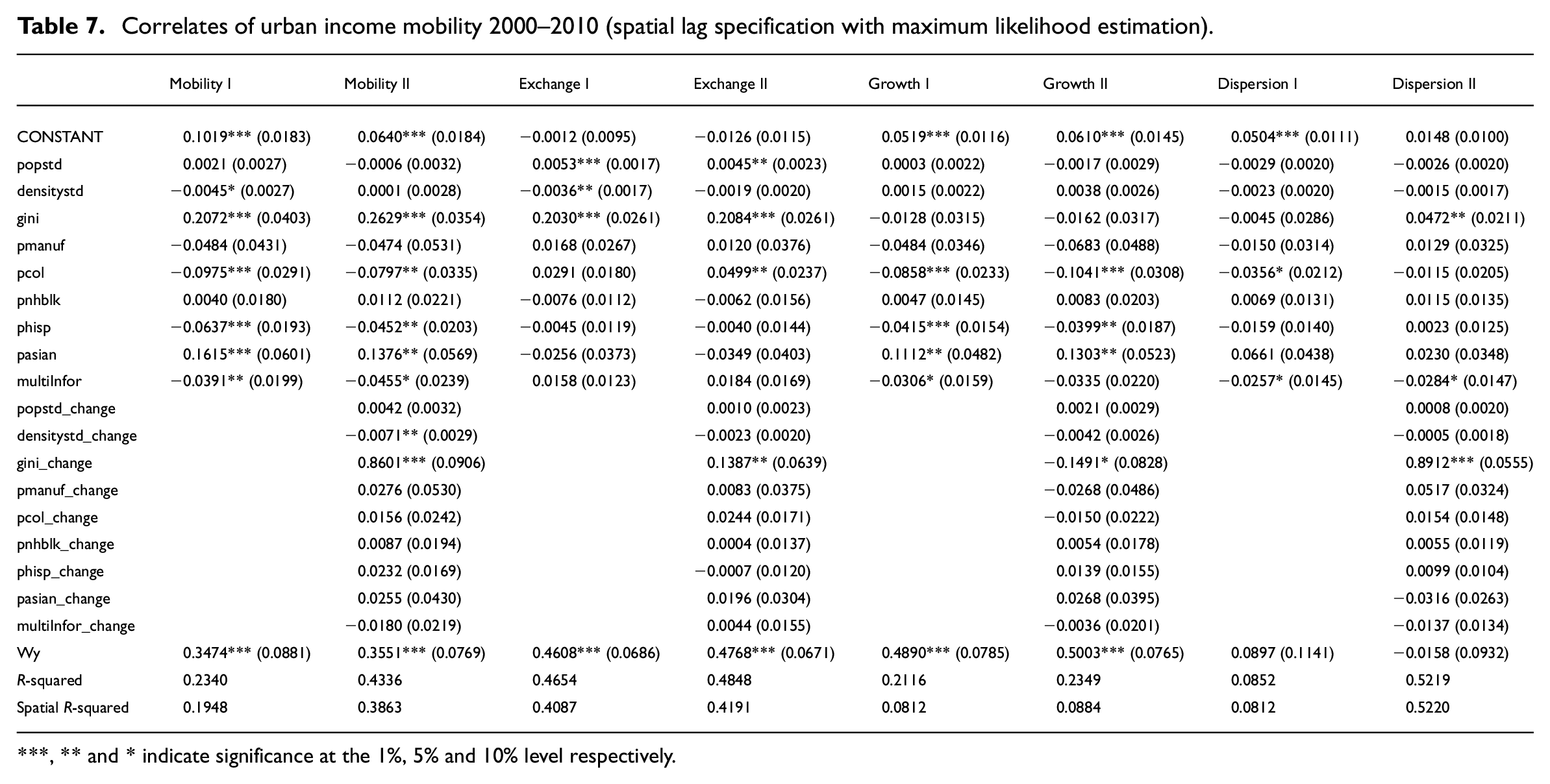
** and * indicate significance at the
There is strong evidence of spatial dependence across all three decades. The spatial lag is significant for all types of MSA-level neighbourhood mobility measures, with the only exception being the dispersion component in the final decade. This form of dependence reflects the regional patterning we found earlier in the hot (cold)-spot analysis. The temporal constancy of the spatial dependence stands in stark contrast to the temporal heterogeneity reflected in the other correlates of neighbourhood income mobility.
Discussion
Our results provide intriguing insight into the dynamics of spatial inequality in American cities over the last three decades that have not been explored in the literature, particularly when examining different spatial and temporal scales. Our results highlight the considerable ways that the American urban economy has differed over space and changed through time, and elucidate the ways in which different regions of the country have borne witness to unique changes as they move through certain time periods.
We can view these results in a broader historical context. Through the early part of the 20th century, America’s economy rose to prominence thanks to a dominant manufacturing sector that flourished throughout the Midwest, particularly in prominent cities like Chicago, Detroit, Cleveland, Pittsburgh and Milwaukee. The primary demographic trend during this period was ‘white flight’, or the suburbanisation of white, well-educated and affluent families (Baum-Snow and Hartley, 2020). Through the new millennium, however, as the country shifted away from manufacturing and embraced a high-tech digital and information economy, Midwestern dominance waned and eventually the Midwest developed the ‘rustbelt’ moniker for its legacy and aesthetic of factories, foundries and warehouses beginning to fall into disrepair.
In our current era, this demographic trend has thus largely reversed, thanks to the ‘back to the city’ movement and the dominance of new high-tech job hubs like San Francisco and Seattle that have overtaken Midwestern cities in cultural and economic dominance (Ehrenhalt, 2012). These trends are a particularly useful context for interpreting our results on the spatial and temporal patterns of economic mobility because they highlight (1) the important regional nature of American economics and demography, (2) the important temporal phases that define the country’s economic history, and (3) the relationship between space and time in laying the foundation for the economic mobility of American neighbourhoods.
Over the long term (1980–2010) our results are consistent with these economic and demographic narratives. The Northeastern megaregion showed little evidence of internal restructuring in that it hosted cold spots for exchange mobility. At the same time, however, it hosted hotspots for growth mobility. At a local scale, this means that neighbourhoods in New York and Washington DC did not trade ranks often; prominent neighbourhoods in New York and DC stayed as such. On a national scale, however, these same cities continue to outpace smaller, and more centrally located ones, like Detroit, that were once dominant on the national scale. Indeed, the Midwest displayed largely the opposite patterns, representing a statistical cold spot for overall mobility over the full 1980–2010 time period and, similarly, a cold spot for growth.
Economists and geographers have long recognised the importance of agglomeration economies in helping to foster economic growth, but our results are the first of which we are aware that demonstrate the statistical significance of these meso-scale economic regions whose metropolitan statistical areas tended to follow similar mobility trends. Indeed, these results have strong implications for (mega)regional economic development policy and national economic inequality more broadly, but we also find considerable nuance within each decade, which we explore below.
In the 1980s, deregulation and the transitioning economy led to reshaping of urban inequality across the US, metropolitan regions with larger shares in manufacturing employment saw an overall decrease in economic mobility, whereas economic deregulation led to considerable growth in financial centres along the Northeast corridor. Metropolitan regions with larger populations and denser development were positively associated with growth and negatively associated with exchange and dispersion. Put differently, large, dense cities on average, did quite well in the 1980s, with most neighbourhoods moving up the economic ladder together, albeit with few changes in position. The Northeast megaregion stood out as a statistically significant hotspot in this respect, as nearly all of the major metropolitan regions along the seaboard experienced these trends together. For smaller and more rural parts of the country, however, a different story emerges. In metros with large shares of the economy dedicated to manufacturing, neighbourhoods generally saw an economic decline. Portions of the South and Midwest stood out as spatially significant hotspots for dispersion and widening inequality, whereas the rustbelt in Western Pennsylvania stood out as a significant cold spot for economic growth.
The 1990s seemed to be a period of polarisation and widening inequality, with the gap growing fastest in places already characterised by a high spatial Gini index. Further, metropolitan regions with large college-educated populations saw a larger change in economic dispersion. Many of the largest metros in the 90s seemed to be characterised by widening inequality, as low-tech, high-paying jobs in the manufacturing sector began disappearing from high-cost cities. Together, those trends were consistent with a narrative describing the reshuffling of affordable neighbourhoods on the national scale along with the nascent origins of the ‘back to the city’ movement, two trends that together had sweeping implications for gentrification and urban displacement in the following decade (Hyra, 2015; Sturtevant and Jung, 2011).
Indeed, through the new millennium spatial trends in economic mobility continued apace, albeit with a newly emerging racial patterning in which areas with large Hispanic and Latino populations were insulated from economic growth whereas areas with large Asian populations accelerated. As with the 1990s, cities in the 2000s that had large shares of college-educated citizens were more likely to experience dispersion and a lack of economic growth. This also applied to growing inequality, as cities that already had large spatial Gini indices were more likely to continue a trend towards exchange and dispersal. In other words, through the 2000s, many of America’s most unequal cities grew even more so. From a spatial perspective, there was considerably less statistical patterning, although a significant pattern of exchange mobility emerged through Silicon Valley and the Detroit metro region.
Although our results show nuance in each decade, some long-term trends are nonetheless important to discuss. In particular, while the spatial and economic consequences of deindustrialisation have been explored at length in the urban economic literature (Dawkins, 2003), a critically underexamined component of economic restructuring has been its impact on prevailing political ideology and the spatial patterning thereof: a phenomenon Rodríguez-Pose (2018: 189) has called ‘a wave of political populism with strong territorial, rather than social foundations’. The result, as Rodríguez-Pose describes, is that political persuasions have polarised in the US and elsewhere, revealing a pattern in which ‘populism took hold not among the poorest of the poor, but in a combination of poor regions and areas that had suffered long periods of decline. It has been thus the places that don’t matter, not the “people that don’t matter”, that have reacted’ (2018: 201). Our findings underscore this perspective. While the American rustbelt was once an engine of economic opportunity, providing high paying jobs in manufacturing and mining, our results demonstrate a sustained period of slow growth, whose explicitly regional manifestation carries political implications for the electoral map, as well as for national unity and inequality.
Conclusions
This paper provides an empirical study of US neighbourhood income dynamics using decennial census and American Community Survey (ACS) datasets covering a variety of mega, medium and small cities over both long-term time spans (1980–2010), as well as short terms 1980–1990, 1990–2000, 2000–2010. We adopt a decomposition technique for unpacking an overall spatial income mobility index into its contributing components (namely Exchange, Growth and Dispersion mobility) to obtain insights into processes of multidimensional urban and neighbourhood change. The paper represents one of the first comprehensive studies of neighbourhood income dynamics in the metropolitan United States, covering a broad set of cities and a variety of temporal scales and using spatially explicit exploratory and confirmatory analytics.
We find that, at the national scale, Growth mobility dominates followed by Exchange mobility in the long term. However, this dominating–dominated relationship is reversed over time in the short term, indicating temporally heterogeneous urban and neighbourhood processes. We confirm this temporal heterogeneity by examining MSA-level spatial mobility. In the long term, we uncover a strong negative relationship between Growth and Exchange/Dispersion mobility, while Growth mobility appears positively related to overall spatial mobility. Together these findings indicate that more mobile MSAs were typically dominated by changes in absolute average income level, and these MSAs tend to host tracts with fewer rank exchanges or changes in income shares. These relationships, however, have been changing in shorter time frames, a finding we confirm through a set of regression analyses demonstrating temporal variation in statistically significant determinants. This finding, we argue, stresses the importance of studying urban processes through a dynamic lens. Aside from temporal heterogeneity, another significant finding is the spatial agglomeration effect of intraurban neighbourhood income dynamics; for example, the Northeastern and the Great Lakes regions have been hosting either hot spots or cold spots of neighbourhood income dynamics and its contributing components.
As we demonstrate in the paper, different temporal scales can manifest diverging neighbourhood income patterns and thus varying urban and neighbourhood dynamics. While we look at a 30-year long term, as well as the three decadal short terms, we lack information on smaller temporal scales, such as the five-year mobility, or even the yearly mobility, which could be the defining force or turning point in the more extended period. An interesting endeavour would be to utilise the ACS five-year estimates (2009–2018) to investigate smaller temporal scales though this comes with the downside of dealing with larger margins of error. Another limitation of the current paper is the limited set of explanatory variables adopted for the spatial regression analysis. A promising avenue for further research is, thus, to interrogate household migration across neighbourhoods and MSAs, which may provide a better sense of how the observed neighbourhood income dynamics, as well as the Growth, Dispersion, Exchange components, relate to demographic processes such as gentrification or displacement. Another interesting dimension is to explore whether and how institutions as well as technology and innovation have been shaping smaller-scale inequality dynamics, as they have been demonstrated to impact dynamics at the larger scales (Lee and Rodríguez-Pose, 2016; Rodríguez-Pose, 2013; Storper et al., 2015).
Future work should also consider a spatially explicit view of neighbourhood inequality dynamics within MSAs. Although the decomposition method we present here allows for a comprehensive analysis of multiple neighbourhood processes within each MSA, it falls short of shedding light on potential spatial spillovers. In other words, it does not provide insights into whether nearby neighbourhoods tend to move together in ranks, absolute income growth, or income shares. Future research could be directed to a further decomposition of the current measure, which will enable a spatially explicit view or an application of extant spatially explicit income mobility measures (Kang and Rey, 2020; Rey, 2016).
Footnotes
Declaration of conflicting interests
The author(s) declared no potential conflicts of interest with respect to the research, authorship, and/or publication of this article.
Funding
The author(s) disclosed receipt of the following financial support for the research, authorship, and/or publication of this article: This material is based upon work supported by the National Science Foundation under Grant BCS 1759746.