Using Quantile Regression to Understand Visitor Spending

Abstract

A common approach to assessing visitor expenditures is to use least squares regression analysis to determine statistically significant variables on which key market segments are identified for marketing purposes. This was earlier done by Wang for survey data based on expenditures by Mainland Chinese visitors to Hong Kong. In this research note, this same data set was used to demonstrate the benefits of using quantile regression analysis to better identify tourist spending patterns and market segments. The quantile regression method measures tourist spending in different categories against a fixed range of dependent variables, which distinguishes between lower, medium, and higher spenders. The results show that quantile regression is less susceptible to influence by outlier values and is better able to target finer tourist spending market segments.

Keywords

quantile regression least squares regression Hong Kong tourist expenditures Chinese tourists market segmentation

Tourism is a basic export industry. It is a basic industry because almost all of the income generated by tourism comes from local products and experiences sold to customers who pay for them with money earned outside of the local community (Hall and Lew 2009). Traditional basic industries include primary activities, such as agriculture and mining, as well as manufacturing and sales to the degree that they are exported and sold to people and entities who earn their livelihood outside of the community. Tourism is a form of export industry, even though its products are consumed in situ (at the site of production) and are not physically exported. What is important is that a purchase is made of local products (or experiences) by consumers who normally reside outside of the community. Basic export industries are important to the economic well-being of a community, because without an external source of income, leakages may gradually drain the local economy of resources.

The argument that tourism activities effectively increase the gross wealth or income of a community is what makes tourism a popular form of economic development (Frechtling 1994). Economic leakages, such as when tourists purchase products that are imported into the local economy, can significantly decrease the potential benefit of tourist expenditures. In fact, much of what a tourist purchases has a high import content, from transportation and fuel on the trip from their home, to accommodation facilities made from imported steel and wood, to restaurant foods and souvenirs grown and made in distant lands.

Despite the complexities in understanding the full economic impacts of tourism, the essence of the tourism economy is clearly built on the expenditures made directly by tourists in the destination. Segmenting the tourist market on the basis of expenditure patterns is, therefore, an important and common approach to understanding the economic impacts of tourism on a destination (Weber 1995) as well as expanding its economic benefits. Such segmentation is often undertaken with the goals of assessing visitor destination or shopping satisfaction (Heung and Cheng 2000; Wong and Law 2003; Joppe, Martin, and Waalen 2001), identifying “big spenders” (Legohérel and Wong 2006; Díaz-Pérez, Bethencourt-Cejas, and Álvarez-González 2005; Wicks and Schuett 1993), or trying to determine if one part of a tourist population spends more or differently than another part (Agarwal and Yochum 1999). For many such studies, market segmentations are based solely on the visitor country of origin, and the numeric variations in expenditures are simply the overall mean values or purchase category mean values for the respondent groups (Suh and Gartner 2004).

For example, Rosenbaum and Spears (2005) used analysis of variance (ANOVA) to examine variations in expenditure patterns among different nationalities visiting Hawaii and found that Japanese visitors on average were not only the biggest spenders, by far, but also planned to stay longer in Hawaii and spend more time shopping there than any other group during the survey period. They also found that repeat visitors on average planned to spend more in Hawaii than first-time visitors. Other common independent variables used to segment market populations include income, age, and gender (Lehto et al. 2004; Mok and Iverson 2000); tourist interests (Mehmetoglu 2007); and trip type (Oh et al. 2004). A separate set of studies consists of those that model changes in overall tourist expenditures at a destination over time (Narayan 2005; English 2000).

Our present study takes one element in a market segmentation survey, tourist expenditures, and provides a different analysis of that variable. In that sense, this is not a market segmentation study but is instead an application of a statistical methodology to provide a more robust understanding of the determinants of tourist spending. We believe that this alternative approach can provide additional insight into the key variables in tourist expenditures, especially in a setting such as Hong Kong where mainland Chinese tourists are both large in numbers and diverse in their income levels (Wang 2004; Yoo, McKercher, and Mena 2004). Mainland Chinese visitors comprise more than half of annual hotel nights in Hong Kong and are the territory’s highest spending visitors (Chan 2008). For most mainland visitors, Hong Kong is a shopping destination and a frequent last stop before returning home from an overseas trip (Lew and McKercher 2002). When one tourist origin source is so important to a destination, then a finer analysis of their expenditure patterns is warranted.

In most tourist expenditure studies, the statistical significance of differences between market segments has been based on least squares regression. However, least squares regression is designed to estimate only the average (mean) spending behavior across groups of tourists. Since not all tourists behave like an average tourist, it is valuable to find out not only the average difference across groups but also the differences between the higher and lower ranges within the groups. For our analysis of tourist expenditures, this is the difference between the big spenders and the more frugal spenders, after controlling for variations in demographic characteristics. Knowing the behavior of big spenders in comparison to frugal spenders can potentially help tourism planners achieve higher impacts in their advertising and travel programs.

Recently, Perlich et al. (2007) illustrated how high-quantile modeling can be practically important in “customer wallet estimation” (i.e., estimation of potential spending by customers) as compared to estimating the expected (mean) spending using traditional least squares regression and described a wallet estimation implementation within IBM’s Market Alignment Program. They argued that “when modeling sales prices of houses, cars or any other product, the seller may be very interested in the price they may aspire to get for their asset if they are successful in negotiations. This is clearly different from the ‘average’ price for this asset and is more in line with a high quantile of the price distribution of equivalent assets. Similarly, the buyer may be interested in the symmetric problem of modeling a low quantile.” Applied to our setting, policy makers and entrepreneurs in the travel industry may be more interested in knowing how much potential revenue they can aspire to extract from tourists via high-quantile modeling rather than how much revenue they can expect to deduce from visitors via traditional least squares regression estimates.

The standard deviation and range are other measures of dispersion that can provide a rough indication of the degree of spread among extreme values around the mean. In addition, a least squares regression can control for the effect of additional independent variables on the average spending category. However, a richer and more precise understanding can be achieved through quantile regression analysis, which allows examining and comparing different levels of response given the variation in the independent variables. Respondents who only spent, for example, 10% of the mean on meals outside of their hotel can be directly compared with those who spent twice the mean, and those who spent exactly the mean amount, holding all the other factors fixed.

Using quantile regression, we were able to see the different spending behavior across the whole spectrum of the tourist population, from the big spenders, through the moderate spenders, and to the frugal spenders, among Mainland Chinese visitors to Hong Kong. For example, we found that the number of previous visits had significant increasingly positive effects on the middle 50% of the shopping spending distribution, and being a repeat visitor increased shopping spending more for heavier spenders than for the more frugal. Duration of stay, however, was found to not have a significant effect on shopping spending behavior overall. It was also found to not have a significant impact on spending for meals outside hotel and hotel bills for an average spender, although it did have significantly increasing positive effects on the upper 60% of the distribution in spending for meals outside of hotels and spending for local transportation, and increasing positive influences on the top 30% of the hotel spending distribution. Thus, efforts to increase the stay of Mainland Chinese visitors would mostly affect the amount of money they spend on food outside of their hotel and on transportation, at least among the middle and higher spenders. Also the hotels that cater to big spenders would also benefit more than average from longer stays by their Mainland Chinese clientele.

We furthermore found that the age 26 to 40 group of visitors had higher spending on shopping than the other age groups across the whole distribution, and the top 10% of the spenders (i.e., the big spenders) among them spent ten times as much as the bottom 10% (frugal spenders), when compared to the other age groups. This suggests that focusing the shopping promotional campaign on this particular group of Mainland Chinese visitors could have a greater impact on Hong Kong tourist expenditures.

The rest of the paper is organized into the data and methodology section, followed by the section on the major findings for shopping and overall expenditures. Other spending categories, as discussed briefly above, were also examined, but are excluded here for brevity. The details of those additional findings can be found online in Ng and Lew (2009). The last section discusses implications of the quantile regression approach and results for policy makers and other tourism entities.

Data and Method

At the household or family level, economic theory typically depicts consumption level as being determined by socioeconomic factors, such as income, wealth, age, education, family size, expectation about the level and risk of future income or wealth, and personal interest. In this study, therefore, the consumption level ( y_i) of the ith individual, measured in turn by spending on shopping, meals outside hotel, local transportation, and on hotels, is formulated as a function of k socioeconomic factors in the k vector x_i as follows:

y_{i} = f (x_{i}),

where x_i includes occupation, length of stay, and number of visits. These are treated as a rough proxy for income, age, and education levels, with higher status occupations, longer stays, and more frequent visits collectively approximating higher income, age, and education (Wolff 2006).

The data used in this study were the same as those used in Wang (2004), which were extracted from the visitors’ survey conducted by the Hong Kong Tourist Board (HKTB) in 1999. The 634 Mainland Chinese vacationers aged 16 or older who were interviewed face-to-face were randomly selected at four border control points: the Hong Kong International Airport, the Hung Hom Railway Station, the China Hong Kong Ferry Terminal, and the Macao Ferry Terminal. The number of respondents interviewed at each of the four control points was proportionate to the actual number of visitors who passed through the control points. The survey was implemented on a continuous basis, with a relatively equal number of interviews conducted in each month of the year.

Data on marital status were classified into married, never married, and other, which was used as the base so that the estimated regression coefficient for marital status could be interpreted relative to this category. The length of stay variable measured the number of nights the visitors stayed in Hong Kong during their current trip. Repeat visitors were identified by those whose number of visits to Hong Kong was at least two. Education level was classified into three levels: primary or no education, secondary/high school, and the base level college or above. Occupations were characterized by four dummy variables: professional/managerial, proprietor/owner, junior white collar, and blue collar, with the base level capturing other job types. Age group was broken down into age 16 to 25, age 26 to 40, age 41 to 60, and greater than 60, which was used as the base. Gender was split into female (as the base) and male.

To study tourist behavior on four major spending components (shopping, meals outside of hotels, local transportation, and hotel, all measured in U.S. dollars), Wang (2004) performed separate least squares regressions of the four components on the common set of independent variables that captured visitors’ socioeconomic characteristics (marital status, age, gender, occupation, and educational attainment), the length of stay, and the number of previous visits. His least squares regression results were presented in Table 7 of Wang (2004). Investigation of the variance inflationary factor (VIF) of the independent variables, however, revealed that the never-married dummy variable had the highest VIF value of 17.29, which suggests high correlation between this dummy variable and other independent variable(s). After dropping this dummy variable, we found that the dummy for age 26 to 40 had the highest VIF value of 12.28 among the remaining VIF values, followed by the VIF value of 10.46 for the age 41 to 60 dummy. We decided to drop the dummy for age 41 to 60 so that the base level for the age dummies became age 41 and older. After this, none of the remaining independent variables had a VIF value higher than 2.0, and there was no more evidence of multicollinearity among the remaining independent variables.

We performed a special case of the White test for heteroscedasticity by regressing the squared residuals on the fitted dependent variable and its squared term. The chi-square statistic when using the total spending, spending on shopping, spending on meals outside of hotels, spending on local transportation, and spending on hotel in turn as the dependent variable is, respectively, 19.20, 19.39, 33.34, 58.40, and 6.81. They all have essentially zero p values. Thus, there is extremely strong evidence of heteroscedasticity (a predictable change in variance over the distribution of the dependent variable) in the least squares regression models. To make sure that the heteroscedasticity test does not pick up the effect of functional form misspecification in the regression model, we performed the test by including the quadratic terms of length of stay and number of visits and logarithmic transformation on the dependent variable. The conclusions remained the same. Hence, we computed the Eicker-Huber-White heteroscedasticity-robust standard errors in all the least squares regression results below, which should be more reliable than those reported in Wang’s (2004) Table 7.

Because of the presence of heteroscedasticity, quantile regression becomes even more relevant as a tool to reveal any potential variation in the effect of the independent variables on the dependent variables over the various segments of the population. If there is no variation in the dispersion of the dependent variable across the different ranges of the covariates, the conditional mean is capable of revealing information on other quantiles of the conditional distribution with the addition of some parametric assumptions on the error term. In the presence of heteroscedasticity of any form, however, no parametric distribution model can reasonably be expected to capture the unknown conditional distribution to be useful for the estimation of the covariate effects in the other quantiles using the least squares regression. Quantile regression, on the other hand, is designed to capture any potential covariate effects in any chosen quantile and does not rely on any parametric specification of the conditional distribution.

Given n observations of the dependent variable y_i, and k independent variables represented by the k vector x_i for i = 1, . . ., n, the k vector of τth quantile regression coefficients, β(τ), minimizes

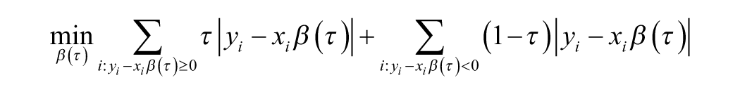
\min_{β (τ)} \sum_{i : y_{i} - x_{i} β (τ) \geq 0} τ | y_{i} - x_{i} β (τ) | + \sum_{i : y_{i} - x_{i} β (τ) < 0} (1 - τ | y_{i} - x_{i} β (τ) |

where 0< τ< 1 determines the desired conditional quantile of interest. In the objective function above, all positive residuals receive a weight of τ while the negative ones receive a weight of (τ−1). Hence, 100τ% of the dependent observations will fall above the τth quantile regression hyperplane and 100(1−τ)%below. For τ = 0.5, the quantile regression hyperplane bisects the dependent variable into two halves along the directions of the covariates such that half of the observations fall above while the other half below the regression hyperplane and yield the median regression estimates as a special case. Hence, any one of the k components of the quantile regression coefficients, β_j(τ), provides an estimate of the marginal effect of the associated independent variable x_j on the dependent variable for the τth quantile of the cohort holding the effects of the remaining independent variables fixed.

One common misconception on the computation of quantile regression coefficients is the impression that only τ% of the data points are used in the estimation of β_j(τ)and, hence, the different quantile regression coefficients are estimated with different sample sizes. However, this cannot be farthest from the truth. Just like every single data point is used in determining the median or any specific quantile for a single random variable, all the data points are used in the computation of the quantile regression coefficients. Quantile regression coefficients are typically computed by expressing the objective function stated above as a linear program, and then a simplex method (Koenker and d’Orey 1987; Ng 1996) or interior-point algorithm (Portnoy and Koenker 1997; Koenker and Ng 2005) can be applied. Other available approaches to compute the quantile regression coefficients are the majorize-minimize algorithm of Hunter and Lange (2000), the reversible jump Markov chain–Monte Carlo algorithm of Yu (2002), and the smoothing algorithm of Chen (2007), all using the whole data set.

Quantile regression software is readily available in most modern statistical platforms, including EasyReg, EViews, LIMDEP, SAS, SHAZAM, SPSS (via the SPSSINC QUANTREG extension package), STATA, and the GNU Free Software R for statistical computing and graphics (R Development Core Team 2008). All of the above except EasyReg and R are commercially licensed. EasyReg and R are free for noncommercial use. EasyReg, EViews, and STATA have point-and-click menu-driven interfaces while LIMDEP has a menu for command builder only, SHAZAM can be made menu driven via SHAZAM Wizards and SAS/ASSIST provides SAS users with a menu-driven interface. The majority of the platforms are not user expandable, with the exceptions that users can expand SAS’s capability via integration to R, STATA is user expandable via its ado-files, and R is a fully user-expandable programming environment. All quantile regression coefficients in this study were computed using the QUANTREG package (Koenker 2009) available for R because it is the most flexible computing platform for frontier research and has a very large collection of user-contributed packages (more than 2,500 at this writing). The algorithm uses a modified version of Barrodale and Roberts’s (1974) simplex algorithm for L₁ regression as described in Koenker and d’Orey (1987, 1994) and the interior-point algorithm as depicted in Koenker and Ng (2005). The standard error presumes local linearity of the conditional quantile functions and computes an Eicker-Huber-White sandwich estimate using a local estimate of the sparsity. See Koenker and Hallock (2001) and Yu, Lu, and Stander (2003) for a cogent, nontechnical introduction to quantile regression.

Results

The least squares regression (LSR) and quantile regression (QR) estimated coefficients are presented in Tables 1 and 2 for the dependent variable spending for shopping and total spending, respectively. Since there is a plethora of numbers in the tables, we present the information graphically in a more parsimonious way in Figures 1 and 2. The tables show the nine distinct deciles representing 10% increments in τ along the distribution. Each panel in a figure presents the quantile regression estimates for the coefficients of a covariate. For each of the covariates, 17 distinct quantile regression estimates for τ ranging from 0.1 to 0.9 in increments of 0.05 are plotted as solid dots joined by a solid line. We do not include estimates of the extreme 0.05 and 0.95 quantile coefficients in this study because of the low precision in the estimates of the coefficients near the boundaries of the extreme quantiles caused by the fact that conventional large sample theory for quantile regression does not apply far into the tails of the distribution (Chernozhukov 2005). As a result, our results do not extend without caveat to extremely high or extremely low spenders in the four categories of spending that we have studied.

Figure 1.

Least squares and quantile regression estimates for spending on shopping

Figure 2.

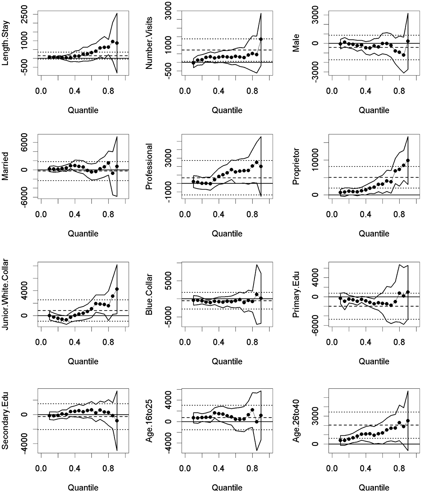
Least squares and quantile regressions estimates for total spending

The vertical distance of a solid dot from the horizontal axis can be interpreted as the impact of a one-unit change in that independent variable on the dependent variable for that chosen τ th quantile of the dependent variable holding other independent variables fixed. For example, in Figure 1, the second panel in the first row shows the relationship between the independent variable of number of visits and the dependent variable of spending on shopping. There is an increasing impact on spending on shopping with each additional number of visits for the lower 0.70 quantiles (reflecting the lower 70% of shopping spending) and a decreasing impact beyond that. Similarly, the third panel in the second row shows that visitors who are proprietors spend more than other occupation types among the top half (0.50) of the population in terms of spending on shopping. The top 10% of proprietor shoppers spent about $9,000 more than other job types visitors, which is the base level of the occupation dummy variables.

The two solid curves that envelop the solid dots are the 95% confidence band for the quantile regression coefficients. Hence, a confidence band corresponding to a solid dot of a specific τ that does not contain the solid horizontal x axis represents a quantile regression coefficient that is statistically significant at the 5% level for that particular τ. In the example of the second panel in the top row in Figure 1, the number of visits has a significant impact on shopping bills statistically only for the middle 40% of the population strata (0.3 < τ < 0.7) in which the confidence band does not envelop the solid horizontal x axis. For the rest of the population strata, the number of visits should be considered as not having an impact on shopping spending, even though the estimated coefficients are positive, since they are not significant statistically at a 5% level.

The dash horizontal line in each panel represents the least squares estimate of the conditional mean effect for the entire distribution, while the two dotted lines represent the 95% confidence interval constructed using the heteroscedasticity-robust standard error. Hence, the least squares estimate is statistically significant at the 5% level if the dotted lines do not envelop the horizontal axis. In the example from the second panel in Figure 1, the number of visits does not have a significant impact on average shopping bills because the two dotted lines envelop the horizontal axis.

In the following sections, we highlight the more significant differences that can be detected in applying the quantile regression method to data that were originally assessed by Wang (2004) using a more traditional least squares estimate approach. This will be discussed through the results shown in Tables 1 and 2, and correspondingly Figures 1 and 2, which cover spending on shopping and total spending, respectively.

Spending for Shopping

Wang (2004) found that the number of visits variable had a statistically significant positive effect on spending for shopping for the average Mainland Chinese spender in Hong Kong according to his least squares estimate. However, our least squares estimate in Table 1 concludes otherwise. This is due to the larger heteroscedasticity-robust standard error used in computing our t-test statistic. The t-test statistic was indeed significant at the 5% level if the traditional standard error was used. The quantile regression estimates reveal additional insight. This is shown graphically in the second panel in the top row of Figure 1, where number of visits has an increasingly marginal effect on shopping expenditure as we move from the first quartile of the distribution where τ = 0.25 toward the third quartile when τ reaches 0.75 but not for the bottom and top 25% shoppers (Table 1 corresponds directly to Figure 1). Therefore, each additional visit only has a higher impact on shopping expenditure among the middle 50% shoppers. While this reaffirms the previous findings that higher number of previous visits results in higher shopping spending, it is true only for the middle 50% of shoppers. The average effect, which is unduly influenced by the outliers in the upper and lower tails of the distribution, turns out to be statistically insignificant.

Table 1.

Estimated Coefficients for the Least Squares Regression (LSR) and Quantile Regressions (QR) for “Spending on Shopping”

		QR
Variables	LSR	.1	.2	.3	.4	.5	.6	.7	.8	.9
Intercept	2172.12	135.00	237.50	297.27	110.44	238.16	1505.00	1927.50*	2498.89	2838.61
Length of stay	69.93	48.33*	64.40	57.27***	52.31	36.12	26.86	62.50	22.78	217.22
Number of visits	535.25	55.00	140.70	268.73*	350.44**	389.59*	461.51*	567.50***	291.11	162.91
Male	−442.70	−31.67	−178.80	−305.27	−485.05*	−369.39	−431.05	−420.00	−54.44	514.05
Married	−391.11	−155.00	−51.40	−48.00	282.75	550.00	−58.49	−82.50	227.22	1496.84
Professional	836.23	0.00	−14.00	604.00*	904.62	764.49	1076.74*	1617.50***	2050.56*	1976.33
Proprietor	3999.21***	31.67	221.60	178.00	920.00	1358.98	2290.23*	3732.50**	6527.22***	9184.30***
Junior white collar	1055.20	10.00	−78.40	21.81	184.95	155.51	450.47	1882.50*	2913.33***	4462.41*
Blue collar	116.22	−161.67***	−297.20	−359.46	−799.56*	−1147.14	85.00	675.00	500.00	767.09
Primary/no education	−1829.08	−193.33	−341.20	−462.54*	−415.49	−713.88	−1147.09*	−1667.50	−985.56	−1746.84
Secondary/high school	−177.71	−100.00*	−108.40	89.46	516.81	614.49	492.56	400.00	68.89	553.16
Age 16 to 25	519.39	−6.67	42.60	233.12	750.00	1494.49*	714.65	647.50	1113.89	796.84
Age 26 to 40	1775.95*	100.00	310.00*	637.46**	864.51***	1204.90***	1045.70*	1182.50**	1941.11*	3427.97**

p < 0.05, **p < 0.01, ***p < 0.001.

Wang’s original least squares estimate showed that an average proprietor/owner spends about US$4,000 more than people in other job types, holding all other factors constant. An investigation of the quantile regression estimates (Table 1 and Figure 1, second row, third panel), however, reveals that proprietors/owners spend more than other job types only for the upper half of the shopping spending distribution, with the discrepancy in spending increasing as we move toward the upper tail of the distribution. The upper 10% among the proprietors/owners spend slightly more than US$9,000, which is more than double that of an average spender, when compared to the other job types.

In our final example, the average age 26 to 40 group was shown by Wang to spend slightly less than US$2,000 more than the other age group according to the least squares estimate. The quantile regression estimates (Figure 1, bottom row, third panel) also reveal that the higher spending effect of this group increases as τ increases throughout the whole spectrum of the distribution, with a couple of less than significant exceptions. The higher shopping expenditure of this particular age group might have reflected the fulfillment of a conspicuous consumption urge (spending for status) that is met by the earning ability of the group, as observed by Charles, Hurst, and Roussanov (2007) and the degree of conspicuous consumption increases drastically for the upper 30% of the cohort in the spending for shopping category.

Total Spending

Although length of stay was found to positively affect spending on meals outside hotel, spending on local transportation, and spending on hotels, in aggregate, it has no impact (Table 2 and Figure 2, first row, first panel) on total spending for an average Mainland Chinese visitor to Hong Kong, which is similar to Wang’s finding. It does, however, have a significant positive impact (about US$600) for the 0.7 to 0.8 quantile of these visitors.

Table 2.

Estimated Coefficients for the Least Squares Regression (LSR) and Quantile Regressions (QR) for “Total Spending”

		QR
Variables	LSR	.1	.2	.3	.4	.5	.6	.7	.8	.9
Intercept	4037.30*	1087.04*	1837.90***	1997.23***	–	2080.67*	3344.80*	3110.11*	–	–
Length of stay	–	56.52**	46.48***	–	–	–	–	581.14*	640.00**	–
Number of visits	717.70*	–	–	322.00*	–	–	–	–	–	–
Male	–	–	–	–	–	–	–	–	–	–
Married	–	–	–	–	–	–	–	–	–	–
Professional	–	–	–	–	–	1237.22*	1360.80*	1494.97*	2047.82*	–
Proprietor	5054.00***	–	1065.41*	–	1431.17*	2232.17*	3060.40*	3748.86*	7320.73**	9875.18**
Junior white collar	–	–	–	−705.62*	–	–	–	1864.57*	–	4260.00*
Blue collar	–	–	–	−1020.81*	–	–	–	–	–	–
Primary/no education	–	–	–	−939.19*	−869.92*	−1496.83**	–	–	–	–
Secondary/high school	–	–	–	–	–	–	–	–	–	–
Age 16 to 25	–	–	748.89*	–	1455.21*	–	–	–	–	–
Age 26 to 40	2025.90*	–	516.00*	834.81**	1083.25**	940.00*	–	1701.71*	2278.55*	–

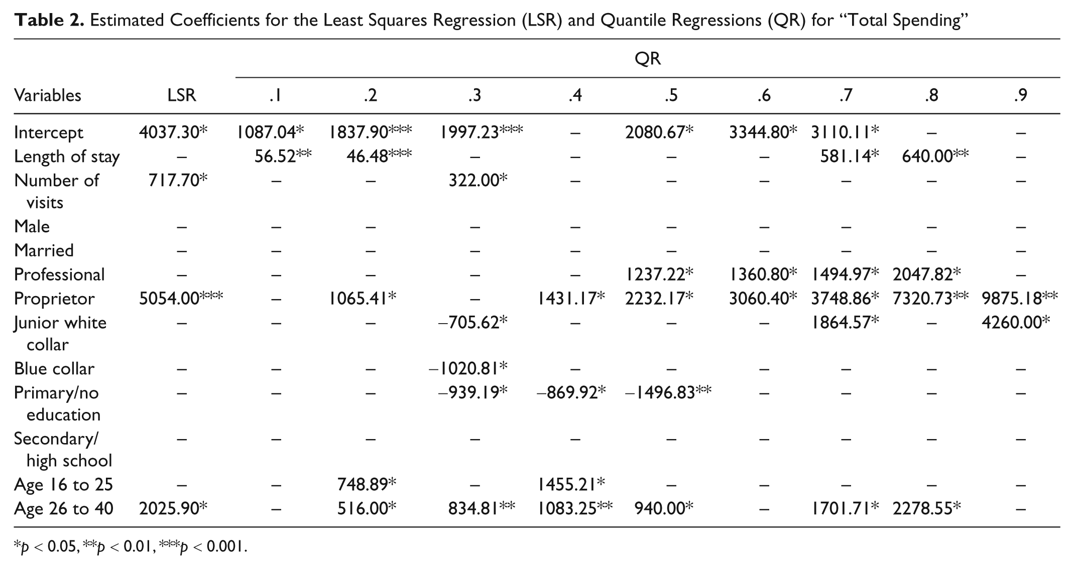
p < 0.05, **p < 0.01, ***p < 0.001.

Similar to Wang (2004), the number of visits variable (Table 2 and Figure 2, first row, second panel) has a statistically significant positive impact on total spending for an average visitor. The quantile regression estimates, however, show that this positive effect is present only for the 0.3 quantile visitors. Again, when investigating the data more carefully, we discovered that this is caused by the extremely large outliers in total spending among those who have visited Hong Kong more than three times, which biases the least squares estimate upward.

The average professionals do not have higher total spending according to the least squares estimate in Table 2 and Figure 2 (second row, second panel), a result similar to Wang’s. But they do have higher total spending (around US$1,500) among the 0.5 to 0.8 quantile cohort when compared to the base level (other job types). Wang found that the proprietors/owners (second row, third panel) have a statistically significant higher total spending than the base level on average spender and so did we. This class of tourists also spend more for almost the whole spectrum of visitors except the 0.1, 0.15, and 0.3 quantiles.

And finally, the age 26 to 40 group (fourth row, third panel) consistently spends more in total than the other age groups on average, which is contrary to Wang’s finding, and also across the whole spectrum of the distribution. The additional spending also increases as we move toward the upper tail of the distribution.

Discussions and Conclusions

Some of the least squares regression results in this study are the same as those found in Wang (2004). For the average Mainland Chinese visitor to Hong Kong, we also found that the number of visits has a significant impact on spending on meals, spending on local transportation, and total spending, as Wang found. And proprietors/owners spend on average more than the other job types on shopping and meals outside hotel.

There are also significant differences between the two studies. Contrary to Wang (2004), we cannot conclude that the number of visits has a statistically significant impact on spending for shopping for the average visitor using the heteroscedasticity-robust standard errors for the least squares estimates in light of the presence of heteroscedasticity in the models. On the contrary, we have found that the average visitor among the age 26 to 40 group has higher spending on shopping and total spending when compared to the other age groups.

More importantly, we have unveiled, through the use of quantile regressions, additional interesting effects of the covariates on the various categories of consumptions that were not revealed in Wang (2004). For example, although the number of visits is not significant in influencing spending for shopping for an average visitor, it does have a significant impact for the middle 50% of the spenders on shopping. Based on such a finding, tourism boards, cities, or any municipal entities might want to target the middle 50% of repeat visitors for shopping purposes. Higher number of visits also results in higher spending on local transportation, and this higher amount increases even more as we move from the bottom to the top of the distribution.

The quantile regression analysis also showed that the top 40% of the Mainland Chinese shoppers to Hong Kong who are proprietors/owners spend more than the other job types and the top 10% of them spend higher than four times more than the 60th percentile shoppers. Again organizations that promote shopping might want to target the higher spenders among the proprietors/owners. The middle 30% of the proprietors/owners category spend more on meals outside hotel. Proprietors/owners also spend more than other job types on hotels throughout almost the whole distribution. In aggregate, this job type has higher total spending throughout almost the whole distribution spectrum and the amount of higher spending increases as we move from the bottom toward the top of the distribution. The tourism board in Hong Kong might want to especially focus on this particular occupational group.

The age 26 to 40 group spent significantly more than the other age groups on shopping over the whole distribution, and the incremental spending is higher for the higher quantiles. This suggests that shops might want to target this age group of shoppers with their advertising campaign. This group also has higher spending on local transportation for the 0.6 to 0.8 quantiles. In aggregate, they also have higher total spending than the other age groups.

Thus, we have shown that different spending cohorts (defined by the conditional quantiles of the various spending categories) of visitors, with the same socioeconomic characteristics, length of stay, and number of visits, can have very different consumption behaviors. Understanding these differences in spending behaviors may be very useful for restaurant owners, hotel chains, transportation providers, and shopping centers when allocating their limited resources. However, as a relatively new statistical methodology, quantile regression will require considerably more testing with different data sets and case settings to both determine its applicable nuances and increase its familiarity among researchers.

We should emphasize that the findings in this study are drawn from data collected from a limited number of Mainland China’s visitors to Hong Kong. Caution should be exercised when drawing implications for visitors from other origins and to other tourist destinations, and even from other tourist markets to Hong Kong. For example, the higher spending on shopping among the proprietors/owners may be due to the higher purchasing power of the newly emerging class of self-proprietors/owners encouraged by the economic reform policy over the past 30 years in China. This high purchasing power might not exist among visitors to other tourist destinations who are proprietors/owners. Similarly, the higher shopping expenditure among the 26 to 40 age group might have reflected the exceptionally high demand for luxurious goods available only in Hong Kong fueled by high purchasing power among this group of visitors. In other tourist destinations that attract visitors from countries where luxurious goods are more readily available, we may not see the same higher shopping appetite among the same age group. Furthermore, as with all survey data, these results represent a snapshot of tourist behavior during a specific time period and under macroeconomic conditions that applied at that time.

One other method of analysis has been proposed in recent years to help destinations better distinguish big spenders from other visitors. This is the CHAID methodology, used by Legohérel and Wong (2006) and Díaz-Pérez, Bethencourt-Cejas, and Álvarez-González (2005). The CHAID methodology uses a decision tree to identify the variables with the most differences among tourist segments, with each level of the tree adding one new variable. For example, Díaz-Pérez, Bethencourt-Cejas, and Álvarez-González (2005) found nationality to be the first distinguishing factor, while the star level of the accommodation used was the second level variable. The applicable variable for the third level varied among each of the second-level groups, though visitor occupation was most significant overall. Thus, the combination of these three variables was able to explain most of the difference in tourist expenditures and could be used to develop marketing plans for different segments. The CHAID approach is effective in identifying market categories that may not be obvious in traditional market analysis and anecdotal assumptions. This complements nicely with the quantile regression technique that we have introduced in this study. The quantile regression analysis is able to discover different marginal effects that are not obvious. In particular, the quantile regression shows the significance of each independent variable on the dependent variable (expenditure) across the full spectrum of the population distribution. For example, we have shown that an additional day of stay has a higher impact on spending on meals for the upper 50% heavier spenders than it does for the lower half. The CHAID approach can then be used to help identify the heavy spenders based on their socioeconomic characteristics.

Even though quantile regression has seen a rapid rise in the past decade in its applications in fields including genetics, population biology, medicine, environmental pollution studies, political science, education, health economics, finance, demography, and Internet traffic, it still faces many challenges. For example, problems related to extreme quantile estimation, quantile regression in a seemingly unrelated regression setting and quantile regression with time series data are but a few of the rapidly evolving active research areas that could see future applications in travel research. Quantile regression, however, should not be viewed as just an alternative to the popular least squares regression to avoid potential problems like heteroscedasticity, autocorrelation, or departure from the normality assumption of the error term.

The most salient feature of using quantile regression in an analysis is to reveal the potentially much richer set of varied marginal effect of the independent variables on the dependent variables by investigating the different slope coefficient across the whole distribution of the dependent variable. We have shown that indeed the marginal effects of many of the traditional determinants of tourist spending do change over the spectrum of the population distribution. In addition, quantile regression also provides an opportunity to see differences in distributions not just differences in mean when the conditioning covariates are changed. This research illustrates how these salient features of the quantile regression technique can be exploited from the policy maker’s point of view when it comes to the better allocation of marketing resources. It also shows how they can be utilized by entrepreneurs, along the spirit of customer wallet estimation of Perlich et al. (2007), to better estimate the opportunities in marketing and sales when the paramount objective is the estimation of the potential spending by customers rather than the estimation of the average (expected) spending and, hence, provide a useful complement to existing methods.

The degree to which these insights may benefit a destination marketing organization (DMO) will vary with the competing goals and resources that are available. Policy and budgeting decisions based on tourist expenditure research is one consideration among many in the DMO mix of marketing tools. However, in instances where the manipulation of tourist expenditure patterns is identified as a significant objective in a destination marketing plan, then the more nuanced understanding that quantile regression offers of such expenditures can potentially provide a higher return on investment for limited DMO resources.

Footnotes

Acknowledgements

The authors wish to thank Dr. Donggen Wang, Department of Geography, Hong Kong Baptist University, for the use of his original data set for this study and Dr. Ken Lorek, W.A. Franke College of Business, Northern Arizona University for his suggestions and comments on earlier drafts of the paper.

The author(s) declared no potential conflicts of interest with respect to the research, authorship, and/or publication of this article.

The author(s) disclosed receipt of the following financial support for the research, authorship, and/or publication of this article:

This study was partially funded by the U.S. Fulbright Scholarship program.

References

Agarwal

V. B.

Yochum

G. R.

(1999). “Tourist Spending and Race of Visitors.” Journal of Travel Research, 38 (2): 173-76.

Barrodale

Roberts

F. D. K.

(1974). “Solution of an Overdetermined System of Equation in the l₁ norm.” Communications of the ACM, 17 (6): 319-20.

Chan

(2008). “Chinese Tourists Spend Big in Hong Kong.” Bloomberg Businessweek, July 23. http://www.businessweek.com/globalbiz/content/jul2008/gb20080723_568870.htm (accessed August 6, 2010).

Charles

K. K.

Hurs

Roussanov

(2007). “Conspicuous Consumption and Race.” http://knowledge.wharton.upenn.edu/papers/1353.pdf. (accessed May 17, 2011)

Chen

(2007). “A Finite Smoothing Algorithm for Quantile Regression.” Journal of Computational and Graphical Statistics, 16 (1): 136-64.

Chernozhukov

(2005). “Extremal Quantile Regression.” Annals of Statistics, 33 (2): 806-39.

Díaz-Pérez

F. M.

Bethencourt-Cejas

Álvarez-González

J. A. A.

(2005). “The Segmentation of Canary Island Tourism Markets by Expenditure: Implications for Tourism Policy.” Tourism Management, 26: 961-64.

English

D. B. K.

(2000). “Calculating Confidence Intervals for Regional Economic Impacts of Recreation by Bootstrapping Visitor Expenditures.” Journal of Regional Science, 40 (3): 523-39.

Frechtling

D. C.

(1994). “Assessing the Economic Impacts of Travel and Tourism—Introduction to Travel Economic Impact Estimation.” In Travel, Tourism, and Hospitality Research: A Handbook for Managers and Researchers, edited by Ritchie

J. R. B.

Goeldner

C. R.

New York: John Wiley, pp. 359-65.

10.

Hall

C. M.

Lew

A. A.

(2009). Understanding and Managing Tourism Impacts: An Integrated Approach. Oxford, UK: Routledge.

11.

Heung

V. C. S.

Cheng

(2000). “Assessing Tourists’ Satisfaction with Shopping in the Hong Kong Special Administrative Region of China.” Journal of Travel Research, 38 (4): 396-404.

12.

Hunter

D. R.

Lange

(2000). “Quantile Regression via an MM Algorithm.” Journal of Computational and Graphical Statistics, 9 (1): 60-77.

13.

Joppe

Martin

D. W.

Waalen

(2001). “Toronto’s Image as a Destination: A Comparative Importance-Satisfaction Analysis by Origin of Visitor.” Journal of Travel Research, 39 (3): 252-60.

14.

Koenker

(2009). quantreg: Quantile Regression, R package version 4.67. http://www.r-project.org. (Accessed May 17, 2011).

15.

Koenker

d’Orey

(1987). “Algorithm AS 229: Computing Regression Quantiles.” Applied Statistics, 36 (3): 383-93.

16.

Koenker

d’Orey

(1994). “Remark AS R92: A Remark on Algorithm AS 229: Computing Dual Regression Quantiles and Regression Rank Scores.” Applied Statistics, 43 (2): 410-14.

17.

Koenker

Hallock

K. F.

(2001). “Quantile Regression.” Journal of Economic Perspectives, 15 (4): 143-56.

18.

Koenker

(2005). “A Frisch-Newton Algorithm for Sparse Quantile Regression.” Acta Mathematicae Applicatae Sinica (English Series), 21 (2): 225-36.

19.

Legohérel

Wong

K. K. F.

(2006). “Market Segmentation in the Tourism Industry and Consumers’ Spending: What about Direct Expenditures?” Journal of Travel & Tourism Marketing, 20 (2): 15-30.

20.

Lehto

X. Y.

Cai

L. A.

O’Leary

J. T.

Huan

T.-C.

(2004). “Tourist Shopping Preferences and Expenditure Behaviours: The Case of the Taiwanese Outbound Market.” Journal of Vacation Marketing, 10 (4): 320-32.

21.

Lew

A. A.

McKercher

(2002). “Trip Destinations, Gateways and Itineraries: The Example of Hong Kong.” Tourism Management, 23 (6): 609-21.

22.

Mehmetoglu

(2007). “Nature-Based Tourists: The Relationship between Their Trip Expenditures and Activities.” Journal of Sustainable Tourism, 15 (2): 200-15.

23.

Mok

Iverson

T. J.

(2000). “Expenditure-Based Segmentation: Taiwanese Tourists to Guam.” Tourism Management, 21: 299-305.

24.

Narayan

P. K.

(2005). “The Structure of Tourist Expenditure in Fiji: Evidence from Unit Root Structural Break Tests.” Applied Economics, 37: 1157-61.

25.

(1996). “An Algorithm for Quantile Smoothing Splines.” Computational Statistics and Data Analysis, 22: 99-118.

26.

Lew

A. A.

(2009). “Quantile Regression Analysis of Visitor Spending: An Example of Mainland Chinese Tourists in Hong Kong.” Northern Arizona University, The W.A. Franke College of Business Working Paper Series—09-06. http://www.franke.nau.edu/Faculty/Intellectual/workingpapers/pdf/Ng_QRHKTourists.pdf (accessed February 21, 2011).

27.

J. Y.-J.

Cheng

C. K.

Lehto

X. Y.

O’Leary

J. T.

(2004). “Predictors of Tourists’ Shopping Behaviour: Examination of Socio-demographic Characteristics and Trip Typologies.” Journal of Vacation Marketing, 10 (4): 308-19.

28.

Perlich

Rosset

Lawrence

Zadrozny

(2007). “High-Quantile Modeling for Customer Wallet Estimation and Other Applications.” Proceedings of the 13th ACM SIGKDD International Conference on Knowledge Discovery and Data Mining. New York: ACM.

29.

Portnoy

Koenker

(1997). “The Gaussian Hare and the Laplacian Tortoise: Computability of Squared-Error versus Absolute-Error Estimators (with Discussions).” Statistical Sciences, 12: 279-300.

30.

R Development Core Team. (2008). R: A Language and Environment for Statistical Computing. R Foundation for Statistical Computing, Vienna, Austria. ISBN 3-900051-07-0. http://www.R-project.org. (Accessed May 17, 2011).

31.

Rosenbaum

M. S.

Spears

D. L.

(2005). “Who buys that? Who does what? Analysis of cross-cultural consumption behaviours among tourists in Hawaii.” Journal of Vacation Marketing, 11(3): 235-247.

32.

Suh

K. S.

Gartner

W. C.

(2004). “Preferences and Trip Expenditures—A Conjoint Analysis of Visitors to Seoul, Korea.” Tourism Management, 25: 127-37.

33.

Wang

(2004). “Tourist Behaviour and Repeat Visitation to Hong Kong.” Tourism Geographies, 6 (1): 99-118.

34.

Weber

(1995). “Psychographic Segmentation.” In Tourism Marketing and Management Handbook, edited by Witt

S. F.

Moutinho

Hemel Hempstead, Hertfordshire, UK: Prentice Hall, pp. 316-24.

35.

Wicks

B. E.

Schuett

M. A.

(1993). “Using Travel Brochures to Target Frequent Travellers and ‘Big-spenders.’” Journal of Travel & Tourism Marketing, 2 (2/3): 77-90.

36.

Wolff

E. N.

(2006). International Perspectives on Household Wealth. Cheltenham, UK: Edward Elgar.

37.

Wong

Law

(2003). “Differences in Shopping Satisfaction Levels: A Study of Tourists in Hong Kong.” Tourism Management, 32 (4): 401-10.

38.

Yoo

J. J.-E.

McKercher

Mena

(2004). “A Cross-Cultural Comparison of Trip Characteristics: International Visitors to Hong Kong from Mainland China and USA.” Journal of Travel & Tourism Marketing, 16 (1): 63-75.

39.

(2002). “Quantile Regression Using RJMCMC Algorithm.” Computational Statistics and Data Analysis, 40: 303-15.

40.

Stander

(2003). “Quantile Regression: Applications and Current Research Area.” Statistician, 52 (3): 331-50.