The Potential Influence of Researchers’ “Hidden” Procedure Decisions on Estimates of Visitor Spending and Economic Impact

Abstract

The potential influence of eight decisions made by researchers that are unlikely to be reported in economic impact analyses are identified and empirically tested. The data set was comprised of studies undertaken at nine state parks in Texas. Four of the decisions were categorized as being potentially relatively malignant in that they used obviously inappropriate procedures and were likely to substantially exaggerate expenditure estimates: using group weighting rather than individual weighting; omitting a measure of the extent to which visiting a park was the primary trip purpose; retaining outlier values; and aggregating different visitor segments. The four relatively benign decisions were: convenience or probability samples; managers’ or samples’ estimates of number of nonlocal visitors; treating nonresponses as missing data or as zero expenditures; and sector selection for assignment of government expenditures.

Keywords

economic impact studies visitor spending researcher decisions assumptions exaggerated estimates state parks

Economic impact is a conceptually rich phenomenon, with strong intuitive appeal, which is easily grasped by noneconomists. Economic analyses tend to reinforce this intuitive appeal because they produce quantifiable outcomes and sometimes use complex procedures, so often there is a presumption in the minds of audiences that the analyses are “scientific” and, hence, the outputs are objective and unequivocal. This is fallacious. Economic impact analysis is an inexact process, and the output numbers should be regarded as a “best guess” rather than as being inviolably accurate.

The political reality is they are usually commissioned to justify a position that their sponsors have adopted. Since there are multiple points in an economic impact analysis where underlying assumptions are made or at which alternative procedures can be adopted, there is a temptation to embrace inappropriate procedures and assumptions to generate high economic numbers that will support the sponsors’ position. It has been noted, “In some cases, the practices are the result of ignorance and are inadvertent, but far too often they are deliberate and enacted with intent to mislead and distort” (Crompton 2006, 67). That author discussed issues relating to the ethical challenges this presents and strategies for addressing them.

A review in this journal of these mischievous practices identified and discussed 10 of them (Crompton 2006). This article extends that list by identifying, discussing, and empirically testing the potential impacts of an additional eight practices on estimates of economic impact. They differ somewhat from the 10 listed in the earlier article in that those 10 are usually identifiable in reports of economic impact analyses. In contrast, the eight practices discussed in this article for the most part are “hidden.” That is, they are internal process and procedural decisions made by researchers that most lay audiences are likely to consider esoteric, arcane, and mundane, and to view with disinterest. They are frequently invisible, because they are rarely mentioned in reports. Nevertheless, they have the potential to substantially distort visitors’ expenditure and economic impact estimates. Hence, awareness of the trade-offs inherent in selecting alternative procedures is critical for any meaningful evaluation of the legitimacy of the “best guess” outcome estimates.

Methods

Data were collected at nine state parks in Texas over a four-and-a-half-month period. Surveyors intercepted visitors at the park entrance gates and campgrounds. They were convenience samples. The leader of each group of visitors was asked to report the group’s expenditures in the local community, which was defined as “within a 20-mile radius of the park.” The number of usable questionnaires obtained ranged from 390 at Daingerfield and 398 at Lake Corpus Christi, to 1,312 at Garner and 1,210 at Enchanted Rock (Tables 9 and 10).

The eight researcher decisions on which the study focused were classified as either potentially malignant or potentially benign. Potentially malignant decisions are defined by two characteristics: (1) There is an obvious correct way to proceed; and (2) if an incorrect alternative is selected, then it is likely to result in substantially distorted, and in most cases exaggerated, expenditure estimates. In contrast, for those decisions classified as being potentially relatively benign, a legitimate case can be made that supports whichever option a researcher selects; and the impact of the choice on estimates of economic impact is likely to be relatively small. In those cases, a researcher’s obligation is to describe the alternative selection and the trade-offs involved, so readers are aware of them and can make their own decision on whether or not it represents best practice.

Potentially Malignant Decisions

Four researcher decisions are classified into this category: aggregating per person expenditures by group weighting rather than by individual weighting; omitting a measure of the extent to which visiting a park was the exclusive trip purpose; retaining outlier values; and aggregating different visitor segments.

Aggregating Per-Person Expenditures by Group Weighting Rather Than by Individual Weighting

The nine economic impact studies adopted the widespread recommended practice (Crompton 2010) for collecting expenditure information of approaching the leader of a group and asking three questions;

How many days will you be visiting this park on this trip?

How many people (including yourself) are in your immediate group? (This is the number of people for whom you typically pay the bills e.g. your family or close friends)?

During the course of your visit what is the approximate amount you and other members of your immediate group will spend in each of the following categories? (Eight were listed)

Data collected from each respondent group in the samples were then aggregated and extrapolated to the parks’ annual visitation numbers.

Table 1 provides illustrative data from the leaders of three hypothetical groups: A, B, and C. Thus, for example, Leader A reported there were 4 people in his/her group; the group was in the park for 1 day, giving a total of 4 visitor days; and the group’s expenditures outside the park, but within a 20-mile radius of it, amounted to $20 per person per day.

Table 1.

Illustrative Spending Data from Three Groups.

Group	Number of Visitors in the Respondent’s Group	Number of Days in the Park	Number of Visitor Days	Total Expenditure of the Group	Per Person per Day Expenditure
A	4 people	1	4	$80	$20
B	1 person	1	1	$60	$60
C	3 people	3	9	$135	$15
Total 3 groups	8 people	5	14	$275

The average per person expenditures of the three groups (8 people) can be calculated by using either individual weighting or group weighting. Individual weighting divides the aggregate total expenditures of the groups by their aggregate visitor days:

\frac{\sum_{i = 1}^{n} E_{i}}{\sum_{i = 1}^{n} (P_{i} D_{i})} = \bar{e}

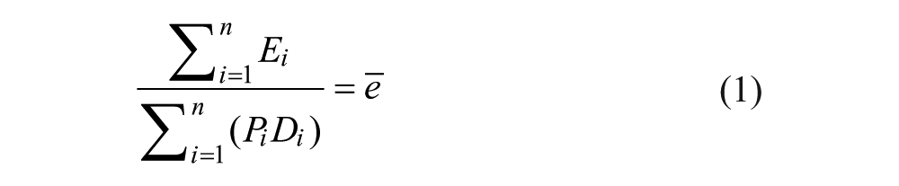
where E_i represents total expenditures by each group i, P_i is party size for each group (number of people), D_i is each group’s length of stay (number of days), n is the total number of groups or responses in the sample, and ē is the individually weighted average per person expenditures for the sample. In the example from Table 1,

($ 80 + $ 60 + $ 135) / (4 + 1 + 9) = $ 20 \times (4 / 14) + $ 60 \times (1 / 14) + $ 15 \times (9 / 14) = $ 19.64 per person per day .

If group weighting is used, then the average per person per day expenditures of each group are first calculated:

\frac{E_{i}}{P_{i} D_{i}} = e_{i}

where E_i, P_i, and D_i are defined as above and e_i represents average expenditures per person per day for group i. The average daily per person expenditures for each group are then averaged again across the sample, creating an average of an average:

\frac{\sum_{i = 1}^{n} {\dot{e}}_{i}}{n} = \dot{e}

where ė represents the group-weighted average per person expenditures for the sample. In the Table 1 example,

($ 20 + $ 60 + $ 15) / 3 = $ 20 \times (1 / 3) + $ 60 \times (1 / 3) + $ 15 \times (1 / 3) = $ 31.67 per person per day

Individual weightings give a relatively low weighting to those groups’ per person per day expenditures reporting fewer visitor days, while the per person per day expenditures for those with a greater number of visitor days are weighted relatively high. Thus, in Table 1, Group B’s per person per day expenditure is weighted 1/14, while that of Group C is weighted 9/14. In contrast, the group weightings assign a ratio of 1/3 to each group. These alternative weightings will result in systemic bias when aggregating a sample’s expenditures if a disproportionate number of groups have (1) relatively low numbers of visitor days and relatively high per person per day expenditures, or (2) relatively high number of visitor days and relatively low per person per day expenditures.

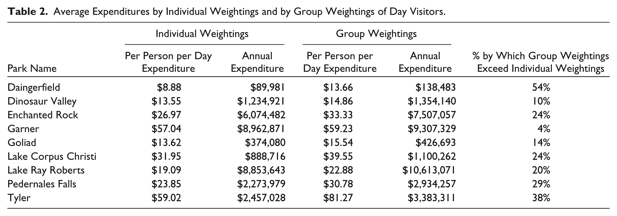
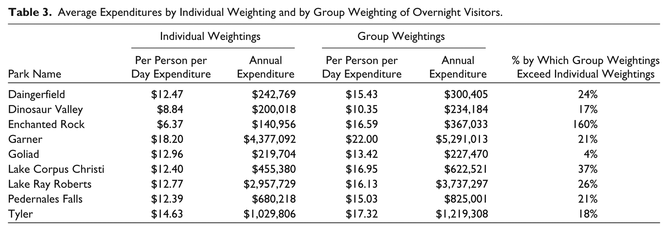
Tables 2 and 3 report the results obtained from applying each of the weighting alternatives to the data for day visitors and overnight visitors in the nine parks. In all 18 cases shown in the tables, the group weighting yielded higher dollar amounts than the individual weightings. The consistency of these results suggests systemic bias stemming from a disproportionate number of groups reporting a relatively high number of visitor days and relatively low per person per day expenditures.

Table 2.

Average Expenditures by Individual Weightings and by Group Weightings of Day Visitors.

Park Name	Individual Weightings		Group Weightings		% by Which Group Weightings Exceed Individual Weightings
Park Name	Per Person per Day Expenditure	Annual Expenditure	Per Person per Day Expenditure	Annual Expenditure	% by Which Group Weightings Exceed Individual Weightings
Daingerfield	$8.88	$89,981	$13.66	$138,483	54%
Dinosaur Valley	$13.55	$1,234,921	$14.86	$1,354,140	10%
Enchanted Rock	$26.97	$6,074,482	$33.33	$7,507,057	24%
Garner	$57.04	$8,962,871	$59.23	$9,307,329	4%
Goliad	$13.62	$374,080	$15.54	$426,693	14%
Lake Corpus Christi	$31.95	$888,716	$39.55	$1,100,262	24%
Lake Ray Roberts	$19.09	$8,853,643	$22.88	$10,613,071	20%
Pedernales Falls	$23.85	$2,273,979	$30.78	$2,934,257	29%
Tyler	$59.02	$2,457,028	$81.27	$3,383,311	38%

Table 3.

Average Expenditures by Individual Weighting and by Group Weighting of Overnight Visitors.

Park Name	Individual Weightings		Group Weightings		% by Which Group Weightings Exceed Individual Weightings
Park Name	Per Person per Day Expenditure	Annual Expenditure	Per Person per Day Expenditure	Annual Expenditure	% by Which Group Weightings Exceed Individual Weightings
Daingerfield	$12.47	$242,769	$15.43	$300,405	24%
Dinosaur Valley	$8.84	$200,018	$10.35	$234,184	17%
Enchanted Rock	$6.37	$140,956	$16.59	$367,033	160%
Garner	$18.20	$4,377,092	$22.00	$5,291,013	21%
Goliad	$12.96	$219,704	$13.42	$227,470	4%
Lake Corpus Christi	$12.40	$455,380	$16.95	$622,521	37%
Lake Ray Roberts	$12.77	$2,957,729	$16.13	$3,737,297	26%
Pedernales Falls	$12.39	$680,218	$15.03	$825,001	21%
Tyler	$14.63	$1,029,806	$17.32	$1,219,308	18%

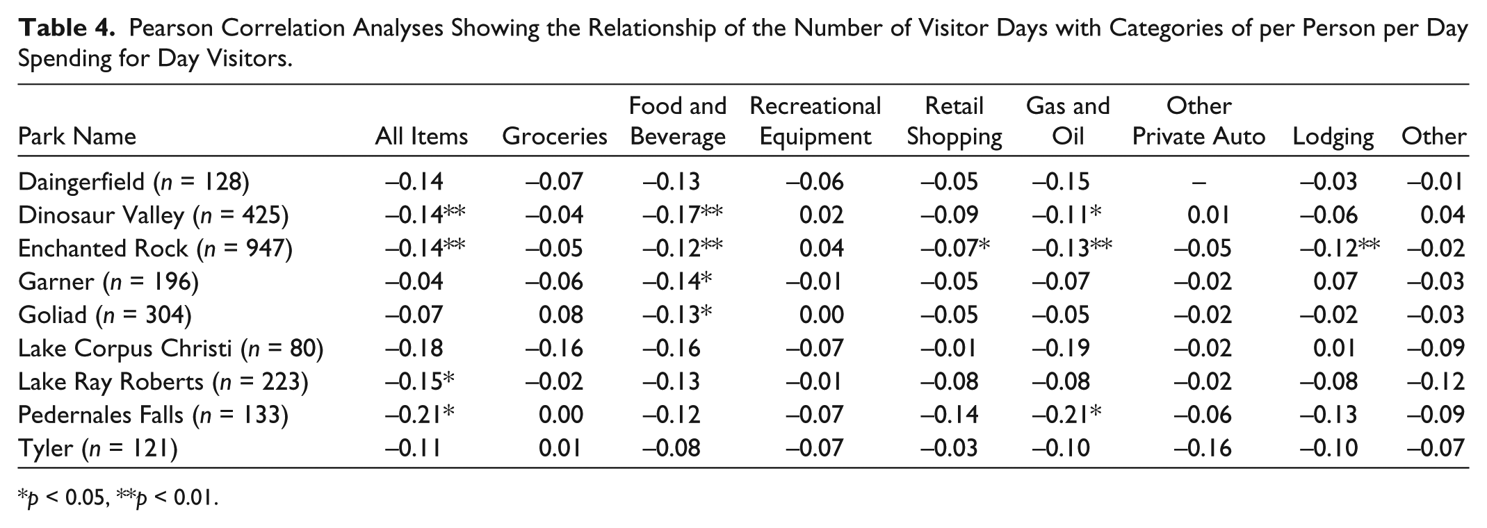
Empirical support for this explanation was provided by the correlation analyses reported in Tables 4 and 5. When numbers of visitor days for day visitors and overnight visitors were correlated with per person per day expenditures in each category, the relationship was consistently negative indicating that as visitor days per group increased, per person per day expenditure declined. This suggests there are economies of scale both as the group size increases and as the length of stay increases. As the costs of items purchased in association with a park visit are spread across more visitor days, the average per person per day expenditure is reduced.

Table 4.

Pearson Correlation Analyses Showing the Relationship of the Number of Visitor Days with Categories of per Person per Day Spending for Day Visitors.

Park Name	All Items	Groceries	Food and Beverage	Recreational Equipment	Retail Shopping	Gas and Oil	Other Private Auto	Lodging	Other
Daingerfield (n = 128)	−0.14	−0.07	−0.13	−0.06	−0.05	−0.15	–	−0.03	−0.01
Dinosaur Valley (n = 425)	−0.14**	−0.04	−0.17**	0.02	−0.09	−0.11*	0.01	−0.06	0.04
Enchanted Rock (n = 947)	−0.14**	−0.05	−0.12**	0.04	−0.07*	−0.13**	−0.05	−0.12**	−0.02
Garner (n = 196)	−0.04	−0.06	−0.14*	−0.01	−0.05	−0.07	−0.02	0.07	−0.03
Goliad (n = 304)	−0.07	0.08	−0.13*	0.00	−0.05	−0.05	−0.02	−0.02	−0.03
Lake Corpus Christi (n = 80)	−0.18	−0.16	−0.16	−0.07	−0.01	−0.19	−0.02	0.01	−0.09
Lake Ray Roberts (n = 223)	−0.15*	−0.02	−0.13	−0.01	−0.08	−0.08	−0.02	−0.08	−0.12
Pedernales Falls (n = 133)	−0.21*	0.00	−0.12	−0.07	−0.14	−0.21*	−0.06	−0.13	−0.09
Tyler (n = 121)	−0.11	0.01	−0.08	−0.07	−0.03	−0.10	−0.16	−0.10	−0.07

p < 0.05, **p < 0.01.

Table 5.

Pearson Correlation Analyses Showing the Relationship of the Number of Visitor Days with Categories of per Person per Day Spending for Overnight Visitors.

Park Name	All Items	Groceries	Food and Beverage	Recreational Equipment	Retail Shopping	Gas and Oil	Other Private Auto	Lodging	Other
Daingerfield (n = 254)	−0.17**	−0.15*	−0.02	−0.04	−0.08	−0.16*	−0.05	−0.02	0.02
Dinosaur Valley (n = 81)	−0.22*	−0.26*	−0.18	0.05	−0.05	−0.14	0.14	.	0.09
Enchanted Rock (n = 239)	−0.15*	−0.11	−0.12	−0.05	−0.07	−0.17**	−0.04	−0.06	−0.03
Garner (n = 1,090)	−0.15**	−0.14**	−0.12**	−0.06*	−0.05	−0.17**	−0.02	−0.03	−0.04
Goliad (n = 140)	−0.05	0.09	0.03	0.01	−0.02	−0.07	0.06	−0.14	−0.08
Lake Corpus Christi (n = 310)	−0.36**	−0.28**	−0.21**	−0.14*	−0.11	−0.36**	−0.05	−0.08	−0.02
Lake Ray Roberts (n = 276)	−0.22**	−0.16**	−0.15*	−0.11	−0.08	−0.15*	−0.02	−0.10	0.00
Pedernales Falls (n = 361)	−0.15**	−0.13*	−0.06	−0.06	−0.05	−0.18**	0.12*	0.01	−0.04
Tyler (n = 326)	−0.16**	−0.09	−0.12*	−0.10	−0.02	−0.18**	−0.02	−0.03	−0.04

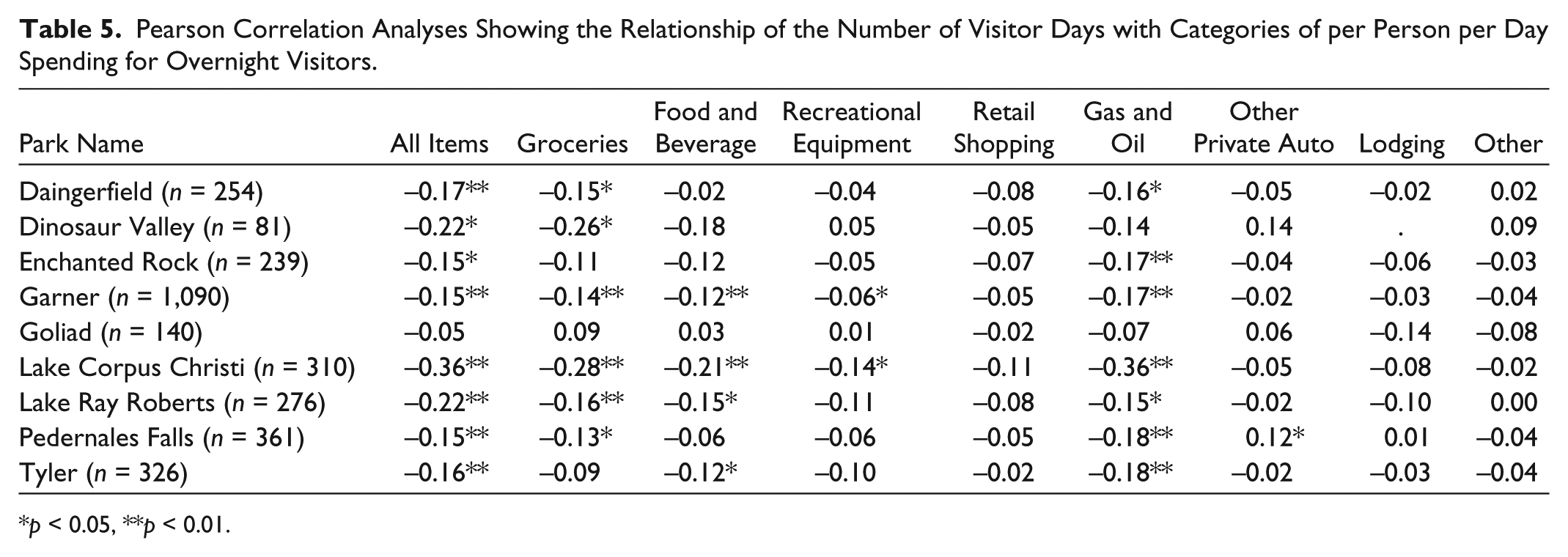
p < 0.05, **p < 0.01.

Analyses of these data suggest that using group weightings, rather than individual weightings, is likely to produce substantially exaggerated average expenditures. It is mathematically possible to obtain smaller group-weighted expenditures, but in practice it is a rare occurrence for the reasons stated above. Indeed, perhaps the only situation in which they are appropriate is when the population’s unit of analysis is number of groups. If Texas State Parks measured their annual attendance by number of groups (rather than by visitors or visitor days), then aggregating samples by group weightings would be consistent with that unit of analysis and representative of that measure. Examples may be parking lot counts or boat launch data, which are group measures.

Omitting a Measure of the Extent to Which Visiting a Park Was the Primary Trip Purpose

For more than two decades, the importance of identifying “time-switchers” and “casuals” and removing them from economic impact analyses has been recognized, and the potentially egregious errors that may occur if this is not done has been demonstrated (Crompton and McKay 1994). Time-switchers are those who were planning a trip to an area, but changed the timing of their visit to coincide with a particular event: “Their spending cannot be attributed to the event, because it would have been made without the event, albeit at a different time of the year” (Crompton 1995, 27). In the context of state parks, time-switchers are not a prominent concern because, for the most part, the parks do not host events.

Casuals are visitors who are already in the area, attracted by other elements (e.g., business travel or visiting either family or friends), who elected to visit the state park instead of doing something else (Crompton and McKay 1994). Their economic impact should not be attributable to the park, because if they had not visited it, the likely scenario is they would have spent a similar amount of money elsewhere in the area. Typically, casuals are identified and screened out of an economic impact study by asking:

Would you have come to this area if the state park was not here?

If yes, Did you stay longer in the area than you would have done if the state park was not here?

If yes, how many days longer?

The first question in this sequence requires a dichotomous yes or no response. However, the answer for many is unlikely to be absolute; rather it is likely to be qualified. Thus, among those responding that they would have come to the area if the park was not there, there are likely to be some for whom, even though it was not a primary driver, it provided an additional increment of benefit that was influential in their decision to make the trip. Similarly, among those indicating they would not have visited the area if the park was not there, there are likely to be some for whom there were other complementary reasons that contributed to the decision to make the trip.

These scenarios suggest two modifications to the conventional practice for screening time-switchers and casuals. First, a scale rather than dichotomous categories is more appropriate for measuring a park’s influence on the decision to visit an area. Second, in addition to discounting the expenditures of those two groups, the complementary role to the state parks of other attractions in the area should be measured so park visitor expenditures can be discounted to reflect it. The latter modification has not been addressed in the economic impact literature to this point.

In his pioneering model of a tourism system, Gunn (1972) noted that attractions drive tourists to an area. A corollary of his conceptualization was that as the number and magnitude of attractions increased, both the number of visitors and their length of stay in an area were likely to increase. This corollary was analogous to the theory of cumulative attraction that was articulated in the early literature on retailing: “A given number of stores dealing in the same merchandise will do more business if they are located adjacent or in proximity to each other than if they are widely scattered” (Nelson 1958, 58).When retail outlets of a similar nature are clustered together, their attraction power tends to increase. In an early article addressing the notion of cumulative attraction, Wall (1978) noted,

Recreation sites do not exist in isolation. They are found within a context of competing and complementary facilities. . . . Patronage of any particular recreation site and the activities undertaken there only partially reflect the intrinsic characteristics of the site. Patrons are also influenced by opportunities available at other sites. (35)

In recent years, the definition of a destination has evolved from being static and politically and geographically bounded to having “variable geometry” (Beritelli, Bieger, and Laesser 2014). This organic conceptualization reflects the dynamic preferences of visitors and tourism suppliers’ responses to them within and around a geographical area. Conceptualizing destinations as industrial districts, clusters, networks, systems, or social constructs (Pearce 2014) recognizes that individuals are likely to be seeking a diverse array of experiences and benefits from a tourism encounter. Further, the experiences sought by members within a social group may be different. Both of these situations suggest it is more likely people will visit an area with multiple attractions rather than an area with few attractions. Subsequently, several studies have empirically verified the theory of cumulative attraction in tourism (Crompton and Gitelson 1979; Mings and McHugh 1992; Kim and Fesenmaier 1990; Hunt and Crompton 2008; Lue, Crompton, and Stewart 1996; Lue, Crompton, and Fesenmaier 1993).

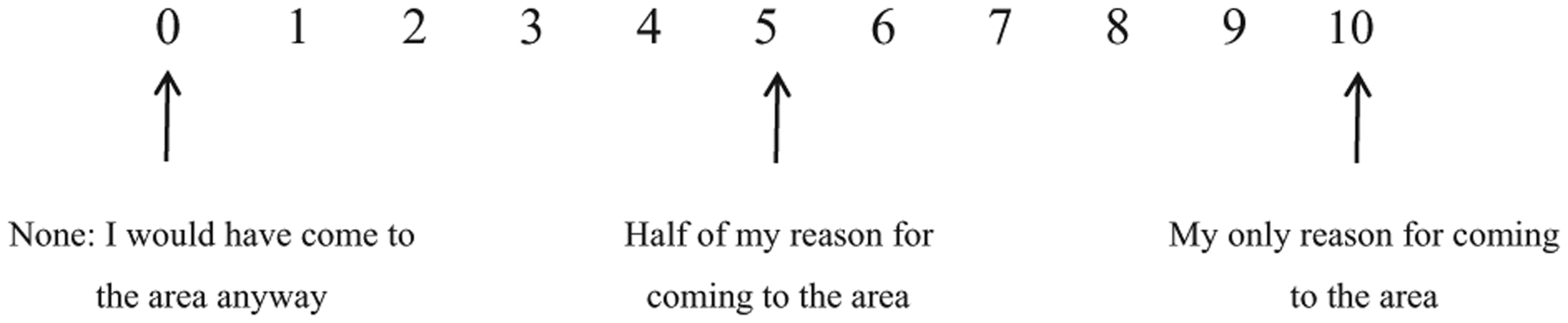
To capture both the relative attraction influence of a park within the broader context of the area’s cumulative attractions, and the appropriate discount for those who qualified as casuals (and time-switchers if there were any), the survey instrument incorporated the following scale question:

Circle the number below that best represents the extent to which visiting the park was the primary purpose of your trip to this area. A 0 indicates the park had no influence and you would have come anyway, while a 10 indicates that the park is your only reason for visiting the area on this trip.

The response to the above question was considered a “proportionality measure” with values between 0% and 100% (Tyrrell and Johnston 2001). Each respondent’s expenditures were multiplied by their proportionality measure. In the example above, the score of five indicated the park was 50% of the reason for the trip. Thus, the respondents’ expenditures would be multiplied by 50%. If the respondent spent $100, only $50 would be attributed to the park while the remaining $50 would be attributed to other reasons for visiting the area.

It is recognized that respondents’ estimates of proportionality are subject to error. However, it seems probable that resultant estimates of direct expenditures will be more accurate than the alternative strategy of using inappropriate dichotomous questions to screen casuals and time-switchers, and disregarding the influence of other attractions that may have contributed to the decision to visit the area.

The data in Table 6 show the parks tended to be the primary reason for overnight visitors coming to the area. While most of these visitors stayed in the park, some probably used it as a base to explore the area: “Tourists adopting this travel route stay at the primary destination throughout their vacation, and use it as a ‘base camp’ from which to visit places within the area” (Lue, Crompton, and Fesenmaier 1993, 295). Thus, at none of the nine parks did the proportionality measure reduce the expenditure estimates by more than 19%.

Table 6.

Expenditures That Include and Exclude a Measure of the Extent to Which Visiting a Park Was the Primary Trip Purpose of Overnight Visitors.

Park Name	Include Proportionality of Spending		Exclude Proportionality of Spending		% by Which the Exclusive Calculations Exceed Inclusive Calculations
Park Name	Per Person per Day Expenditure	Annual Expenditure	Per Person per Day Expenditure	Annual Expenditure
Daingerfield	$12.47	$242,769	$13.03	$253,658	4%
Dinosaur Valley	$8.84	$200,018	$10.03	$227,076	14%
Enchanted Rock	$6.37	$140,956	$7.56	$167,310	19%
Garner	$18.20	$4,377,092	$19.58	$4,709,476	8%
Goliad	$12.96	$219,704	$14.62	$247,723	13%
Lake Corpus Christi	$12.40	$455,380	$13.72	$504,206	11%
Lake Ray Roberts	$12.77	$2,957,729	$14.10	$3,266,906	10%
Pedernales Falls	$12.39	$680,218	$14.23	$781,319	15%
Tyler	$14.63	$1,029,806	$16.05	$1,129,621	10%

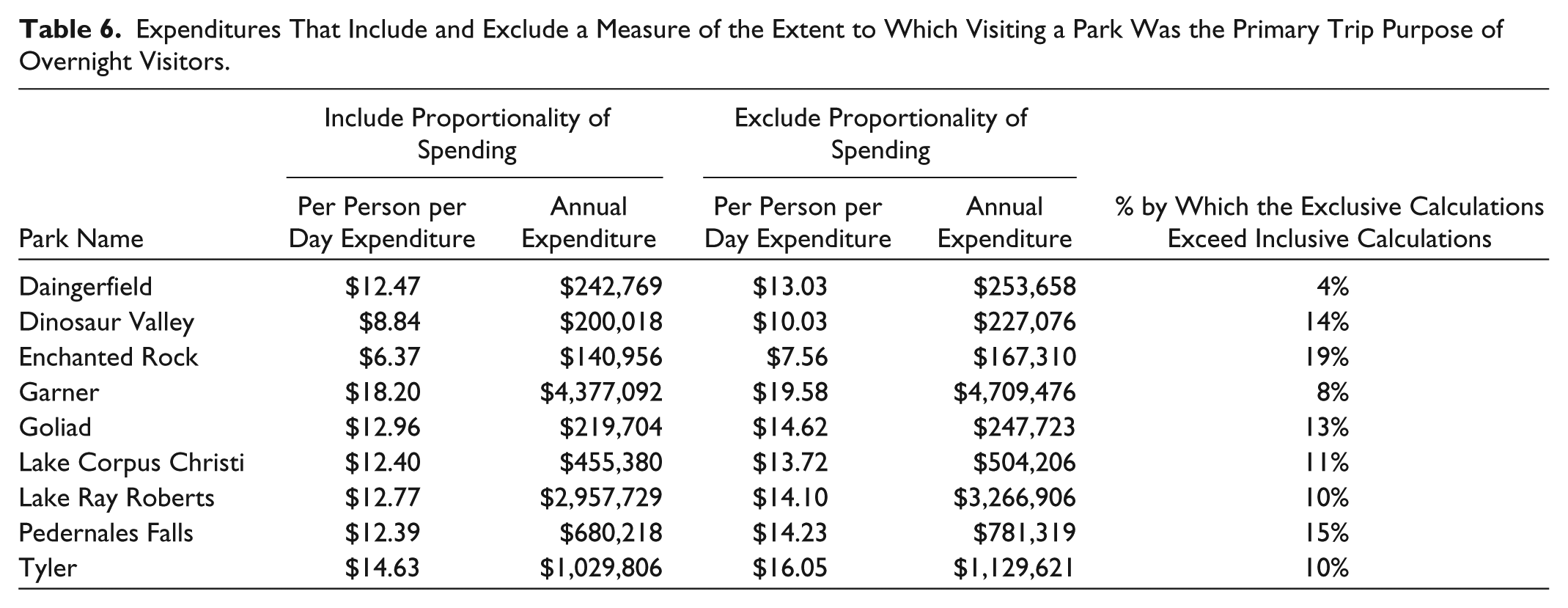
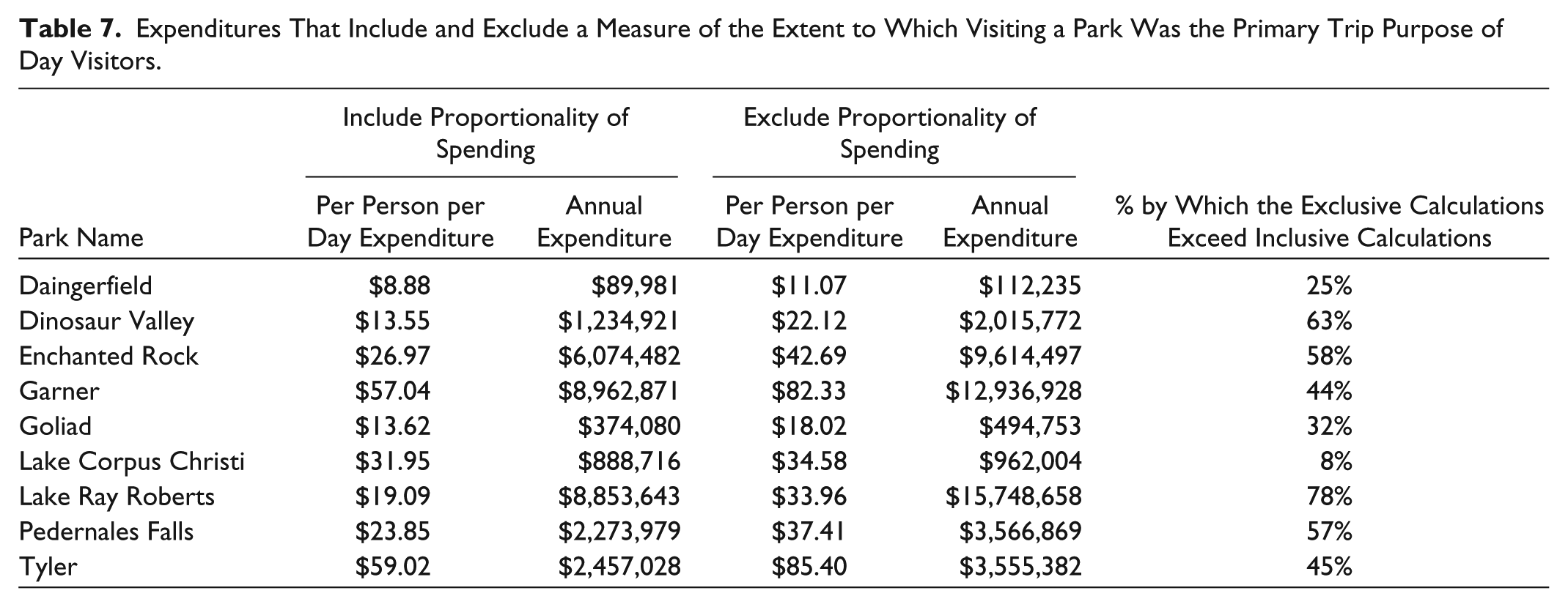
Table 7 shows that among day visitors, most of the parks were much less influential in decisions to visit the area. At Lake Ray Roberts, for example, when the proportionality measure was applied, the estimate of day visitor expenditures was dramatically reduced from $15.7 million to $8.9 million. It appears that many day visitors to Lake Ray Roberts, Dinosaur Valley, Enchanted Rock, Pedernales Falls, and Garner were either casuals or were persuaded to visit the area by the presence of multiple attractions, rather than only the park.

Table 7.

Expenditures That Include and Exclude a Measure of the Extent to Which Visiting a Park Was the Primary Trip Purpose of Day Visitors.

Park Name	Include Proportionality of Spending		Exclude Proportionality of Spending		% by Which the Exclusive Calculations Exceed Inclusive Calculations
Park Name	Per Person per Day Expenditure	Annual Expenditure	Per Person per Day Expenditure	Annual Expenditure
Daingerfield	$8.88	$89,981	$11.07	$112,235	25%
Dinosaur Valley	$13.55	$1,234,921	$22.12	$2,015,772	63%
Enchanted Rock	$26.97	$6,074,482	$42.69	$9,614,497	58%
Garner	$57.04	$8,962,871	$82.33	$12,936,928	44%
Goliad	$13.62	$374,080	$18.02	$494,753	32%
Lake Corpus Christi	$31.95	$888,716	$34.58	$962,004	8%
Lake Ray Roberts	$19.09	$8,853,643	$33.96	$15,748,658	78%
Pedernales Falls	$23.85	$2,273,979	$37.41	$3,566,869	57%
Tyler	$59.02	$2,457,028	$85.40	$3,555,382	45%

The survey instrument used at the nine parks did not include the three question sequence relating to casuals. Thus, it was not possible to compare responses on the proportionality scale with that approach. However, both measures were included in another economic impact study which the authors undertook during the same time period at Blue Hole Regional Park in Texas. The results are shown in Table 8.

Table 8.

Comparison of the Annual Expenditures of Nonlocal Visitors to Blue Hole Regional Park Excluding a Trip Purpose Measure, with the Proportionality Measure, and a Casuals Measure.

Items	Without a Trip Purpose Measure	With a Trip Purpose Measure	With a Casuals Measure
Admission Fees	$301,066	$255,520	$247,290
Groceries	$43,574	$32,741	$27,850
Restaurants and Bars	$156,408	$109,622	$85,787
Recreational Equipment	$12,861	$9,755	$9,318
Retail Shopping	$36,130	$27,639	$22,555
Gas and Oil	$17,382	$13,722	$12,402
Lodging Expenses	$961,522	$510,192	$100,205
Other Expenses	$12,666	$12,666	$12,260
Total	$1,541,609	$971,857	$517,667

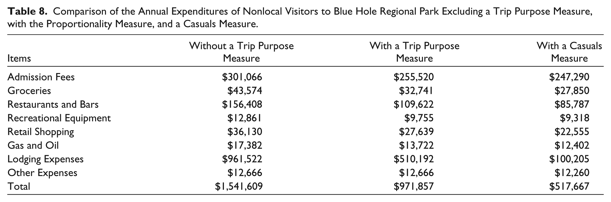
All those surveyed at Blue Hole Park were day visitors. Consistent with the findings reported in Table 7, excluding the proportionality measure resulted in a 59% increase in the estimate of annual economic impact. However, the proportionality measure was 88% greater than the casuals measure, suggesting that for many who defined themselves as casuals, the park did provide extra increments of benefit that were instrumental in their decision to visit the area. If the casuals measure had been used rather than the proportionality measure, then the economic impact estimate of the Blue Hole Park would have been substantially underestimated.

Retaining Outlier Values

When estimates derived from relatively small samples are extrapolated to relatively large populations, sampling “accidents” can lead to substantial misrepresentation. By the luck of the draw, a grossly unrepresentative case that is not consistent with typical spending behavior associated with visiting a state park may be included in a sample. Such cases may accurately reflect extraordinary purchases made by a sample respondent. However, “contaminant” errors may occur, for example, a misplaced decimal point may result in $10.00 being entered as $1000 (Stynes and White 2006). Unfortunately, there also may be deliberate acts of “sabotage.” That is, there are some warped people who derive a peculiar satisfaction from purposefully responding to survey questions with outrageous answers, so as to deliberately sabotage and distort the study’s findings. Irrespective of the motive, when collecting direct expenditure data, a very small number of unreasonably large extreme values can greatly exaggerate a population estimate.

In addition to the “accident” and “vandalism” scenarios, it has been suggested there is a strong conceptual argument for not attributing large one-off expenditures (such as the horse trailer purchase described below) to the presence of a specific park. The thinking is that these are not variable costs associated with a particular trip. Rather they are fixed costs, incurred only irregularly, which will be used on multiple trips (Gratton and Taylor 1995). Hence, expenditures on them should be spread over all the purchaser’s trips:

Generally, if visitors purchase durable “big-ticket” items such as boats, recreational vehicles, televisions or whatever, they are excluded from the analysis because these purchases are likely to be used on many trips rather than being exclusively associated with a specific trip to a facility or area. (Crompton 2010, 34)¹

Despite these concerns, many economic impact studies do not omit outlier expenditures (e.g., AHRRC 2009; Dougherty 2010; Fly et al. 2011). To evaluate the potential impacts of outlier expenditures in the nine parks’ samples, the highest 1% and lowest 1% of per person per day expenditures were removed from the analyses. Thus, among park samples with fewer than 150 respondents, two outliers (one high and one low) were omitted; four were omitted in samples ranging from 151 to 250, and so on. The procedure for removing the outliers, using overnight visits to Pedernales Falls as an illustration, is described in the appendix. The impact invariably will be greater upon the highest 1%, since in all nine parks multiple groups reported zero expenditures. Thus, exclusion of the lowest 1% had minimal impact on the average expenditures. Nonetheless, they were omitted so the procedure was balanced.²

The data in Tables 9 and 10 show that failure to incorporate the outlier procedure had a substantive impact on nearly all the 18 populations. In three cases (16.7%), it was extraordinary, resulting in an increase in the expenditure estimates among day visitors of 496% at Pedernales Falls and 376% at Lake Ray Roberts, while among overnight visitors omitting the lowest 1% and the highest 1% of outliers reduced the direct expenditures estimate at Garner from $8.9 million to $4.4 million.

Table 9.

Analyses of Data That Omitted Outliers and Did Not Omit Outliers for Day Visitors.

Park Name	Omitted Outliers				Outliers Not Omitted				% by Which Analyses That Did Not Omit Outliers Exceeded Analyses That Omitted Outliers
Park Name	Sample Size (N)	Visitor Days	Per Person per Day Expenditure	Annual Expenditure	Sample Size (N)	Visitor Days	Per Person per Day Expenditure	Annual Expenditure
Daingerfield	128	689	$8.88	$89,981	130	697	$9.56	$96,947	8%
Dinosaur Valley	425	1,409	$13.55	$1,234,921	433	1,425	$14.50	$1,321,144	7%
Enchanted Rock	947	3,198	$26.97	$6,074,482	967	3,245	$31.40	$7,071,108	16%
Garner	196	932	$57.04	$8,962,871	200	950	$61.20	$9,616,730	7%
Goliad	304	1,081	$13.62	$374,080	310	1,093	$15.19	$417,252	12%
Lake Corpus Christi	80	353	$31.95	$888,716	82	361	$35.14	$977,519	10%
Lake Ray Roberts	223	558	$19.09	$8,853,643	227	564	$90.95	$42,183,987	376%
Pedernales Falls	133	380	$23.85	$2,273,979	135	382	$142.23	$13,561,087	496%
Tyler	121	439	$59.02	$2,457,028	123	441	$60.45	$2,516,685	2%

Table 10.

Analyses of Data That Omitted Outliers and Did Not Omit Outliers for Overnight Visitors.

Park Name	Omitted Outliers				Outliers Not Omitted				% by Which Analyses That Did Not Omit Outliers Exceed Analyses That Omitted Outliers
Park Name	Sample Size (n)	Visitor Days	Per Person per Day Expenditure	Annual Expenditure	Sample Size (n)	Visitor Days	Per Person per Day Expenditure	Annual Expenditure
Daingerfield	254	3,596	$12.47	$242,769	260	3,664	$13.47	$262,116	8%
Dinosaur Valley	81	717	$8.84	$200,018	83	729	$9.87	$223,428	12%
Enchanted Rock	239	5,205	$6.37	$140,956	243	5,221	$6.80	$150,419	7%
Garner	1,090	18,963	$18.20	$4,377,092	1,112	19,180	$37.21	$8,950,657	104%
Goliad	140	1,569	$12.96	$219,704	142	1,585	$13.20	$223,688	2%
Lake Corpus Christi	310	4,241	$12.40	$455,380	316	4,271	$12.73	$467,733	3%
Lake Ray Roberts	276	4,293	$12.77	$2,957,729	282	4,329	$13.15	$3,035,231	3%
Pedernales Falls	361	4,119	$12.39	$680,218	369	4,174	$13.03	$715,425	5%
Tyler	326	4,008	$14.63	$1,029,806	332	4,048	$15.36	$1,081,162	5%

At Lake Ray Roberts, the huge distortion was attributable to a single individual who reported he was alone, stayed in the park for one day, and recorded a 10 on the trip purpose scale indicating visiting the park was his only reason for coming to the area. However, while he was in the area, he decided to purchase a new horse trailer for $39,810. Similarly, at Pedernales Falls, a single individual who reported he was alone, stayed at the park for one day, and recorded a 9 on the trip purpose scale, indicated he purchased a recreational vehicle while in the area for $50,000. Each of these single cases massively skewed the sample averages. Clearly, it was inappropriate to include them. These results vividly confirm that omitting outliers at the (say) highest, and lowest, 1% level adopted here should be a fundamental procedure in estimating average direct expenditures.

Aggregating Different Visitor Segments

It is recommended that if there are visitor groups that can be differentiated “and their economic contributions are to be estimated, then each of them needs to be sampled, because it is likely that different groups will report different expenditure amounts and patterns” (Crompton 2010, 32). In this study, it seemed likely that day and overnight visitors would have different expenditure patterns. Thus, to reduce variances both were sampled and the data used to separately calculate the expenditures of each group. Others, who have undertaken economic impact studies of state parks, however, have elected to aggregate expenditures, rather than to disaggregate them (e.g., Greenwood and Vick 2008; AHRRC 2009).

The first columns of Tables 2 and 3 confirmed the initial proposition that the per person per day average expenditures of the two groups were likely to be different. In eight of the nine parks (Daingerfield was the exception), expenditures by overnight visitors were smaller than those of day visitors, and in most cases the differences were substantial (e.g., 323% at Enchanted Rock and 213% at Garner). This is because overnight groups remain in the parks for a longer period of time, which translates into more visitor days and results in economies of scale.

To gain insight into differences that may emerge from adopting an aggregate or disaggregated approach, total visitor expenditures were calculated using both strategies so comparisons could be made. The results in Table 11 show that visitor expenditures at all the parks except Daingerfield were lower when the two segments were aggregated. In three cases, (Daingerfield, Dinosaur Valley, and Goliad), the differences were relatively small, but at the other six parks they were substantial.

Table 11.

Estimated Annual Expenditure of Visitors at Nine State Parks Using Aggregated and Disaggregated Approaches.

Park Name	Disaggregated Approach	Aggregated Approach	% Difference
Daingerfield	$332,750	$352,088	5.8%
Dinosaur Valley	$1,434,940	$1,360,772	−5.2%
Enchanted Rock	$6,215,438	$1,700,990	−72.6%
Garner	$13,339,963	$7,959,952	−40.3%
Goliad	$593,784	$587,634	−1.0%
Lake Corpus Christi	$1,344,096	$897,188	−33.2%
Lake Ray Roberts	$11,811,373	$9,354,029	−20.8%
Pedernales Falls	$2,954,198	$2,007,061	−32.1%
Tyler	$3,486,834	$1,665,341	−52.2%

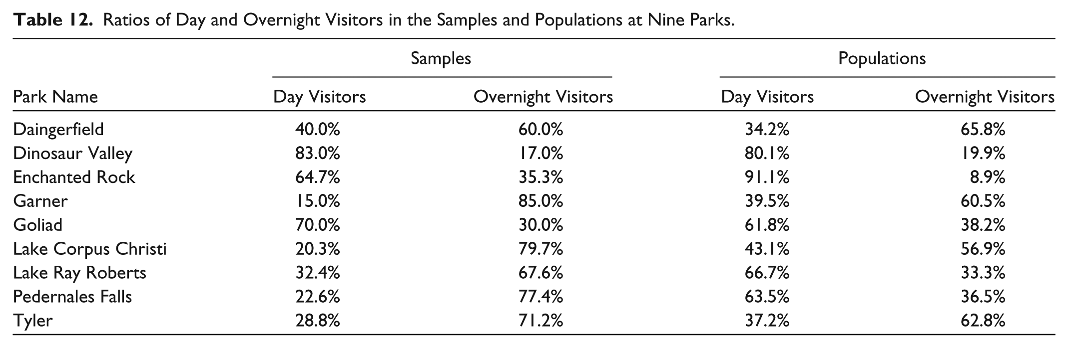
Reasons for the disparities are apparent in Table 12, which reports the ratios of day and overnight visitors in both the samples and the populations. In cases where the sample ratios are different from those in the parks’ populations, the estimates of visitor spending will be different. This will be amplified in contexts where the direct spending in a park by each of the two groups (Tables 2 and 3) is substantially different (e.g., Enchanted Rock, Garner, and Tyler). The aggregation approach assumes the sample ratios reflect those of the population. Table 12 suggests this is not a reasonable assumption and in an unacceptable number of cases is likely to result in expenditure estimates that are substantially misleading.

Table 12.

Ratios of Day and Overnight Visitors in the Samples and Populations at Nine Parks.

Park Name	Samples		Populations
Park Name	Day Visitors	Overnight Visitors	Day Visitors	Overnight Visitors
Daingerfield	40.0%	60.0%	34.2%	65.8%
Dinosaur Valley	83.0%	17.0%	80.1%	19.9%
Enchanted Rock	64.7%	35.3%	91.1%	8.9%
Garner	15.0%	85.0%	39.5%	60.5%
Goliad	70.0%	30.0%	61.8%	38.2%
Lake Corpus Christi	20.3%	79.7%	43.1%	56.9%
Lake Ray Roberts	32.4%	67.6%	66.7%	33.3%
Pedernales Falls	22.6%	77.4%	63.5%	36.5%
Tyler	28.8%	71.2%	37.2%	62.8%

The Cumulative Impact of Malignant Decisions

The aggregation of visitor segments resulted in inappropriately reduced estimates of visitor expenditures, but in each of the first three researcher decisions discussed in this section selection of the inappropriate alternative led to exaggerated estimates. The hyperbole associated with malignancy grows exponentially when all of these erroneous alternative procedures are used.

Their additive effect is shown in Table 13. The differences are sufficiently large that they grossly mislead, rather than inform. The table illustrates the potentially egregious estimates that can emerge, with the expenditures at Lake Ray Roberts and Pedernales Falls rising to $105.1 million and $40.7 million, respectively, instead of $11.8 million and $2.9 million, which were the estimates when the appropriate alternatives were selected. At only one of the nine parks was the exaggerated estimate as low as 50%.

Table 13.

The Cumulative Impact of Three Erroneous Decisions on Both Day and Overnight Visitors’ Expenditures.

Park Name	Appropriate Decisions		Inappropriate Decisions		% by Which Inappropriate Decisions Exceed Appropriate Decisions
Park Name	Per Person per Day Expenditures	Annual Expenditures	Per Person per Day Expenditures	Annual Expenditures
Daingerfield	$11.24	$332,750	$19.03	$933,897	65%
Dinosaur Valley	$12.61	$1,434,940	$23.70	$2,696,704	88%
Enchanted Rock	$25.13	$6,215,438	$60.73	$15,020,018	142%
Garner	$33.55	$13,339,963	$77.76	$30,923,109	132%
Goliad	$13.37	$593,784	$21.27	$944,367	59%
Lake Corpus Christi	$20.82	$1,344,096	$31.31	$2,021,173	50%
Lake Ray Roberts	$16.98	$11,811,373	$151.19	$105,141,261	790%
Pedernales Falls	$19.66	$2,954,198	$270.83	$40,689,600	1,277%
Tyler	$31.13	$3,486,834	$57.31	$6,419,026	84%

Potentially Relatively Benign Decisions

Four researcher decisions in this category were empirically investigated: convenience or probability samples; managers’ estimates or samples’ estimates of number of nonlocal day visitors; treating nonresponses as missing data or as zero expenditures; and sector selection for assignment of government expenditures.

In contrast to decisions classified as potentially malignant, researchers have discretion in these benign decisions, since legitimate arguments can be offered to support whichever alternative is selected. Nevertheless, the selections do have a differential impact on the magnitude of visitor expenditures and economic impacts, so they should be explicitly specified in a report and the trade-offs described.

Convenience or Probability Samples?

In a perfect world, a probability sample (i.e., random, stratified or clustered) would always be preferred to a convenience sample. However, in on-site field contexts, probability sampling is both difficult and costly. Given that resources are limited, the trade-off decision confronted in the study was probably fairly typical: Should available resources be invested in probability samples at a small number of parks, or in convenience samples at a substantially larger number of parks?

The decision will be strongly influenced by the degree of homogeneity of the population for as Babbie (1995) noted, if the population is homogeneous in every dimension then “one case would be sufficient as a sample to study characteristics of the whole population” (190). In the context of this article, homogeneity is operationalized as those who are engaged in the same activity in the same resource setting (Becker, Dottavio, and Mengak 1987).

There is evidence suggesting that state park visitors are relatively homogenous in terms of their interests and behaviors. In these situations, it has been suggested that low response rates to surveys and use of convenience samples may be acceptable (Becker, Dottavio, and Mengak 1987; Hammit and McDonald 1982; Becker and Iliff 1983). For example, Becker, Dottavio, and Mengak (1987) concluded; “Based upon the previously cited studies and our results, we believe engagement in a specific recreation activity at a specific location may be sufficient criterion to anticipate a homogenous population” (139).

An analysis of earlier Texas state park studies offered some support for their populations being relatively homogenous. Data were collected on 88 interest/behavioral variables from three previous studies (Crompton and Tian-Cole 2001). In only 15% of these cases were there significant differences in responses among those responding to each of three mail survey waves, suggesting the samples were relatively homogenous. The authors concluded, “The case for using three waves on each population is less convincing than for using them in general population contexts” (Crompton and Tian-Cole 2001, 365).

However, there is contrary evidence that refutes this view. For example, Brown et al. (1981) reported that within outdoor recreation populations, “Our collective experience from some 30 outdoor recreation studies conducted over the past 10 years is that variances of participation, attitudes, and other key variable are frequently larger” (78).

The data at each park for the study reported here were collected over an approximate four-and-a-half-month period (March 11 through July 27). To gain insight into homogeneity of the samples and park populations, each of the nine parks’ samples for both day and overnight visitors was split into halves and thirds based on the date of collection and analyses of variance (ANOVAs) were undertaken to test for differences among the splits. However, the ANOVAs were not done on the per person per day averages calculated by individual weightings as recommended earlier in the article, because of the statistical difficulties created by each group reporting different numbers of visitor days. Thus, for the purpose of seeking empirical insights into the consequences of using convenience samples, group-weighted averages were used.

Results of the analyses summarized in Tables 14 and 15 show that among the day visit samples significant differences occurred in the trisection analysis at Dinosaur Valley (.01 level), while among overnight visitors they emerged in both splits at Garner and in the trisection analysis at Goliad. Thus, the analyses suggested that in 15 cases (83%) it was reasonable to assume visitors were relatively homogenous in their expenditures, while among day visitors at Dinosaur Valley, and overnight visitors at Garner and Goliad such an assumption was suspect. These results were reasonably consistent with the 85% homogeneity of responses reported in the previous analyses of interest/behavior variables of visitors to Texas state parks (Crompton and Tian-Cole 2001).

Table 14.

Analyses of Variance of Split Samples’ per Person per Day Expenditures by Group Weighting of Day Visitors.

Park Name	Total Sample Size (n)	All Data	Bisection			Trisection
Park Name	Total Sample Size (n)	All Data	First Half	Second Half	Pr > F	First One- Third	Second One- Third	Third One- Third	Pr > F
Daingerfield	128	$13.66	$16.50	$10.83	0.14	$19.33	$8.86	$12.92	0.08
Dinosaur Valley	425	$14.86	$16.34	$13.38	0.09	$20.24	$10.34	$14.03	<0.01**
Enchanted Rock	947	$33.33	$34.35	$32.32	0.58	$35.23	$29.76	$35.02	0.38
Garner	196	$59.23	$65.09	$53.38	0.34	$71.43	$53.68	$52.69	0.37
Goliad	304	$15.54	$15.41	$15.66	0.92	$15.54	$15.41	$15.66	0.53
Lake Corpus Christi	80	$39.55	$38.16	$40.95	0.85	$25.81	$51.86	$40.47	0.35
Lake Ray Roberts	223	$22.88	$27.81	$17.99	0.14	$25.84	$22.13	$20.70	0.52
Pedernales Falls	133	$30.78	$32.24	$29.34	0.74	$32.50	$32.11	$27.78	0.89
Tyler	121	$81.27	$127.57	$35.73	0.10	$153.29	$61.26	$30.53	0.18

p < 0.05, **p < 0.01.

Table 15.

Analyses of Variance of Split Samples’ per Person per Day Expenditures by Group Weighting of Overnight Visitors.

Park Name	Total Sample Size	All Data	Bisection			Trisection
Park Name	Total Sample Size	All Data	First Half	Second Half	Pr > F	First One- Third	Second One- Third	Third One- Third	Pr > F
Daingerfield	254	$15.43	$15.17	$15.70	0.77	$14.93	$16.24	$15.12	0.81
Dinosaur Valley	81	$10.35	$8.38	$12.27	0.11	$9.16	$8.25	$13.63	0.15
Enchanted Rock	239	$16.59	$17.02	$16.16	0.80	$16.25	$17.41	$16.11	0.94
Garner	1,090	$22.00	$17.63	$26.37	<0.01**	$16.39	$22.25	$27.33	<0.01**
Goliad	140	$13.42	$13.46	$13.38	0.97	$16.91	$9.60	$13.84	0.04*
Lake Corpus Christi	310	$16.95	$17.10	$16.79	0.88	$16.48	$17.48	$16.87	0.92
Lake Ray Roberts	276	$16.13	$14.45	$17.82	0.14	$14.32	$16.40	$17.68	0.47
Pedernales Falls	361	$15.03	$16.08	$13.99	0.26	$14.79	$16.85	$13.46	0.33
Tyler	326	$17.23	$17.42	$17.23	0.94	$20.87	$15.45	$15.69	0.12

p < 0.05, **p < 0.01.

The average per person expenditures among day visitors in the nine parks ranged from $13.66 at Daingerfield to $81.27 at Tyler, while among overnight visitors it was from $10.35 at Dinosaur Valley to $22.00 at Garner. The relatively large differences among the parks and the evidence of homogeneity within a large proportion of them, suggests that investing in a broader set of convenience samples is likely to yield more representative and generalizable estimates of economic impacts at state parks than using those resources for a much smaller set of probability samples.

Using Managers’ Estimates or the Samples’ Estimates of Number of Nonlocal Day Visitors

Since economic impact refers only to expenditures made by out-of-area visitors, those who live within the “local area” (however it is defined) must be screened out and eliminated from the study’s calculations. To accomplish this, respondents were asked: What is the ZIP code at your primary home address? The “local area” was defined as a 20-mile radius of each park, so those residing within this radius were omitted from the analyses.

It was assumed that all overnight visitors were likely to be from beyond the 20-mile radius. Although there would be exceptions, the proportion was deemed likely to be sufficiently small that it would not meaningfully influence the overall results. However, among day visitors there were likely to be a substantial proportion of locals. The conundrum confronting the researchers was: Given the data are from convenience rather than probability samples, is the proportion of locals identified in the samples representative of the proportion in the parks’ populations? To address this question, a triangulation was undertaken so the questionnaire data were supplemented by asking the parks’ managers to estimate the proportion of day visits attributable to locals based on their experience. The results are shown in Table 16.

Table 16.

The Proportion of Day Visitors Who Were Nonlocals as Estimated by Parks’ Managers and Reported in the Samples’ Questionnaires.

Park Name	Park Managers	Sample Data	Magnitude of Difference between the Two Estimates
Daingerfield	40%	60%	20%
Dinosaur Valley	90%	100%	10%
Enchanted Rock	95%	99%	4%
Garner	99%	98%	1%
Goliad	99%	98%	1%
Lake Corpus Christi	40%	84%	44%
Lake Ray Roberts	90%	69%	21%
Pedernales Falls	90%	99%	9%
Tyler	50%	62%	12%

The triangulation approach was helpful in the case of six parks; Dinosaur Valley, Enchanted Rock, Garner, Goliad, Pedernales Falls, and Tyler. In five of these six cases (Tyler is the exception), there was agreement in the two approaches that nonlocals accounted for at least 88% of day visits. Five of these six parks are in rural areas with relatively small local populations. In the other three cases, there were substantial differences in the two estimates, so the triangulation was not as useful.

The use of the two procedures facilitated the sensitivity analyses shown in Table 17. It considers the midpoint of the two estimates to be the “best estimate,” while the two different measures become the low and high estimates. This enables stakeholders to get a feel for the likely range of error associated with the economic impact analyses. Thus, for example, the range at Garner was relatively narrow from $8.87 million to $8.96 million, while at the other extreme the range at Lake Corpus Christi was from $0.89 million to $1.87 million.

Table 17.

Sensitivity Analyses Showing the Low, Mean, and High Estimates of Park Spending for Nonlocal Day Visitors.

Park Name	Low Ratio of Nonlocal Day Visitors			Mean Ratio of Nonlocal Day Visitors			High Ratio of Nonlocal Day Visitors
Park Name	Nonlocal Ratio	Nonlocal Visitor Days	Nonlocal Visitors’ Annual Expenditure	Nonlocal Ratio	Nonlocal Visitor Days	Nonlocal Visitors’ Annual Expenditure	Nonlocal Ratio	Nonlocal Visitor Days	Nonlocal Visitors’ Annual Expenditure
Daingerfield	40%	10,137	$89,978	50%	12,671	$112,472	60%	15,205	$134,967
Dinosaur Valley	90%	91,135	$1,234,917	95%	96,198	$1,303,523	100%	101,261	$1,372,130
Enchanted Rock	95%	225,208	$6,074,490	97%	229,950	$6,202,374	99%	234,691	$6,330,258
Garner	98%	155,541	$8,872,335	98.5%	156,334	$8,917,602	99%	157,128	$8,962,870
Goliad	98%	27,183	$370,299	98.5%	27,322	$372,189	99%	27,461	$374,078
Lake Corpus Christi	40%	27,818	$888,717	62%	43,118	$1,377,512	84%	58,418	$1,866,306
Lake Ray Roberts	69%	355,585	$6,787,795	79.5%	409,696	$7,820,720	90%	463,807	$8,853,646
Pedernales Falls	90%	95,344	$2,273,989	94.5%	100,112	$2,387,688	99%	104,879	$2,501,388
Tyler	50%	41,630	$2,457,042	56%	46,626	$2,751,887	62%	51,621	$3,046,732

Treating Nonresponses as Missing Data or of Zero Expenditures

Respondents were requested to report their expenditures in the local area in nine spending categories. The decision researchers have to make is how to treat categories in which nothing was recorded. There are two dimensions to this issue. First, many respondents reported expenditures in some categories but left others blank. In these cases, the most reasonable assumption is that the absence of a response meant there were zero expenditures in those categories.

The second dimension is more challenging to address. Some respondents completed all questions on the survey instruments, but recorded nothing in the column requesting expenditures in the local area. That is, no dollar values were inserted for any of the nine spending categories. The decision confronting researchers is whether this absence of any response should be treated as missing data in which case there is no impact on the calculation of average per person per day expenditure at the park, or to regard it as indicating there were no expenditures of any kind in the local area and code the average for each of these cases as zero dollars.

Tables 18 and 19 compared the impacts of these alternative procedures. They show that approximately 6% of both day and overnight visitors did not report any expenditures in the local area outside the parks. Relative to some of the other decisions empirically investigated in this article, the differences in expenditure estimates tended to be quite small. Thus, among day visitors the greatest impact was at Garner where excluding those recording no expenditures in the local area resulted in an estimate of $8.96 million, while assuming the absence of a response was indicative of zero expenditure reduced the annual expenditures of day visitors by 16.5% to $7.48 million.

Table 18.

The Impact on Expenditure Estimates of Treating Nonresponses of Day Visitors as Missing Data or Zero Expenditure.

Park Name	Nonresponses as Missing Data				Nonresponses as Zero				% by Which Nonresponses as Zero Exceed Nonresponses as Missing Data
Park Name	Sample Size (n)	Visitor Days	Per Person per Day Expenditure	Annual Expenditure	Sample Size (n)	Visitor Days	Per Person per Day Expenditure	Annual Expenditure
Daingerfield	128	689	$8.88	$89,981	133	708	$8.64	$87,566	−2.7%
Dinosaur Valley	425	1,409	$13.55	$1,234,921	427	1,415	$13.49	$1,229,685	−0.4%
Enchanted Rock	947	3,198	$26.97	$6,074,482	1001	3,686	$23.40	$5,270,264	−13.2%
Garner	196	932	$57.04	$8,962,871	220	1,116	$47.64	$7,485,122	−16.5%
Goliad	304	1,081	$13.62	$374,080	308	1,101	$13.37	$367,285	−1.8%
Lake Corpus Christi	80	353	$31.95	$888,716	92	394	$30.69	$853,777	−3.9%
Lake Ray Roberts	223	558	$19.09	$8,853,643	261	641	$16.62	$7,707,228	−12.9%
Pedernales Falls	133	380	$23.85	$2,273,979	140	398	$22.77	$2,171,136	−4.5%
Tyler	121	439	$59.02	$2,457,028	126	453	$57.20	$2,381,094	−3.1%

Table 19.

The Impact on Expenditure Estimates of Treating Nonresponses of Overnight Visitors as Missing Data or Zero Expenditure.

Park Name	Nonresponses as Missing Data				Nonresponses as Zero				% by Which Nonresponses as Zero Exceed Nonresponses as Missing Data
Park Name	Sample Size (n)	Visitor Days	Per Person per Day Expenditure	Annual Expenditure	Sample Size (n)	Visitor Days	Per Person per Day Expenditure	Annual Expenditure
Daingerfield	254	3,596	$12.47	$242,769	267	3,989	$11.24	$218,851	−9.9%
Dinosaur Valley	81	717	$8.84	$200,018	81	717	$8.84	$200,018	0.0%
Enchanted Rock	239	5,205	$6.37	$140,956	243	5,230	$6.34	$140,282	−0.5%
Garner	1,090	18,963	$18.20	$4,377,092	1,193	20,547	$16.79	$4,039,655	−7.7%
Goliad	140	1,569	$12.96	$219,704	144	1,671	$12.17	$206,293	−6.1%
Lake Corpus Christi	310	4,241	$12.40	$455,380	330	4,631	$11.35	$417,031	−8.4%
Lake Ray Roberts	276	4,293	$12.77	$2,957,729	288	4,468	$12.27	$2,841,883	−3.9%
Pedernales Falls	361	4,119	$12.39	$680,218	378	4,521	$11.29	$619,734	−8.9%
Tyler	326	4,008	$14.63	$1,029,806	342	4,230	$13.86	$975,759	−5.2%

Among overnight visitors the impact tended to be smaller, probably because the per person per day averages were smaller than those of day visitors. Hence, assigning zeros to the 103 cases at Garner recording no response had a smaller impact on the averages.

Sector Selection for Assignments of Government Expenditures

The economic impact local economies receive from state park visitors is supplemented by an inflow of funds from the state to pay park personnel, operating expenses, and capital renovation costs. There are two sectors of the economy in IMPLAN to which these inflows may be assigned, and researchers have to select that which is the most appropriate.

Sector 406 is for museums, parks, zoos, and historical sites, but it is considered a private enterprise sector that generates positive sales taxes. In contrast, Sector 432 is for general government expenditures. When residents pay taxes to government entities, those funds are transferred to other sectors of an economy. IMPLAN recognizes that Sector 432 is funded by taxes, and so takes money out of the economy by assigning negative values to it, while assigning positive values to the sectors of the economy to which those expenditures flow. Furthermore, governments in Texas do not pay sales taxes on purchases, so there is no indirect sales tax gain.

The impacts on sales tax estimates from assigning the state’s spending to one sector rather than the other is noticeable. For example, at Lake Ray Roberts, assignment to the 406 sector resulted in sales tax of $30,637, while if assigned to Sector 432 it was –$11,776. At Pedernales Falls, the comparative numbers were $14,097 and –$3,304, while for Tyler they were $15,375 and –$3,798.

Ostensibly, it appears that Sector 432 should be selected since the state’s inflows to local economies are public funds. However, there are three arguments against this. First, IMPLAN aggregates all county and state expenditures into Sector 432, thus assuming they all consume taxes and take money out of the economy. However, taxes sent by local residents to the state capital can be viewed as sunk costs. If this view is accepted, then the state’s decision to send resources to operate a park constitutes an inflow to the local economy, not an outflow. Hence, it should be treated as a positive rather than a negative economic generator. Second, reporting a negative sales tax is counterintuitive and challenging to explain and justify to lay-person stakeholders. Third, parks are an explicit element in the definition of Sector 406, and expenditure patterns associated with them are likely to have more in common with those of zoos, museums, and historical sites, than with general government expenditures.

Concluding Comments

Economic impact studies should be regarded as suggestive of the impacts of an attraction, rather than as being definitively accurate. Even when every effort is made by knowledgeable researchers to do them with integrity, it is inevitable they will have relatively large error margins.

Two “known unknown” sources of errors are especially prominent (Stynes and White 2006). First, when the respondents in this study were interviewed on site, they were asked to recall how much they had spent in each of eight expenditure categories; how much more they would spend in each category before arriving home; and to report the aggregate total of the two numbers. The amount of thought given to their responses inevitably varied from considerable to minimal. Clearly, there was potential for substantial, but unknown, error in their reporting.

Second, the area of interest for measuring an attraction’s economic impact typically is city boundaries defined by zip codes, or county boundaries. Both of these can be configured in IMPLAN. However, they are likely to be meaningless to nonlocal respondents who have no idea where such boundaries are located. Consequently, researchers have to resort to surrogate measures that respondents will recognize which approximate zip code or county boundaries. In this study, respondents were asked how much they spent within a 20-mile radius of the state parks and this was used to approximate the county boundaries in which the state parks were located. Again, an unknown degree of error will emanate from both respondents’ inability or unwillingness to accurately assess whether expenditures occurred within the 20-mile radius, and the extent to which the 20-mile radius is not contiguous with county boundaries.

Unfortunately, these “known unknown” error sources often are compounded by mischievous procedures used in studies commissioned by sponsors whose motive is to legitimize a position, rather than to search for truth. It has been noted, “The purpose of economic impact analysis is to measure the economic benefits that accrue to a community. . . . Residents and visitors to a community give funds to the city council . . . and residents receive a return on their investment in the form of new jobs and more household income” (Crompton 2006, 67). Thus, these analyses have strong conceptual appeal as key performance indicators of a jurisdiction’s return on investments of tax resources. However, the compromised integrity of many analyses has aroused justifiable skepticism of them. In our view, this can only be rebutted by avoidance of the mischievous practices described by Crompton (2006) and by embracing methodological transparency relating to the issues addressed in this article.

A review of 10 economic impact studies that could be conveniently downloaded by the authors revealed that none of them included reference to any of the eight issues addressed in this article, despite the demonstrated impact on study results of these issues. However, lack of awareness may at least partially account for this, since to our knowledge these issues have not previously been empirically tested in the literature. Because they represent an under-investigated area of economic impact studies in tourism, it is our hope this article will stimulate others to address these issues.

Footnotes

Appendix

Declaration of Conflicting Interests

The author(s) declared no potential conflicts of interest with respect to the research, authorship, and/or publication of this article.

Funding

The author(s) received no financial support for the research, authorship, and/or publication of this article.

Notes

Author Biographies

Ji Youn Jeong is a Doctoral Candidate in the Department of Recreation, Park, and Tourism Sciences in Texas A&M University. Her research interests include economic impact and pricing issues in tourism.

John L. Crompton holds the rank of University Distinguished Professor and is both a Regents Professor and a Presidential Professor for Teaching Excellence at Texas A&M University. His primary interests are in the areas of marketing and financing public leisure and tourism services.

Rebekka M. Dudensing is an Assistant Professor in the Department of Agricultural Economy in Texas A&M University. She is interested in the sustainability of agriculture- and natural resource-dependent rural communities.

References

AHRRC (Arizona Hospitality Research and Resource Center). 2009. The Economic Impact of Arizona State. Parks Flagstaff, AZ: Northern Arizona University.

Babbie

1995. The Practice of Social Research, 7th ed. Belmont, CA: Wadsworth.

Beritelli

Bieger

Laesser

2014. “The New Frontiers of Destination Management: Applying Variable Geometry as a Function-Based Approach.” Journal of Travel Research 53 (4): 403–17.

Becker

R. H.

Iliff

T. J.

1983. “Nonrespondents in Homogeneous Groups: Implications for Mailed Surveys.” Leisure Sciences 5 (3): 257–67.

Becker

R. H.

Dottavio

F. D.

Mengak

K. K.

1987. Research Note “Engagement as a Criterion for Defining Homogeneous Groups: Implications for Mailed Surveys.” Leisure Sciences 9:135–40.

Brown

T. L.

Dawson

C. P.

Hustin

D. L.

Decker

D. J.

1981. “Comments on the Importance of Late Respondent and Non-respondent Data from Mail Surveys.” Journal of Leisure Research 13 (1): 76–79.

Crompton

J. L.

1995. “Economic Impact Analysis of Sports Facilities and Events: Eleven Sources of Misapplication.” Journal of Sport Management 9:14–35.

Crompton

J. L.

2006. “Economic Impact Studies: Instruments for Political Shenanigans?” Journal of Travel Research 45 (1): 67–82.

Crompton

J. L.

2010. Measuring the Economic Impact of Park and Recreation Services. Ashburn, VA: National Recreation and Park Association.

10.

Crompton

J. L.

Gitelson

R. J.

1979. “The Theory of Cumulative Attraction and Compatibility: A Case Study of Two Major Commercial Leisure Enterprises.” Baylor Business Studies 10:7–16.

11.

Crompton

J. L.

McKay

S. L.

1994. “Measuring the Economic Impact of Festivals and Events: Some Myths, Misapplications and Ethical Dilemmas” Festival Management and Event Tourism 2 (1): 33–44.

12.

Crompton

J. L.

Tian-Cole

2001. “An Analysis of 13 Tourism Surveys: Are Three Waves of Data Collection Necessary?” Journal of Travel Research 39 (4): 356–68.

13.

Dougherty

2010. 2010 Maryland State Parks Economic Impact and Visitor Study. Baltimore, MD: Maryland Office of Tourism Development.

14.

Fly

English

B. C.

Menard

R. J.

Jensen

K. L.

2011. Estimated Economic Impacts of Tennessee’s State Parks. Chapel Hill, TN: Tennessee State Parks.

15.

Gratton

Taylor

1995. “From Economic Theory to Leisure Practice via Empirics: The Case of Demand and Price.” Leisure Studies 14:241–61.

16.

Greenwood

J. B.

Vick

C. G.

2008. Economic Contribution of Visitors to Selected North Carolina State Parks. Raleigh, NC: Division of Parks and Recreation, Department of Environmental and Natural Resources.

17.

Gunn

1972. Vacationscape. Austin: University of Texas, Bureau of Business Research.

18.

Hammit

W. E.

McDonald

C. D.

1982. “Response Bias and the Need for Extensive Mail Questionnaire Follow-ups among Selected Recreation Samples.” Journal of Leisure Research 14 (3): 207–16.

19.

Hunt

M. A.

Crompton

J. L.

2008. “Investigating Attraction Compatibility in an East Texas City.” International Journal of Tourism Research 10:237–46.

20.

Kim

S. I.

Fesenmaier

D. R.

1990. “Evaluating Spatial Structure Effects in Recreation Travel.” Leisure Sciences 12 (4): 367–81.

21.

Lue

Crompton

J. L.

Fesenmaier

D. R.

1993. “Conceptualization of Multi-destination Pleasure Trips.” Annals of Tourism Research 20 (2): 289–301.

22.

Lue

Crompton

J. L.

Stewart

W. P.

1996. “Evidence of Cumulative Attraction in Multidestination Recreational Trip Decisions.” Journal of Travel Research 35 (1): 41–49.

23.

Mings

R. C.

McHugh

K. E.

1992. “The Spatial Configuration of Travel to Yellowstone National Park.” Journal of Travel Research 30 (4): 38–46.

24.

Nelson

R. L.

1958. The Selection of Retail Location. New York: F. W. Dodge Corporation.

25.

Pearce

D. G.

2014. “Toward an Integrative Conceptual Framework of Destinations.” Journal of Travel Research 53 (2): 141–53.

26.

Stynes

D. J.

White

E. M.

2006. “Reflections on Measuring Recreation and Travel Spending.” Journal of Travel Research 45 (1): 8–16.

27.

Tyrrell

T. J.

Johnston

R. J.

2001. “A Framework for Assessing Direct Economic Impacts of Tourist Events: Distinguishing, Origins, Destinations, and Causes of Expenditures.” Journal of Travel Research 40 (1): 94–100.

28.

Wall

1978. “Competition and Complementarity: A Study in Park Visitation.” International Journal of Environmental Studies 13: 35–41.