
Abstract
This study introduces bootstrap aggregation (bagging) in modeling and forecasting tourism demand. The aim is to improve the forecast accuracy of predictive regressions while considering fully automated variable selection processes which are particularly useful in industry applications. The procedures considered for variable selection is the general-to-specific (GETS) approach based on statistical inference and stepwise search procedures based on a measure of predictive accuracy (MPA). The evidence based on tourist arrivals from six source markets to Australia overwhelmingly suggests that bagging is effective for improving the forecasting accuracy of the models considered.
Introduction
Forecasts of tourism demand form the foundation of policy making, strategic planning, and operations management for both public and private tourism stakeholders. The accuracy of such forecasts is imperative in minimizing the risks of incorrect decisions and maintaining the sustainable development of tourism in a destination. Over the past few decades, using regression class models that incorporate exogenous variables has become common practice. These are generally labeled as “causal econometric models.” The advantage of such models is that they can be used to provide vitally important analysis of the relationships between tourism demand and economic variables such as prices, interest rates, and output, among others (see, e.g., Crouch 1992; Li, Song, and Witt 2005; Song and Li 2008). A major challenge, however, with the usual econometric causal models when forecasting is that one has to first forecast the economic variables themselves before forecasting tourism demand, the variable of interest. This indeed is not an easy feat in the incredibly uncertain and volatile times we live in. Although some individual empirical studies have shown a satisfactory forecasting performance of causal models (see, e.g., Li et al. 2006; Li and Song 2007) the comprehensive tourism forecasting competition of Athanasopoulos et al. (2011) showed that the usual causal models using the commonly identified economic predictors had inferior forecasting performance compared to pure time series alternatives. In this paper we pick up from this result and explore a novel to the tourism literature modeling framework in an effort to build causal models with improved forecasting performance. In particular, we build what we refer to as “predictive regressions” that use as predictors lags of the commonly used economic variables and therefore forego the challenge of these needing to be forecast. We complement these models with bootstrap aggregation (or bagging) proposed by (Breiman 1996a) and Bühlmann and Yu (2002) in an effort to enhance their forecast performance and we find overwhelming affirmative evidence of this.
The framework we explore is fully automated model selection involving the selection of predictors using several procedures. This is highly relevant to the tourism sector, where automated algorithms such as the Hong Kong Tourism Demand Forecasting System (see Song, Gao, and Lin 2013) are regularly used. The first procedure we investigate in building predictive regressions is the general-to-specific (GETS) approach using statistical inference and in particular individual t-tests to eliminate predictors from the model (Hendry and Krolzig 2005). This process has been successfully implanted in tourism forecasting (see, e.g., Song and Witt 2003; Narayan 2004; Katircioglu 2009; Wang 2009; Song and Lin 2010). Despite GETS’s popularity, it suffers from two major issues. First, predictors and their lags are used and these are highly correlated. With multicollinearity present, t-tests are unreliable. Second, the decision rule in the GETS process is said to be unstable as this is highly dependent on sequential testing. A decision rule is unstable if a small change of the data set would lead to a predictor being dropped or included.
This leads to an increased variance of the forecast and reduced accuracy (Breiman 1996b). To overcome the instability of the decision rule in the GETS model reduction process, we complement GETS with bagging proposed by Breiman (1996a) and Bühlmann and Yu (2002). Bagging is a machine learning algorithm designed specifically to reduce instability of algorithms from generating new learning sets. In our setting, this aims to reduce out-of-sample forecast error. As Breiman (1996a, 124) claimed, “The evidence, both experimental and theoretical, is that bagging can push a good but unstable procedure a significant step towards optimality.” Stock and Watson (2012) find that bagging is asymptotically a shrinkage forecast. Inoue and Kilian (2008) and Rapach and Strauss (2010, 2012) demonstrated that the GETS bagging procedure reduced forecasting errors by large margins in predicting U.S. inflation, and U.S. national and regional employment growth, respectively. Hillebrand and Medeiros (2010) show that bagging improves the forecast accuracy of time series models for realized volatility considering 23 stocks from the Dow Jones Industrial Average. Jin, Su, and Ullah (2014) find that bagging improves the forecasting power of predictor variables in forecasting excess returns or equity premium. Bergmeir, Hyndman, and Benítez (2016), who use bagging for exponential smoothing methods complemented with STL decomposition and Box-Cox transformation, find improvements in forecast accuracy when applying this approach to the M3 competition data set of Makridakis and Hibon (2000).
As alternatives to the GETS procedure, we explore model selection processes that do not rely on statistical inference but use what we refer to a measure of predictive accuracy (MPA). These include model selection criteria such as the Akaike information criterion (AIC), the bias-corrected AIC (AICc), and Bayesian information criterion (BIC), and also the leave-one-out cross-validation (CV) statistic (see Hyndman and Athanasopoulos 2014 for further details). As a full search process is not plausible given the high number of predictors, we explore stepwise subset search processes (see Hastie, Tibshirani, and Friedman 2009).
Over the past century, tourism has developed into one of the most important drivers of global economy. The World Tourism Organization (2014) reports that in 2013 tourism was worth USD1.4 trillion in exports, accounting for 9% of global GDP and creating 1 in 11 jobs. International tourist arrivals grew to a record 1,087 million in 2013 after breaking the 1 billion mark in 2012. In the long term, international tourist arrivals are expected to reach 1.8 billion by 2030. Likewise, the tourism industry makes an important contribution to Australia’s economy, which is our case study in this paper. Tourism Research Australia (2014) reports that tourism generated AU$90.7 billion of GDP, which was 6% of the total GDP in 2013. In the same year, tourism also created employment for 929,000 individuals, which was 8% of the total number of employed persons. Further, the output multiplier of Australia (1.87) showed that for every dollar that tourism earned directly for the Australian economy, an additional 87 cents was generated for other parts of the economy. This ratio was higher than retail trade (1.77), mining (1.70), and education and training (1.41) among others for 2012. In short, tourism has become a critical component of both global and Australian economies.
In this paper, we implement the methods introduced above to build predictive regression models for Australian international tourist arrivals. We conclude that the common economic factors used in the literature such as prices, exchange rates, output are reliable predictors for international tourism demand in Australia up to 2008Q3 signifying the Lehman Brothers Bankruptcy (LBB) and the beginning of the Global Financial Crisis (GFC). These relationships need to be rethought about when forecasting the post-LBB period. We also find overwhelming evidence that bagging does improve the forecasting performance for the predictive regression models in almost all settings, however, again with the exception of the post-LBB period.
The article is structured as follows: the next section introduces the general framework for building predictive regression models including the GETS approach and model selection using MPAs; the third section presents forecasting with bagging; the fourth section presents that data and the fifth section includes the empirical analysis and the results. The final section concludes.
Literature Review
Given the importance of tourism demand modeling and forecasting in tourism practice, extensive research has been carried out over the past half of a century. Broadly, the research in this field is divided into two paths in terms of the nature of forecasting techniques: noncausal time series models and the causal econometric approaches (Song and Turner 2006). One of the major advantages of the econometric approaches over time series models lies in their ability to analyze causal relationships between tourism demand and various economic factors, that is, demand elasticity analysis. Recent econometric studies of tourism demand have identified the following key variables influencing international tourism demand: tourists’ income, population of the country of origin (or the total income level of the origin country divided by its population, i.e., income per capita), tourism prices in a destination relative to that in the origin country, tourism prices in competing destinations (i.e., substitute prices), and exchange rates (Crouch 1992; Li, Song, and Witt 2005; Song and Li 2008). Demand elasticity analysis has important policy implications, in terms of interpreting the change of tourism demand from an economic perspective, proving policy recommendations as well as evaluating the effectiveness of the existing tourism policies. In addition, some empirical studies suggested that econometric forecasting approaches outperformed their time-series counterparts in tourism demand forecasting competitions (e.g., Li and Song 2007; Li et al. 2006; Witt, Song, and Louvieris 2003). However, the comprehensive tourism forecasting competition of Athanasopoulos et al. (2011) showed that the usual causal models using the commonly identified economic predictors had inferior forecasting performance compared to pure time series alternatives. Given the potential dual benefit of econometric approaches in terms of both economic analysis power and forecasting capability, this article focuses on the further methodological development in this direction.
Song, Witt, and Zhang (2008) and Song, Gao, and Lin (2012) developed a web-based tourism demand forecasting system to predict the tourism demand variables such as tourist arrivals, tourists’ expenditure on different product categories and the demand for hotel rooms. This system has been used as points of reference for many industry practitioners including theme parks, hotels, and government agencies. This forecasting system along with other tourism demand systems normally involve three stages. It starts with a pre-modeling data analysis, followed by statistical modeling and forecasting, and then judgmental forecasting adjustments. One goal of this forecasting process is to automate the statistical forecasting procedure of Stage Two without any loss of forecast accuracy (Song, Gao, and Lin 2012). Given the direct relevance of the demand model specification to the statistical forecasting accuracy, selecting a well-defined demand model following a scientific modeling procedure is an essential component of this project (in Stage Two), as with any empirical research in economics, because “there is no a priori theory to pre-define a complete and correct specification” (Hendry and Krolzig 2005, C32).
Most of the existing systems use GETS for modeling and forecasting in which a general econometric model that contains all possible influencing factors that may affect the demand for tourism in a destination. Typical influencing factors considered by this general model include income level of tourists from the source markets, prices of the tourism products/services in the destination (measured by the consumer price index of the destination relative to that of the source markets adjusted by the exchange rates between the destination currency and the currencies of the source markets), the prices of substitute destinations (adjusted by the relevant exchange rates), tourists’ travel preferences, and destination’s marketing expenditure, etc. (Song, Witt, and Li 2009, 2–7). The GETS specifications of the forecasting models in the system normally started with incorporating all these influencing variables together with their lagged values (lagged by four periods for each variable as the system uses quarterly data for model estimation). The general model is termed autoregressive distributed lag (ADL) model. A typical ADL model, therefore, involves at least more than 20 explanatory variables apart from the one-off event dummies. This general model is then estimated using the ordinary least squares (OLS) method. Insignificant variables are then eliminated in the subsequent estimations following a decision rule such as starting from the least significant one according to t-statistics of the estimated parameters (Song and Witt 2003). The OLS estimation process is repeated until all variables left in the model are both statistically significant and economically plausible (i.e., the coefficients of the variables have correct signs according to economic theory). For a detailed explanation of the GETS modeling approach see, for example, Song and Witt (2003) and Song, Witt, and Li (2009, 46–69).
GETS modeling has been proved to be effective in tourism forecasting by a number of researchers such as Katircioglu (2009), Narayan (2004), Song and Witt (2003), Song and Lin (2010), and Wang (2009) because of its ease of specification and robustness in model estimation compared with the specific-to-general modeling approach. However, to some extent, the specification of the final forecasting model based on the GETS methodology still suffers from possible subjective influences, and the model reduction procedure can vary from researcher to researcher, as the model reduction process is sensitive to the sequence of removing the insignificant variables or the variables that have incorrect signs. As a result, the “optimal” model may not be reached through the GETS procedure.
Another problem associated with the GETS procedure is that the model reduction process is carried out manually by researchers, which is time-consuming and errors may occur as a result of fatigue and incorrect judgments made by the researchers. In practice, the elimination of the variables is determined by the decision rules, which refer to the t statistics of the parameters according to which the variables are eliminated. Using t statistics as a decision rule to select the variables to be included in the final specific forecasting model can be problematic if the explanatory variables are correlated (Breiman 1996a), as in the case of the ADL models where both the current and lagged values of the explanatory variables are included. In this case, the decision rules for variable selection are said to be unstable. The unstable decision rules also prevent the forecasting system from being fully automated, which is desirable for practitioners.
To overcome the instability of the decision rule in a model reduction process, bootstrap aggregation or the bagging method proposed by Breiman (1996a) and Bühlmann and Yu (2002) could be used to select the variables to be included in the final forecasting model. Bagging is a statistical method designed specifically to reduce the forecasting errors through selecting the predictors when the decision rules are unstable. As Breiman (1996a, 124) claimed, “The evidence, both experimental and theoretical, is that bagging can push a good but unstable procedure a significant step towards optimality.” Inoue and Kilian (2008) and Rapach and Strauss (2010, 2012) further demonstrated that the GETS bagging procedure reduced forecasting errors by large margins in predicting U.S. inflation, and U.S. national and regional employment growths, respectively. It is expected that this approach may also be relevant and useful for the specification of the GETS forecasting models for tourism for the reasons highlighted above. Song, Gao, and Lin (2012) showed that the ADL models produced relatively accurate forecasts. However, the forecasting errors generated by some of the models related to such volatile markets as China and Taiwan were relatively large (mean absolute forecast errors were greater than 10%). These large forecast errors were partially due to the difficulty in reducing the general ADL models to specific models suitable for forecasting. Although Song, Gao, and Lin (2012) showed that the judgmental adjustments with input from experts were able to reduce the forecasting errors, an alternative approach to take would be to improve the forecasting performance of these models through GETS bagging. This study represents the first attempt to integrate GETS bagging into tourism demand forecasting. A potential benefit of GETS bagging to tourism forecasting is that the automation of the statistical forecasting process is made possible.
Building Predictive Regressions for Tourism Demand
The predictive regression model we build for forecasting tourism demand from a source country has the general form
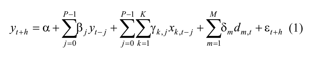
where

where
A General-to-Specific (GETS) Approach
In the GETS procedure, model selection is only applied to the elements of
Model Selection Using a Measure of Predictive Accuracy (MPA)
In this approach, model selection applies to all elements in
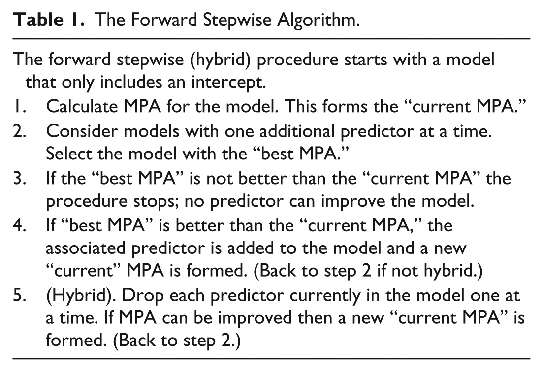
The forward stepwise regression starts with a model that includes only the intercept. Predictors are added one at a time, and the one that most improves the MPA is retained in the model. The procedure is repeated until no further improvement in the MPA can be achieved. In contrast to the forward procedure, the backward stepwise regression starts with a model that includes all predictors. Each predictor is removed from the model one at a time, and the one that mostly improves the MPA by being removed is eliminated. The procedure repeats until no further improvements in the MPA can be achieved. In the hybrid version of the forward (backward) stepwise regression, each time we add (drop) a predictor we also consider dropping (adding) a predictor. Obviously this is relevant in the forward (backward) procedure once at least three predictors have been added (dropped) to the model. Table 1 summarizes the forward stepwise (hybrid) procedure. All programming was implemented in R version 3.2.0 and is available on request. For more examples of stepwise selection process, see James et al. (2013).
The Forward Stepwise Algorithm.
The MPAs we consider are the usual information criteria, that is, the AIC defined as

the bias corrected AIC defined as

and BIC is defined as
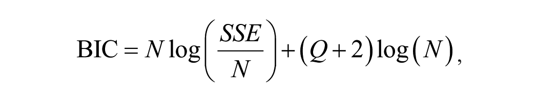
where SSE is the sum of squared errors, N is the number of observations used for estimation, and Q is the number of predictors in the model (excluding the intercept). The properties of the AIC and the BIC are well known. BIC will choose the same or fewer predictors compared with the AIC as it penalizes additional predictors more heavily than the AIC. Of the three, the one that has never been applied in the tourism literature is the AICc. The AICc is particularly useful in small samples with many predictors where the AIC is biased toward selecting too many predictors. The final MPA we consider is the cross-validation (CV) statistic by implementing leave-one-out cross-validation, which has also never been used in the tourism literature. When the number of observations is large, minimizing AIC is identical to minimizing the CV statistic (Stone 1977). Calculating the CV can be a time consuming process in other situations. Fortunately, for regression the CV statistic can be calculated very effectively by the following equation

where
Bagging Forecasts
Bagging or bootstrap aggregating was proposed by Leo Breiman in 1994 with the aim to improve unstable procedures from generating new learning sets. In our forecasting context, the aim of bagging is to reduce the variance of your forecast. The general idea simply put is the following. Using bootstrapping, which is a resampling technique, we generate additional samples for training our model(s) by drawing with replacement from the original data set. We refer to these as bootstrap samples. Let us assume we generate
The starting point is the predictive regression model in the form of equation (2). Forecasting with bagging involves generating a large number,

Generate a bootstrap sample

For each bootstrap sample, implement model selection and estimate the model from
The final forecast is then given by

In the empirical evaluation that follows, we find that instead of using the averaging across the
Data
Our case study aims to build predictive models to forecast Australian international tourism demand.
Dependent Variable
We consider quarterly tourist arrivals to Australia over the period 1981Q1 to 2012Q3 from six origin countries: Canada, Germany, Japan, New Zealand, United Kingdom, and the United States. The incoming tourist data are obtained from Tourism Research Australia: International Visitor Survey. Figure 1 provides time series plots of the arrivals data for each source country over the entire sample. The solid vertical line indicates 2008Q3 as the date of the Lehman Brother Bankruptcy (LBB), and the dashed line shows the beginning of the hold-out sample to be used for the forecast evaluation. The first four plots show a clear upward trend of tourist arrivals from Canada, United States, Germany, and United Kingdom. This increase seems to have been affected by the LBB and the global financial crisis that followed. Tourist arrivals from Japan are very different to all other source countries, showing a downward trend since the midnineties. Tourist arrivals from New Zealand also seem different from the other four countries, recovering quickly after the LBB and showing an upward trend quickly after that.
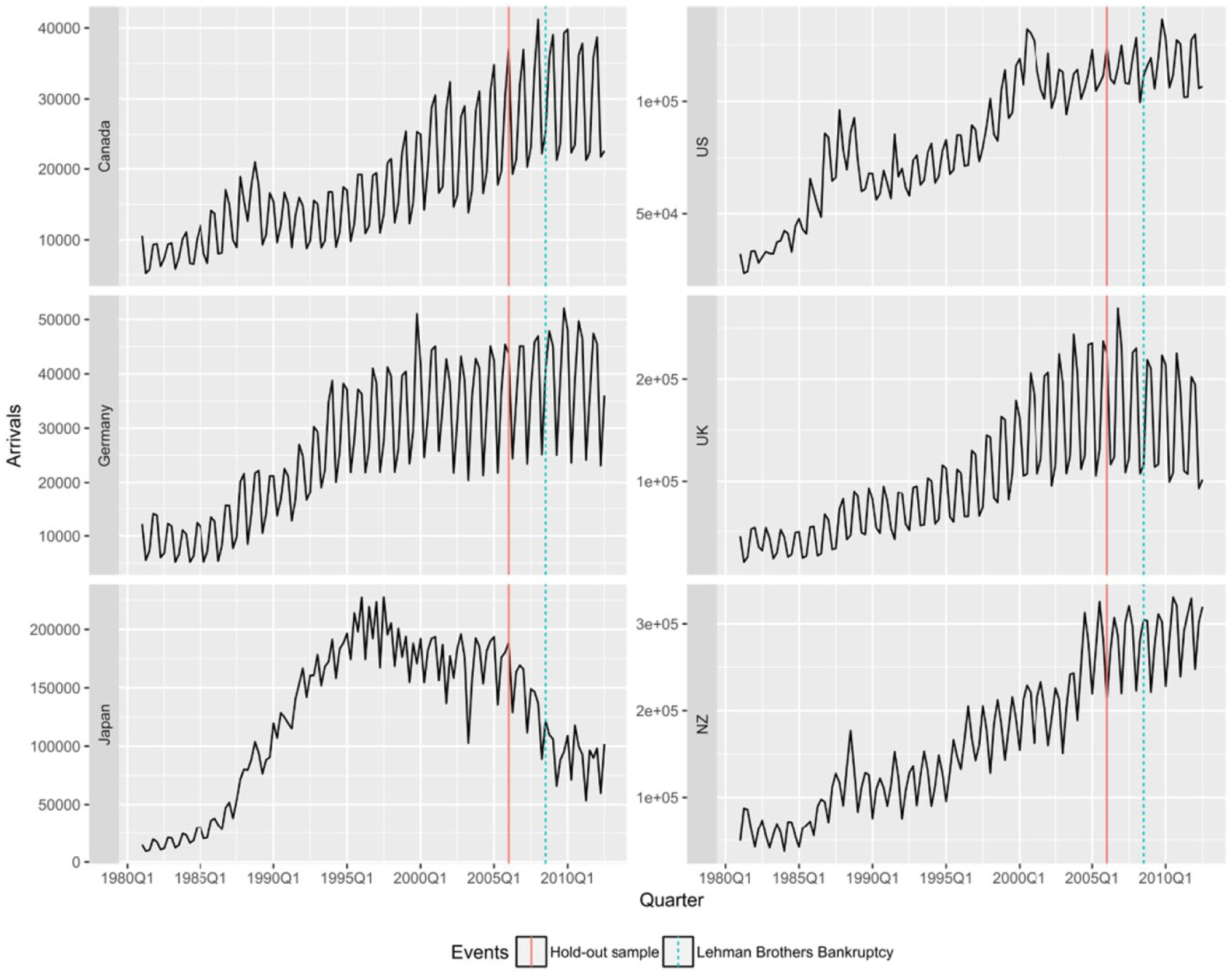
Tourist arrivals to Australia.
Figure 2 is a seasonal plot for the tourist arrivals time series, providing some visualization. Observing these, it becomes immediately obvious that seasonality between the first four source countries shows a consistent pattern, with the January (which is the summer period for Australia) and the October (including the beginning of summer and the Christmas and New Year’s holiday period) quarters being the peaks and the April and July quarters being the troughs. The one source country that is very different is New Zealand. Peak arrivals from New Zealand occur during the July quarter followed by the April and October quarters. Unlike all other source countries, the trough clearly occurs during the January (summer) quarter. The seasonal plots are also useful, revealing anomalies or one-off events. For example, in the U.S. plot, the peak arrivals for all July quarters occurred in 2000 during the Sydney Olympic games.
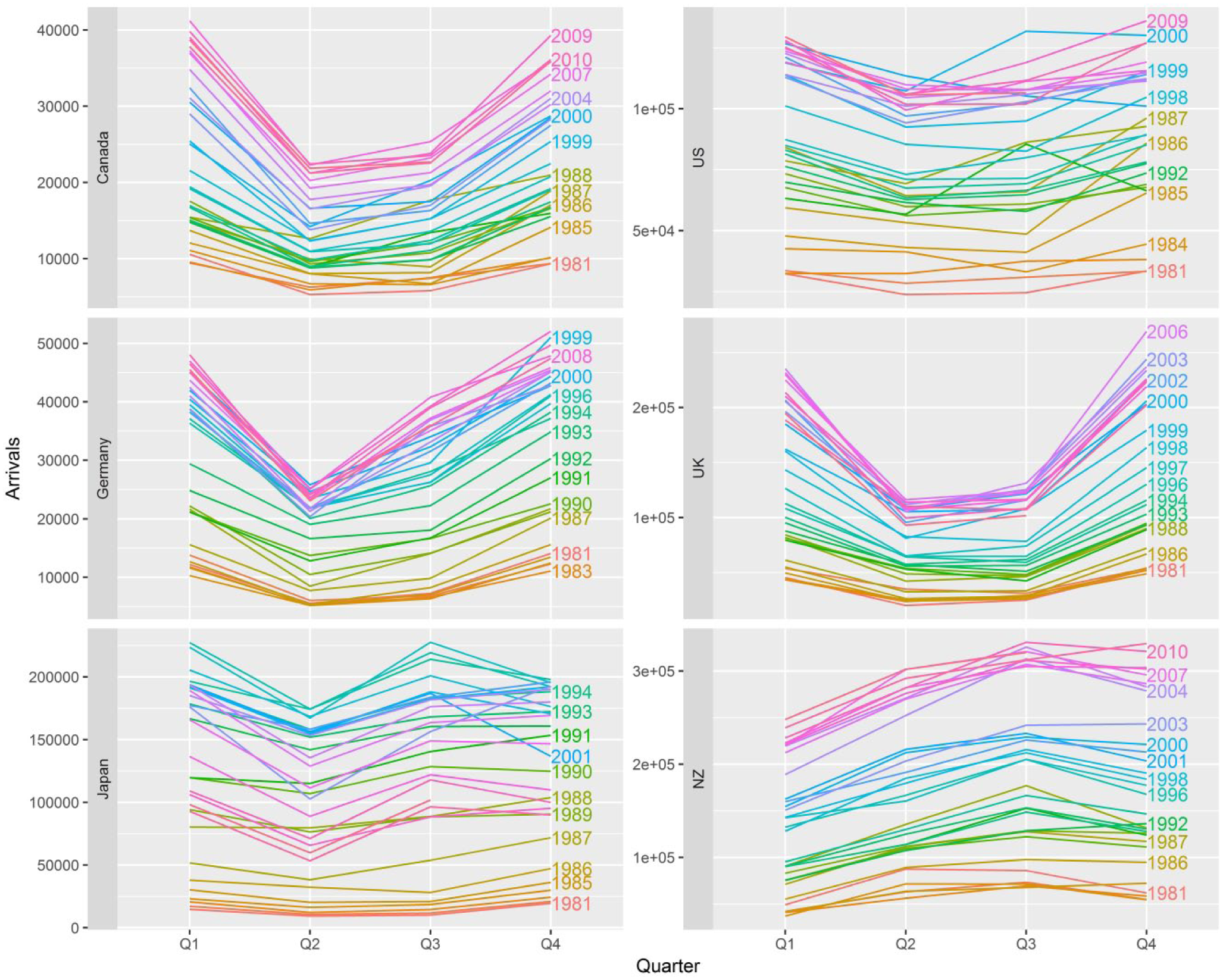
Seasonal plots of tourists arrivals to Australia.
Economic Predictors
Law of demand states that the demand for a good or service is inversely related to its price, ceteris paribus. This is measured by the own price variable defined as the ratio between CPIs and standardized by exchange rate

where

This predictor will obviously not be considered when New Zealand is the source country. Seasonally adjusted GDP in constant 2007 prices for the source countries using the expenditure approach and the unit currency of the source country is used as the income variable

The final economic variable considered is the interest rate spread defined as

where
Other Variables
Beside the four economic predictors, we also include seasonal dummies and two one-off dummy variables: one for the Sydney Olympics and one for the events of 9/11, which take the value of one for 2000Q3 and 2001Q3, respectively, and zero otherwise. Dummies for other one-off events such as the Bali bombings were not found to be selected.
Data Transformations
In the modeling procedures presented in the second section, both dependent variables and predictors need to be suitably transformed to stationary before entering the modeling framework. The time plots of the dependent variables clearly indicate a multiplicative and heteroscedastic seasonal pattern, and therefore all variables are first log transformed using natural logs. All dependent variables are deemed to require seasonal and first-order differencing with the exception of the U.S. arrivals, which only requires seasonal differencing. These decisions are reached following a sequence of seasonal (OCSB) and nonseasonal (ACF and KPSS) unit root tests and also after observing the ACF of the transformed series according to the tests. Table 2 summarizes the decisions after the hypothesis tests and the final transformations implemented on each of the dependant variables in order to achieve stationarity.
Variable Transformations to Achieve Stationarity.

Note: The first column indicates that each series was logged. An entry of 1(0) under the test columns indicates that a seasonal or nonseasonal unit root was (not) found. An entry of 1(0) under the differencing columns indicates the action taken after also observing the ACF of the differenced series. The final column indicates the final transformation implemented.
After considering both unit root tests (ADF and KPSS), the economic predictors are transformed as follows:
Forecast Evaluation Procedure
Forecast evaluation is implemented in an expanding window setup. The holdout sample begins in 2006Q1. Therefore, after transformations, there are

A competing model is estimated and forecast
Measures of Forecast Accuracy
Let


where
Benchmarks
The first benchmark we consider is an AR model that also includes the full set of dummy variables defined as

The dummy variables are always included in the AR model, and hence only lagged dependent variables will be selected. The maximum number of lags is 4, and the number of lags selected is determined by minimizing the AIC. As the predictive models using the GETS approach has the exact same lagged dependent variables as the AR model, any forecasting accuracy improvement over the AR model can be contributed to the predictors. This forms one of our natural benchmarks.
The other benchmark we use is the seasonal random walk model represented by a
Empirical Results
Table 3 summarizes the three classes of competing models in the forecast evaluations that follow. The first class of models are the predictive regressions build using statistical inference in the GETS algorithm. The second class of models are predictive regression models built by using MPAs, and the third class of models are our benchmarks. We apply bagging to both the first two classes of models in an effort to improve their forecast accuracy.
A Summary of the Competing Models.

Does Bagging Improve Accuracy in Forecasting Tourism Demand?
The first question we ask from our forecast results is whether implementing bagging on the predictive regression models improves their out-of-sample forecast accuracy. The evidence from this study is overwhelmingly affirmative. Table 4 shows the percentage change in forecast accuracy measures before and after bagging. A negative (positive) entry indicates a percentage decrease (increase) in the forecast accuracy measure. Hence for bagging to be effective negative entries are required in Table 4.
The Percentage Difference in Forecast Accuracy When Bagging Is Implemented to the Predictive Regression Models Compared to No Bagging.

Note: A negative (positive) entry indicates the percentage decrease (increase) in MAPE or RMSE when bagging is applied to each model. AIC = Akaike information criterion; AICc = bias-corrected AIC; BIC = Bayesian information criterion; GETS = general-to-specific; MAPE = mean absolute percentage error; MPA = measure of predictive accuracy; RMSE = root mean squared error.
In the majority of the cases across all six source countries, bagging has improved forecasting accuracy of GETS considering both MAPE and RMSE. The improvements are larger in size for MAPE than RMSE. On average across all the countries, bagging improved the forecasting performance of GETS for each forecast horizon. Furthermore, bagging is especially effective for 1- and 2-steps-ahead forecasts. For 1 and 2 steps ahead, bagging improved the MAPE of GETS forecasts for 22 of 24 cases (92%). For the RMSE, bagging improved forecast accuracy for 20 of 24 cases (83%). In general, there were more improvements for GETS 0.05 compared to GETS 0.01. This is to be expected as the GETS algorithm using a p value of 0.01 only chooses the most significant predictors and therefore will not allow bagging to generate diverse forecasts that we average over that provides the advantage of bagging.
In general, similar to the results for GETS, bagging also improves forecast accuracy for the predictive models selected by MPAs. Bagging improved forecast accuracy the least for BIC which is not surprising. As a consistent and the most parsimonious criterion with a heavy penalty component compared to other MPAs and similar to the GETS using a p value of 0.01, the reduction in forecast diversity impairs the improvements that can be achieved by bagging. Also similarly to the GETS results, bagging is most effective for 1- to 2-steps-ahead forecasts. For 1 step ahead for both MAPE and RMSE, all MPA models improved forecasting accuracy with the exception of the models for Canada.
Forecast Evaluations of Competing Models
The four panels in Figure 3 show the MAPE and RMSE respectively across all six countries.
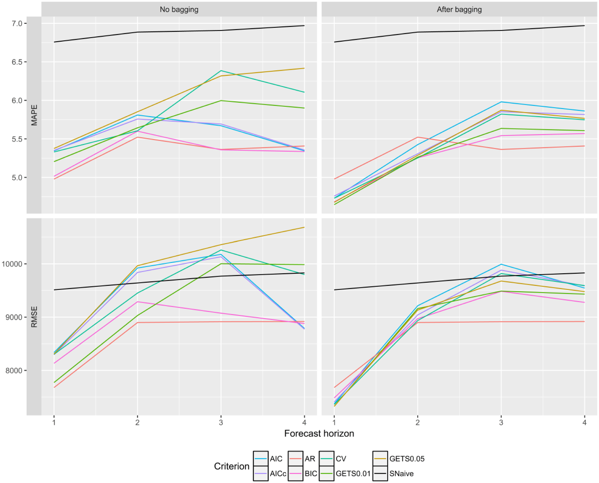
MAPE and RMSE for
These are complemented by the results presented in Table 5. A negative (positive) entry in Table 5 shows the percentage decrease (increase) in MAPE or RMSE over the SNaïve benchmark. A bold entry indicates that the predictive regression model is more accurate than the AR benchmark.
Percentage Difference in MAPE and RMSE between the Seasonal-Naïve Benchmark and the Predictive Regression Models.

Note: A negative (positive) entry indicates a decrease (increase) in the error measure compared with the seasonal-naïve benchmark. Bold entries indicate that the predictive regression model has performed better than the AR benchmark. AIC = Akaike information criterion; AICc = bias-corrected AIC; AR = Autoregressive benchmark; BIC = Bayesian information criterion; CV = leave-one-out cross-validation; GETS = general-to-specific; MAPE = mean absolute percentage error; MPA = measure of predictive accuracy; RMSE = root mean squared error.
One immediately obvious observation from Figure 3 is that all the dashed lines are squeezed downward when moving from the left-hand side (LHS) panels where no bagging is implemented to the right-hand side (RHS) panels where bagging is implemented. As expected, the variance of the forecasts across the models is damped. The band of the forecast error measure across the bagged alternatives is now much tighter than when bagging is not applied. All predictive regression models were more accurate than the SNaïve benchmark for all
Taking a closer look at the forecast results on a country-by-country basis, we identify two extreme cases. These are the cases of Japan and New Zealand. Tourist arrivals from Japan show a general downward strong trend since 1995. This makes the SNaïve forecasts inappropriate, and the predictive regression models perform much better than this benchmark for Japan. On the other hand, there is New Zealand where the SNaïve convincingly beats the predictive regression models. We should note that the individual country results are not presented here to save space but they are available on request. New Zealand is a special case for Australia. Although it is considered international travel, the economic and social ties between the two countries makes it arguably domestic in nature. This is initially identified by the seasonal plots shown in Figure 2. Furthermore, there have been discussions in the political arena since 2009 contemplating changing the actual status of the travel between the two countries to domestic (see, e.g., among others David Stone’s article in the New Zealand Herald; Stone 2009). Therefore, it may be the case that the economic variables used in the demand model may not be the best predictors for tourist arrivals from New Zealand as these variables may have a much smaller effect on domestic type travel. We should note that no matter what we did with New Zealand and for which period we looked at, the predictive regression models could not forecast any more accurately than the SNaïve benchmark. Given these results, we continue our analysis by removing these two countries from the results in order to remove the biases these two countries introduce.
Figure 4 and Table 6 show the MAPE and RMSE across the four countries (we have now removed Japan and New Zealand). We notice now that the SNaïve benchmark has become much more relevant and not easy to beat. For both MAPE and RMSE the predictive regression models forecast more accurately than the SNaïve benchmark only for
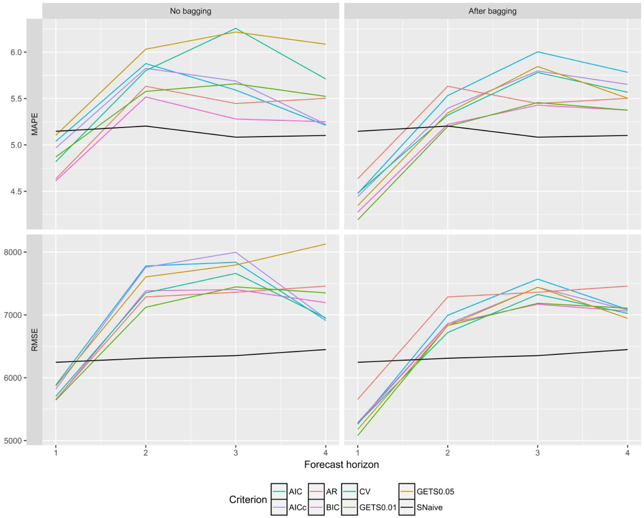
MAPE and RMSE for
Percentage Difference in MAPE and RMSE between the Seasonal Naïve Benchmark and the Predictive Regression Models Excluding NZ and Japan.

Note: a negative (positive) entry indicates a decrease (increase) in the error measure compared with the seasonal-naïve benchmark. Bold entries indicate that the predictive regression model has performed better than the AR benchmark. AIC = Akaike information criterion; AICc = bias-corrected AIC; AR = Autoregressive benchmark; BIC = Bayesian information criterion; CV = leave-one-out cross-validation; GETS = general-to-specific; MAPE = mean absolute percentage error; MPA = measure of predictive accuracy; NZ = New Zealand; RMSE = root mean squared error.
We next ask the question of why do the predictive regression models only forecast well for
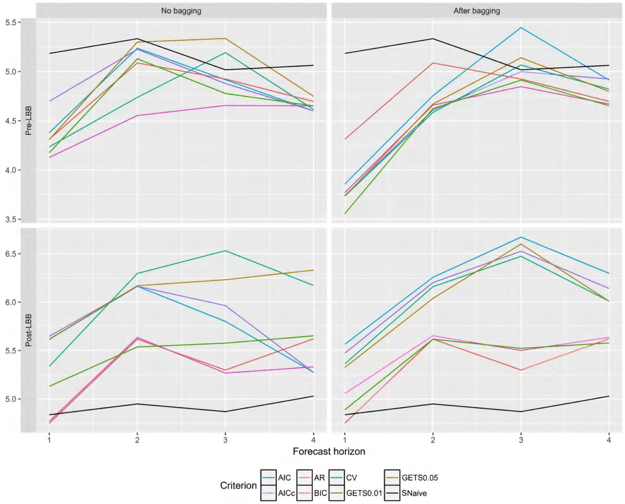
MAPE for
The results for the post-LBB period presented in Table 7 clearly show the failure of the predictive regression models to forecast any more accurately than either benchmark. This possibly highlights a breakdown in the predictive power invested in the economic predictors and their relationships with tourism demand. In this case, the results also clearly show that bagging does not in any way improve forecast accuracy. In fact it actually hinders it. For example the model selected by BIC performs closely and if anything better than the AR benchmark but only before bagging.
Percentage Difference in MAPE between the Seasonal Naïve Benchmark and the Predictive Regression Models for the Pre- and Post-LBB Periods Excluding NZ and Japan.

Note: A negative (positive) entry indicates a decrease (increase) in MAPE compared with the seasonal-naïve benchmark. Bold entries indicate that the predictive regression model has performed better than the AR benchmark. AIC = Akaike information criterion; AICc = bias-corrected AIC; AR = Autoregressive benchmark; BIC = Bayesian information criterion; CV = leave-one-out cross-validation; GETS = general-to-specific; MAPE = mean absolute percentage error; MPA = measure of predictive accuracy; NZ = New Zealand; RMSE = root mean squared error.
Concluding Remarks
In this study, we implement and examine fully automated model selection procedures in an effort to improve the out-of-sample forecast accuracy of causal econometric models commonly used in both academia and industry to forecast tourism demand. The first contribution of the article is to introduce to the tourism literature predictive regression models. These models have various advantages over models typically used. For example, unlike causal models, predictive regressions can be fully automated to generate forecasts. This is highly relevant to the tourism sector automated algorithms are required to generate forecasts such as the Hong Kong Tourism Demand Forecasting System. Obviously in contrast to pure time series approaches predictive regressions account for very important causal relationships. An alternative approach would be to treat all variables as endogenous in a multivariate VAR framework. However, dimensionality here is a challenge and techniques such as Bayesian estimation utilizing the so-called Minnesota prior need to be implemented, which arguably are very expensive and challenging to automate.
The second contribution of the paper is that we consider two broad variable selection procedures in order to achieve some parsimony and subsequently improved forecast accuracy for our models. In the first procedure known as the general-to-specific approach, predictors are selected using individual t statistics. In the second procedure, predictors are selected based on measures of predictive accuracy. The measures we consider are the AIC, the bias-corrected AICc, the BIC, and the cross-validation statistic. Using measures of predictive accuracy for model selection is a rarity in the tourism literature, which is concentrated on using statistical inference. Obviously, using t-tests is problematic in such a framework, where predictors are highly correlated. To our knowledge, this is the first time that the bias corrected AIC, which is important especially for small samples, and the cross-validation statistic are introduced to the literature. These criteria are now commonly used in applications of automated forecasting procedures (see, e.g., chapters 5, 7, and 8 in Hyndman and Athanasopoulos 2014). We encourage the application of these in forecasting tourism as well.
The third and arguably most important contribution of the paper is that we complement the implementation of variable selection procedures for predictive regressions with bootstrap aggregation, a procedure which aims to improve the predictive accuracy of the models based on resampling. We find overwhelming evidence that bagging improves the out-of-sample forecasting accuracy of the predictive regression models for predicting tourism demand, so much so that in many cases it is only after bagging that the predictive regressions become more accurate than simple benchmarks. We strongly recommend that such machine learning procedures (boosting is another alternative) should be adopted in the field of tourism and should be implemented in similar situations. Obviously, the disadvantage here is that there is a setup cost. However, automating these processes is straightforward and the gains are large. An interesting future research project would be to evaluate the contribution of such procedures beyond the one country considered here.
The final contribution of the article is the analysis of international tourist arrivals to Australia and the discovery of significant changes the global financial crisis triggered on the predictive power of typically used economic variables to predict tourism demand. The empirical results based on tourist arrivals data from six source markets suggested that the common economic factors used in the literature such as prices, exchange rates, and output are mostly reliable predictors for international tourism demand in Australia up to 2008Q3. Moreover, 2008Q3 marks the Lehman Brothers Bankruptcy (LBB), which triggered the beginning of the Global Financial Crisis (GFC). In general, the most accurate were the models built implementing the general-to-specific procedure with a p value 0.01 and the models built using BIC as the measure of predictive accuracy. These findings are in line with the principle of parsimony, which dictates that the simplest, more parsimonious models are often the best for forecasting. Similar conclusions for pure time series approaches have been drawn in the context of comprehensive forecasting competitions such as Makridakis and Hibon (2000). We should note here that these models were most accurate, and bagging was most effective for 1- and 2-steps-ahead forecasts during the pre-LBB period.
For the post-LBB period no predictive models were more accurate than the simple benchmarks; an AR model and a seasonal random walk. Furthermore, it was only for the post-LBB period that implementing bagging did not improve the forecast accuracy of the predictive regression models. It seems that the shock of the GFC may have significantly disturbed the economic relationships between tourism demand and the typically employed economic predictors. Obviously, this observation is based on Australian data and is limited within the general automated modeling framework employed here and therefore should be treated cautiously. There is scope in future studies to expand this automated framework to other countries. Furthermore, in an effort to improve forecast accuracy of predicate regressions per se there may be scope of relaxing somewhat the fully automated nature of the procedure and target source country–specific modeling challenges where effects of shocks such as the GFC can be modeled using more flexible functional forms such as nonlinear processes or linear models accounting for structural breaks.
Footnotes
Declaration of Conflicting Interests
The author(s) declared no potential conflicts of interest with respect to the research, authorship, and/or publication of this article.
Funding
The author(s) disclosed receipt of the following financial support for the research, authorship, and/or publication of this article: Song and Athanasopoulos acknowledge the financial support of the Hong Kong Research Grant Council (Grant No. PolyU 5969/13H). Athanasopoulos acknowledges the financial support of Australian Research Council Discovery Project DP 1413220.