




Abstract
This article develops a random utility model of tourist demand for agritourism destinations. Prior research has largely focused on modeling the effect of visitor characteristics and demographics on the demand for agritourism. In contrast, we analyze cross-section data on producer-reported visits to measure the effects of destination attributes. This allows us to examine whether tourists choose destinations based on landscape attributes. The destination choice model is applied to agritourism demand in Oklahoma. We calculate elasticities from both conditional logit and Poisson interpretations of the model. The results provide no evidence that landscapes affect the demand for single-day sites, but do suggest local land use plays a role in the demand for overnight destinations.
Introduction
Agritourism is an important and growing industry in the United States. Between 2007 and 2012, the number of farms providing agritourism and recreational services increased from 23,000 to 33,000, and aggregate receipts rose from $567 million to $704 million (USDA 2012). These figures do not include the thousands of other, nonfarm establishments that fall under the definition of agritourism, including farm heritage sites and rural businesses providing agricultural or outdoor-related recreation activities. Farm owners enter the tourism industry motivated primarily by the opportunity to supplement existing income sources (Nickerson, Black, and McCool 2001; McGehee and Kim 2004; Barbieri 2010; George et al. 2011; Lucha et al. 2016), although nonfinancial reasons are also important motivators (Blank 2002; George et al. 2011).
Researchers have responded to the growing demand for information about agritourism markets by studying the characteristics of producers and consumers. Existing studies of producers report on the motivations of farmers to enter the market (Getz and Carlsen 2000; Nickerson, Black, and McCool 2001; McGehee and Kim 2004; Ollenburg and Buckley 2007), product types (Phillip, Hunter, and Blackstock 2010; Ohe and Ciani 2011), production challenges (Che, Veeck, and Veeck 2005; Colton and Bissix 2005), and farmers’ personal satisfaction with the venture (Tew and Barbieri 2012; Chase, Kuehn, and Amsden 2013). Studies of agritourism consumers largely focus on demographics (Che, Veeck, and Veeck 2007; Nasers 2009; Ainley and Smale 2010; Brown and Hershey 2012). Until recently, little research investigated consumer preferences for agritourism destinations (Gao, Barbieri, and Valdivia 2013). However, there is growing recognition that consumer preferences are important in understanding the demand for agritourism (Santeramo and Barbieri 2016).
This article extends current research on farm and rural tourism by developing a demand model of agritourism destinations. By viewing these destinations as a differentiated products market, we are able to exploit variation in visitation levels, landscape features and on-site activities to learn about consumer preferences for destination attributes. 1 Individual, consumer-level data is often used to estimate similar demand models for outdoor recreation sites (e.g., see Moeltner and Von Haefen 2011; Paudel, Caffey, and Devkota 2011; Melstrom et al. 2015); however, our model is estimated using producer-reported data. Producer or aggregated data are the summaries of individual transactions with a company, which are often used to model the demand for differentiated consumer products in economic and marketing research (Berry 1994; Berry, Levinsohn, and Pakes 1995). By characterizing demand in this manner, we can analyze consumer preferences for destination attributes.
This article departs from the existing literature in two important ways. First, prior research on the demand for agritourism focuses on modeling the role of individual characteristics in participation and trip avidity (Rosenberger and Loomis 1999; Fleischer and Tsur 2000; Carpio, Wohlgenant, and Boonsaeng 2008; Hill et al. 2014). While personal characteristics capture important variation in individual tastes, insights from these models into preferences for landscape features are incomplete. One reason for this neglect is that preferences for differentiated products can be difficult to measure from revealed preference data, 2 for example because there may be little variation in the actual choices of visitors surveyed at one or a few destinations (Crouch et al. 2007). 3 To get around this problem, several articles in the agritourism literature use stated preference data derived from choice experiments to measure the effects of destination attributes on demand (Santeramo and Barbieri 2016). In contrast, we model the effect of actual destination attributes and landscapes on demand using visitation data from across a large number of agritourism destinations. To our knowledge, only Tchetchik, Fleischer, and Finkelshtain (2008) develop a similar model of agritourism destinations, although they focus on the effects of destination attributes at overnight stays while our data include single-day sites. 4 The effect of landscape attributes on demand is an important research question because scenic areas with public goods value could provide justification for policies to protect rural landscapes.
The second departure from previous work comes from estimating a utility theoretic model of tourism demand using producer-level data. Most studies of tourism demand use time series and econometric models to forecast demand, usually as a function of prices; see Crouch (1994), Song and Li (2008), and Song et al. (2012) for reviews. We model trips as a function of destination attributes using a random utility maximization (RUM) model; while RUM models have been used in microeconometric studies of tourism demand (e.g., see Lacher et al. 2013), ours is one of the first to estimate a RUM model using producer-reported data. The benefit of producer or aggregated data is that they can be collected from business records or market reports; thus, the data may be accessible to researchers without requiring costly surveys. A weakness of some travel demand models is omitting the effect of outside (nontourism) goods on demand (Crouch et al. 2007). However, we show that the RUM model can account for the role of outside goods by interpreting the elasticities in both a conditional logit and Poisson-based econometric framework, as has been done in studies of firm location choice (Schmidheiny and Brülhart 2011). Despite these innovations, analysts will find that our RUM-compatible demand function resembles existing single-equation models of tourism demand.
We apply our agritourism demand model to destinations in Oklahoma. The initial motivation for developing the model was to determine whether landscape attributes matter to visitors. In addition to presenting a model estimated on the full sample, we examine demand for single-day and overnight destinations independently. The results of this study suggest that landscape attributes have little effect on the demand for single-day visits, but play a more substantial role in the demand for overnight destinations.
Theoretical Framework and Estimation Strategy
We begin by specifying a RUM model of agritourism demand (see Haab and McConnell (2002) for an explication of RUM methodology). The utility of tourist

where

which is known as the conditional logit model.
RUM models are usually estimated with individual-level choice data (a tourist matched to a destination), but aggregated data (total trips to a destination) can also be used. If the analyst had individual-level choice data, she or he could estimate the model as a conditional logit (or a generalization thereof) and interpret the parameters as measuring consumer tastes for destination attributes. With aggregated data on tourism visits

where

If the attribute variables on the right-hand side were themselves logged, then equation (4) is analogous to the double-log arrivals model often used in tourism demand analysis (Song and Wong 2003; Song et al. 2010). However, one difference between our approach and those of earlier studies is that we use cross section data on destinations rather than time series to identify the role of predictive variables. Nevertheless, a sufficiently long time series or panel data could be used to parameterize a RUM model of tourism demand.
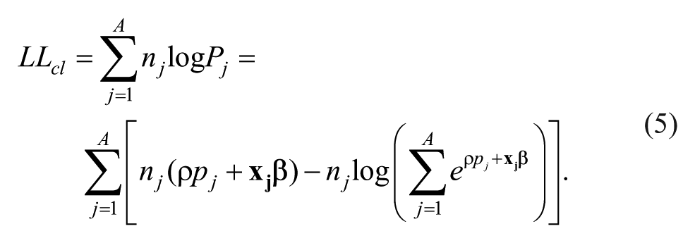
Whatever the source of variation, aggregated data can be used to estimate the parameters in equation (3) and thus measure consumer tastes for destination attributes exactly as described in equation (1). To see this, note that the conditional logit is estimated by maximizing the log-likelihood function
Now, the Poisson can be used to model the number of visits

The Poisson probability density function is

which yields the log-likelihood function

From the first-order condition with respect to
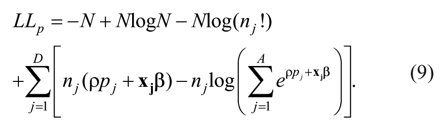
The first three terms are constant and the last term is identical to the right-hand side of equation (5). Thus, the conditional logit and Poisson are identical estimators (Guimarães, Figueirdo, and Woodward 2003). To estimate the RUM model with aggregated data, Poisson regression can be applied to equation (3), which in our application models the number of visits to a cross section of agritourism destinations. 6
Although the RUM model of agritourism demand can be estimated equivalently as a conditional logit or a Poisson, the two econometric models differ in terms of their implied elasticities. This is because the conditional logit assumes the number of tourist visits is fixed and that changes in destination attributes affect only the distribution of visits across destinations. Thus, it assumes an increase in visits to one destination are offset by a decrease in visits to the other destinations. In contrast, the Poisson assumes there is no cross-site substitution, so changes in the attributes of one destination do not affect the number of visits elsewhere, and an additional visit at one site will raise the total number of visits in the market by one. Schmidheiny and Brülhart (2011) show the conditional logit and Poisson models can therefore be viewed as polar cases, and that the elasticities implied by the two models are boundary values on the true effect.
With the price variable in levels (rather than in logs), the elasticity of an own-price change at destination j implied by the conditional logit is

Equation (10) measures the percentage change in expected visits to j for a one unit change in price. If price was in logs, then the elasticity would be

Equation (11) measures the percentage change in expected visits to

while the cross-price elasticity is

Equations (10) and (12) show that the Poisson predicts more elastic responses from changes in a destination’s own-price, while equations (11) and (13) show that the conditional logit predicts a more elastic response from changes in the prices of other destinations. In fact, because the basic RUM model excludes tourists who did not visit any of the destinations in the study, the true elasticity lies between the predictions made by the two models. Schmidheiny and Brülhart (2011) show that when the choice model is generalized to account for non-participation or other purchases (e.g., as in Crouch et al. (2007)), then the elasticities implied by the two models act as bounds on the actual elasticity. We illustrate the changes implied by both models for several variables later in the results.
With producer-reported data we prefer to use the Poisson (as the estimator) to parameterize the RUM model but, as we have shown, the conditional logit would estimate identical coefficients. We expect analysts working with similar data will find it easier to estimate RUM models using the Poisson, as it simply involves regressing the number of visits on the destination characteristics, and thus avoids the transformations that may be required by statistical software to implement the conditional logit. Otherwise, for applications like ours the only difference between these two models lies in how they predict shifts in demand using the parameter estimates.
Data
Data on agritourism producers were gathered by the authors through a mail survey. The Oklahoma Department of Agriculture, Food and Forestry (ODAFF) provided a list of state-registered agritourism producers. This list included 355 destinations, but for the purposes of the survey, which focused on producers, 64 farmers markets in the list were removed. The remaining 291 producers were invited to participate in the survey in January 2015 following the protocols outlined by Dillman, Smyth, and Christian (2014). The initial mailing included a booklet questionnaire and an individualized, hand-signed letter describing the purpose of the survey. The cover page of the booklet was designed to coordinate with the writing, images, and symbols used by the ODAFF agritourism marketing program. The rest of the questionnaire was split into 5 sections that included questions about the business’s characteristics, customers, challenges, future plans, and owner demographics. For the purposes of this study, the booklet included the question “How many visitors did your Agritourism business receive in 2014?” The week following the mailing of the questionnaire, a postcard was sent out to the entire sample to remind participants to complete and return their questionnaire. Two weeks later, a second questionnaire was mailed to nonrespondents. Participants who had undeliverable surveys because of a wrong address in the first mailing were researched via the Internet for a new address, to which the second questionnaire was sent. A final reminder postcard was mailed out to nonrespondents one week following the second questionnaire. The overall response rate was 65%, and after removing undeliverable addresses, the response rate was 67%. In this study, 35 observations could not be used because the number of visitors was not reported by the producer. This left 155 usable questionnaires, which is an adjusted response rate of 54%.
Modeled destination attributes include land cover, owner demographics, and indicators for the product offered at the destination. Land cover includes cropland, forest, scrubland, developed land, and surface water area in square miles in the destination county. These data were collected from published U.S. Forest Service reports. 7 To avoid perfect multicollinearity, scrubland area was omitted and used as the reference land cover category. All land cover variables were put into the model in logs. Demographics include age (measured in logs), a dummy variable for college degree, and a dummy variable for American Indians. 8 The typical owner is in his or her late 50s, holds a college degree, and is not an American Indian (Table 1). We sort single-day and overnight destinations into 11 types (as developed by ODAFF), which range from exotic animals to u-picks to wineries. We include dummy variables for each type, using wineries as the excluded category.
Summary Statistics of the Variables Used in the Agritourism Demand Models.

We used two variables as proxies for the price of visiting a destination. First, distance to the nearest metropolitan area was used as a proxy for day visitors’ driving distance to single-day destinations, which is likely the largest component of the exogenous cost (in terms of time and money) of a visit. 9 To construct this measure, we used PC*miler software to calculate the driving distance in miles to the city centers of Oklahoma City, Tulsa, and Dallas, TX. We then selected the shortest distance among the three for each single-day destination as a measure of the proximity of the site to consumers. However, we fixed the effect of the distance variable to zero for visits to overnight destinations, so the effect of distance (to nearest metropolitan area) in the model is measured only for single-day sites. Second, the minimum per night room cost was used as a proxy for the price of staying at an overnight destination. 10 The effect of this price was fixed at zero for visits to single-day destinations.
To test for preference heterogeneity between day and overnight visitors, we divided the sample into destinations catering primarily on overnight farm and ranch guests and destinations focused on day visitors. That is, after using the full sample, we re-estimate the model using the single-day sites and again using the overnight destinations; these subsamples contain 121 and 34 observations divided among nine and two product types, respectively. We can test the hypothesis of preference heterogeneity between overnight and day visitors by comparing the model estimated on the full sample to the models estimated on the two subsamples.
Results
This section applies the RUM model of agritourism demand to the Oklahoma producer data. Three demand models were estimated: (1) A model of visits to all destinations, (2) a model of visits to single-day destinations, and (3) a model of visits to overnight destinations. The regressors are the same in the two models, except for the distance, price, and product dummy variables.
A common concern in econometric modeling is model misspecification. When relevant variables are unobserved or distributional assumptions fail, standard errors are often biased toward zero and thus overstate the precision of the estimated parameters. Several authors have examined this issue in conditional logit models of recreation demand that are similar in form to our own agritourism demand model (Murdock 2006; Melstrom and Jayasekera 2017). The same problem applies here, whether the Poisson or the conditional logit estimator is used to estimate the RUM coefficients (the standard errors, like the parameters, are identical in both cases). This bias is commonly interpreted in Poisson models as either overdispersion or underdispersion, due to violations of variance-mean equality (equidispersion). Following Hilbe (2011), we conducted a likelihood ratio test for variance-mean equality in the two models. The test failed at the 0.05 level in all models. We therefore report Huber-White errors, which provide robust inference under model misspecification.
The estimates from the full sample provide strong evidence of systematic differences in visits across product types, but little evidence that landscape attributes matter (Table 2). Overnight and hunting destinations tend to get the fewest visitors, while sites that focus on farm heritage, mazes, and pumpkin patches attract the most visitors. Visitation to exotic animal sites, specialty crops, trailriding, u-picks, and wineries lie between these two extremes. None of the land cover variables are significant at the 0.05 level, although the effect of forest is positive and significant at the 0.10 level, which suggests that agritourists in Oklahoma may favor destinations in forested landscapes. 11 The estimates also indicate that destinations owned by college graduates draw in more visitors than those owned by non–college graduates.
Results of the Agritourism Demand Models.
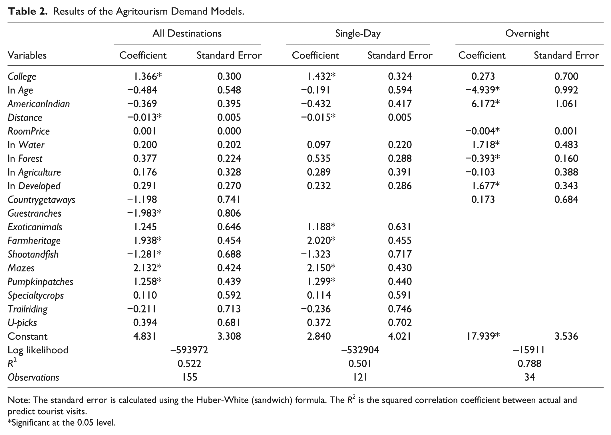
Note: The standard error is calculated using the Huber-White (sandwich) formula. The R2 is the squared correlation coefficient between actual and predict tourist visits.
Significant at the 0.05 level.
The estimates from the full sample mask important differences between the single-day and overnight destinations. We find that estimating separate models generates a significantly better fit to the data. Using a likelihood ratio test, we easily reject the hypothesis that the regressors have the same effects at single-day and overnight destinations.
12
Nevertheless, all three models fit the data reasonably well, with
Few destination attributes are significant in the single-day destination model except for the product dummies. Only the effect of distance is significant, which, being negative, implies that single-day destinations receive fewer visitors the farther they are from a metropolitan area. The coefficients on distance and the other variables measured in levels can be converted into approximate percentage changes using the formula
Relative to single-day sites, the results imply that land use matters in the choice of an overnight destination. The variables for water, forest, agricultural, and developed land area together explain about 40% of the variation in overnight visits. Relative to the omitted category, the effects of water, forest, and developed land are statistically significant at the 0.05 level. The coefficient on agriculture is negative but not individually significant. However, an F test of all four land cover variables finds the group to be highly statistically significant
Discussion
Landscape attributes appear to play a more significant role in agritourism consumer preferences for overnight destinations than single-day sites. None of the effects of land cover are significantly different from each other at acceptable confidence levels in the single-day destination model, suggesting that day visitors do not attach much importance to landscape attributes. On the other hand, holding all else equal, more visitation is associated with overnight destinations in counties with relatively large areas of water and developed land. 13 This could be because overnight trips tend to be multipurpose, and tourists prefer to stay near water-based recreation opportunities and urban areas with access to restaurants, shopping, and cultural amenities. There may also be a concentration of tourist activities in developed areas, which creates agglomeration benefits for visitors. Demand for agritourism destinations also appears to be influenced by access costs: Systematic differences in visitation are associated with proximity to metropolitan areas at single-day sites and room prices at overnight destinations.
The coefficients in Table 2 can be used to compute the own and cross-attribute elasticities implied by the conditional logit and the Poisson. We calculated these changes for the price and water variables using equations (10)–(13) (Table 3). The Poisson cross-elasticity is zero by assumption, as is the change in total visits predicted by the conditional logit. The differences between the conditional logit and Poisson-implied elasticities are practically indistinguishable when the model is applied to single-day sites: −1.12 for the conditional logit versus −1.13 for the Poisson for a one-mile increase in distance, and 0.96 for the conditional logit versus 0.97 for the Poisson for a 1% increase in water area. But the elasticities diverge modestly when calculated for overnight destinations: −0.74 for the conditional logit versus −0.78 for the Poisson for a one-dollar increase in price, and 1.67 for the conditional logit versus 1.72 for the Poisson for a 1% increase in water area. The size of these differences is an empirical issue and increase in cases where the parameter is larger and there are fewer substitutes (destinations). Differences become more apparent when changes are computed in terms of total visits.
Average Estimated Elasticities from the Demand Models.

For managers concerned about tourist demand, the implied elasticities can be used to guide decision making. The price elasticity implies that on average, accommodation prices are relatively inelastic; thus, owners/managers of overnight destinations could increase revenues by increasing prices on the margin. Our results also show that locating a day site in a county with large surface water resources is generally preferable over other attributes, except proximity to a metropolitan area. However, this comparison should be made with caution, because the effect of water was not estimated with precision in the single-day destinations model. For overnight destinations, there is little difference attributable to more local development than to more water, although if given the choice between a primarily agricultural county and a relatively more developed county, one should expect visitation to be higher for the latter, holding other attributes constant. Our results also imply that overnight destinations should not expect much of a difference in tourism demand, whether the business is marketed as a country getaway or a guest ranch, although single-day sites can expected significant differences in demand based on products, with more tourists visiting businesses with fall activities (such as mazes and pumpkin patches) and farm heritage than other types of sites.
Agritourism marketing in Oklahoma focuses on encouraging residents to drive out and visit farm and rural businesses. Our results shows it matters to consumers where these destinations are located. Single-day destinations near metropolitan areas tend to attract more visitors compared with destinations farther away, probably because consumers prefer to visits day sites close to home. Overnight destinations located in highly rural areas attract the fewest visitors. Marketing campaigns could focus on promoting the single-day sites in the communities around those sites to encourage tourism. Our results also suggest overnight destinations could benefit from marketing that convinces consumers that the area around the destination combines other reasons for travel, particularly in developed areas.
Although our estimates imply that local land use can affect the demand for overnight agritourism destinations, they do not provide justification for preserving rural, agricultural landscapes as public goods. This conclusion confirms the results of several earlier agritourism studies: Tchetchik, Fleischer, and Finkelshtain (2008) estimated a RUM model of Israeli agritourism demand from revealed preference data and found that tourists preferred overnight destinations located in communities with infrastructure and amenities, just as we found tourists in Oklahoma preferred overnight destinations in developed counties. However, Tchetchik, Fleischer, and Finkelshtain (2008) did not find evidence that agricultural ambiance was directly valued by tourists. Rosenberger and Loomis (1999) used a combined revealed-and-stated preference research design to study the effects of land use on tourist visits to a Rocky Mountain resort town. They concluded that conversion of agricultural land to urban and tourism development would not result in a loss in benefits to tourists. Similarly, in our demand model, tourist visits did not relate significantly to agricultural land area.
There are several caveats to this analysis that we should draw attention to. Local landscapes were described by county-level land cover. While research in the recreation demand literature often describes physical destination attributes at the county level, agritourism consumers may be more concerned about the landscape adjacent to the site. If land cover poorly proxies for the landscape ambiance around a farm destination, then measurement error could be obscuring the importance of landscapes in tourists’ destination choice. Visitor taste heterogeneity was incorporated into the model by separating the sample into overnight destinations and day sites, but visitors to the latter may not view all sites as good substitutes, requiring further division of the market. Another limitation of our study is the size of the agritourism market in Oklahoma. This left only 34 observations to estimate the demand model for overnight destinations, so some caution is warranted in interpreting the parameters (although we found part of our results were consistent with prior research). Finally, our data set was not rich enough to control for tourist characteristics or unobserved site attributes, which can play an important role in aggregate tourism demand (Carpio, Wohlgenant, and Boonsaeng 2008; Tchetchik, Fleischer, and Finkelshtain 2008). 14 By incorporating individual-level data and/or addressing unobserved site attributes, future work may be able to obtain more precise parameter estimates.
Conclusion
We analyzed the demand for agritourism in Oklahoma. Our results provide no evidence that day visitors prefer destinations in agricultural or developed landscapes, with most of the variation in visits explained by the type of product offered at the site and the distance to the nearest major metropolitan area. Farm heritage sites, mazes and pumpkin patches are the most popular products in this market. Landscape characteristics play a more important role in the demand for overnight agritourism destinations. Access to water resources and urban conveniences are associated with more tourist visits in this case.
We developed a random utility model to analyze the demand for agritourism destinations. We used producer-level rather than individual-level (tourist-level) data to parameterize the model. The procedure used in this article regresses the number of visits to each site on the attributes of these sites. This is akin to the procedure that some analysts use to model the demand for differentiated consumer products with aggregated data on market shares and product attributes. It is also similar to the approach in tourism demand research that estimates the effect of destination attributes and origin-country characteristics on travel in single-equation models. The procedure described in this article is easy to implement and is utility-theoretic. It does not require individual visitor data, only information on in-bound travel to each destination, although visitor-level data would allow the analyst to model individual taste heterogeneity.
Footnotes
Acknowledgements
The authors thank Jamie Cummings for her assistance in working with agritourism producers.
Declaration of Conflicting Interests
The author(s) declared no potential conflicts of interest with respect to the research, authorship, and/or publication of this article.
Funding
The author(s) disclosed receipt of the following financial support for the research, authorship, and/or publication of this article: This work was supported by the USDA National Institute of Food and Agriculture and the Division of Agricultural Sciences and Natural Resources at Oklahoma State University.