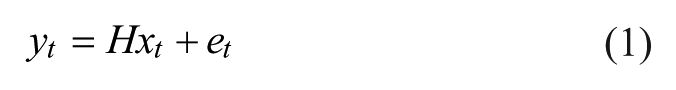
Forecasting Seasonal Tourism Demand Using a Multiseries Structural Time Series Method

Abstract

Multivariate forecasting methods are intuitively appealing since they are able to capture the interseries dependencies, and therefore may forecast more accurately. This study proposes a multiseries structural time series method based on a novel data restacking technique as an alternative approach to seasonal tourism demand forecasting. The proposed approach is analogous to the multivariate method but only requires one variable. In this study, a quarterly tourism demand series is split into four component series, each component representing the demand in a particular quarter of each year; the component series are then restacked to build a multiseries structural time series model. Empirical evidence from Hong Kong inbound tourism demand forecasting shows that the newly proposed approach improves the forecast accuracy, compared with traditional univariate models.

Keywords

multivariate structural time series model seasonality tourism demand forecasting

Introduction

Tourist flows in most destinations feature seasonal variations. Seasonality is one of the most important and distinctive characteristics of tourism demand and has important impacts on the planning and operation of tourism businesses and destination management with respect to infrastructure and resource allocation. Tourism demand typically displays seasonal patterns. There are a number of pros and cons from the perspectives of the local community, businesses, and the government. For a tourism destination, seasonality often results in overuse of infrastructure and facilities during peak seasons, which may further lead to the reduction of local residents’ quality of life and even social conflicts between tourists and the local community (Butler 2001). When the peak season is short, businesses need to cover the fixed costs throughout the year with profits generated in a limited time. Furthermore, seasonality in tourism demand may have a destabilizing effect on other economic sectors of a destination country or region given their economic linkages and competition on resources such as capital and labor (Lim and McAleer 2001). Despite the overwhelming impression of various challenges caused by seasonality in tourism demand, its positive impact on a destination’s residents and community should be acknowledged as well. Butler (2001) argues that for some destinations, the low season is the only time when the local population can engage in some social and cultural activities in a “normal” manner. The off-peak season would allow resources to be regenerated. Infrastructure and maintenance works can also be undertaken with very low impact.

Nevertheless, changing seasonality has been viewed as a challenge by tourism businesses. In regions with changing seasonal patterns, seasonal tourism income is difficult to predict. This consequently poses difficulties in getting access to investment that leads to high risk of operations (Butler 2001; Hinch and Jackson 2000). Changing seasonality may also cause challenges in employing sufficient qualified staff during an unpredicted peak season, which can lead to the reduction of service quality and tourist satisfaction (Pegg, Patterson, and Gariddo 2012).

Hence, seasonality has significant implications for both tourism-related policy making and business planning, and such implications are not only related to the tourism industry but also the rest of an economy. As such, seasonality in tourism has been recognized as an important concern of tourism research and one that deserves closer investigation (Rodrigues and Gouveia 2004). In particular, research on seasonal tourism demand forecasting plays an important role in assisting evidence-based decision making by tourism organizations and governments. Accurate forecasts of seasonal tourist flows can help decision makers to enhance the efficiency of their strategic planning and reduce the risk of decision failures. Therefore, both scholars and practitioners have been exploring methods to improve the accuracy of seasonal tourism demand forecasting. The present study seeks to add to this ongoing endeavor. Different from most of the previous studies in this field, this study provides an alternative approach that does not require modeling seasonal patterns explicitly.

Seasonality and Tourism Demand Forecasting

Modeling seasonal variations in a tourism time series has become an important issue in tourism forecasting in recent years (Kulendran and Wong 2005). To understand the nature of seasonality in tourism demand and capture it appropriately, we need to start with the definition of seasonality. From an economic perspective, Hylleberg (1992, 4) defines seasonality as follows:

Seasonality is the systematic, although not necessarily regular, intra-year movement caused by changes of the weather, the calendar, and timing of decisions, directly or indirectly through the production and consumption decisions made by the agents of the economy. These decisions are influenced by the endowments, the expectations and the preferences of the agents, and the production techniques available in the economy.

An important implication in this definition is that the seasonality can be driven by a wide range of factors, which could result in different seasonal patterns. When the fluctuations in timing and magnitude follow a mathematical/statistical pattern, the seasonal variation may be deterministic. On the other hand, if the seasonal pattern tends to change over time, or when the timing is regular but the magnitude is not, the seasonality should be treated as stochastic.

It has always been a challenging question whether the seasonal fluctuations are best viewed as deterministic or not. Kim and Moosa (2001, 382) note that “no conclusive evidence was found as to whether one should treat seasonality as stochastic or deterministic.” Some empirical evidence in both the general economic literature (e.g., Osborn, Harevi, and Birchenhall 1999) and the tourism literature (e.g., Kim 1999) suggests that the deterministic seasonality may be appropriate in modeling and forecasting the seasonal time series, while the assumption of stochastic seasonality has been more popular in recent studies (e.g., Lim and McAleer 2001). The following sections will review some commonly used methods in dealing with deterministic and stochastic seasonality of a tourism time series.

Deterministic Seasonality

Traditional methods of seasonal tourism forecasting generally regard seasonality as deterministic. This concept describes a process with a seasonal unconditional mean that varies with the season of the year. Therefore, deterministic seasonality can be expressed by a seasonal dummy variable representation. Based on the concept of deterministic seasonality, extensive research has been done to separate the seasonal component from a time series to generate a seasonally adjusted series (e.g., the X-11 method and its variants). In a tourism context, Lim and McAleer (2001) apply a moving average technique to separate the seasonal component from some monthly tourist arrivals series, and calculate monthly indices to show different degrees of tourist fluctuations across 12 months. However, as the authors acknowledge, such attempts may not be effective for forecasting, because such adjustments may remove not only seasonal fluctuations but also some of the trend and cyclical variations in the tourism series, given their correlations between each other. In addition, seasonally adjusted or deseasonalized series are only useful in predicting long-term trends.

Stochastic Seasonality

There are generally two types of stochastic seasonality in time series, namely, stochastic stationary and stochastic nonstationary processes. Stochastic stationary seasonality implies that the seasonal pattern tends to change over time, but the magnitude of the seasonal variation does not tend to change over time. With stochastic nonstationary seasonality, the seasonal pattern changes over time, and the typical magnitude of the variation also tends to increase year after year. It should be noted that some stochastic processes have a deterministic process as a “special case.” As pointed out by Miron (1994), whether a series should be modeled as a deterministic seasonal process or as a seasonal unit root process should be determined by seasonal unit roots. However, for finite sample sizes, it may be difficult to discriminate between deterministic seasonality and a seasonal unit root process, as they exhibit similar empirical properties (Ghysels and Osborn 2001). Nonetheless, recent empirical evidence suggests that stochastic seasonality is more appropriate for tourism demand modeling and forecasting (e.g., Lim and McAleer 2001; Song et al. 2011).

Broadly, there are two commonly used methods to model stochastic seasonality in tourism demand. The first one is the Box-Jenkins Approach, where stochastic seasonality is usually analyzed by the seasonal autoregressive integrated moving average (SARIMA) family of seasonal unit root models. The general Box-Jenkins model allows for seasonality with seasonal differences, seasonal autoregressive terms, and seasonal moving average terms. As most seasonal time series exhibit an increasing trend and/or seasonal variations, both seasonal and nonseasonal differencing are often used to stabilize the time series. The SARIMA models are most widely used in seasonal tourism demand forecasting and perform reasonably well (e.g., Alleyne 2006; Cho 2001; Goh and Law 2002; Kulendran and King 1997; Kulendran and Witt 2003b; Kulendran and Wong 2005; Oh and Morzuch 2005).

The second approach to handling stochastic seasonality in tourism demand is based on the unobserved component approach, often in state space form. The most popular model in this family is the structural time series model (STSM), which normally decomposes a time series into its trend, seasonal, and irregular components and regards these components as stochastic.

The originally proposed STSM assumes that the disturbances of the measurement and transition equations are mutually independent, which implies a multiple source of error (MSOE) for these equations. Anderson and Moore (1979) and Snyder (1985) outline an innovations form of state space models with a single source of error (SSOE) that drives all measurement and transition equations. The SSOE scheme is an important alternative as it offers advantages over the MSOE formulation in terms of both theoretical properties and empirical application. Because of the above independence assumption of MSOE, the variance matrix of the transition equation is constrained as a symmetric positive deﬁnite matrix. The corresponding parameter space of MSOE models is therefore smaller compared to that of the SSOE counterpart (Leeds 2000). Among other useful theoretical properties, the SSOE scheme is the only formulation in which the estimates of state variables converge to their true values (Ord et al. 2005). Empirically, it has been found that the SSOE models generally produce more accurate forecasts over the MSOE specifications when the true parameters lie outside the MSOE parameter space (Leeds 2000).

With an SSOE formulation, innovations state space models for exponential smoothing (often labeled as ETS) have also been introduced to tourism forecasting recently (e.g., Athanasopoulos et al. 2011). In terms of the treatment of seasonality, the innovations scheme is similar to the standard STSM in that a seasonal component is explicitly modeled in a stochastic way. In a tourism forecasting competition exercise, Athanasopoulos et al. (2011) show that the ETS performs particularly well once monthly data are used, but less so with quarterly data in use.

The STSM has been applied to tourism demand forecasting over the past two decades, although the number of applications is still limited. Examples include González and Moral (1995, 1996), Kulendran and King (1997), Kulendran and Witt (2003a), Song et al. (2011), and Turner and Witt (2001). The STSM’s forecasting performance in these studies has been consistently good. For example, Kon and Turner (2005) show that STSM outperforms all its competitors, including naïve, artificial neural network and exponential smoothing models. Between the SARIMA model and STSM, Kulendran and Witt (2003a) and Song et al. (2011) both present empirical evidence of STSM’s superiority.

In addition to the above methods, other techniques such as artificial intelligence methods have been applied to modeling and forecasting seasonal tourism demand. Given the space constraints and no direct relevance to the present study, they are omitted here. Explanations of other tourism forecasting methods and their applications are provided by Goh and Law (2012) and Li, Song, and Witt (2005) in their comprehensive reviews of a broad range of tourism forecasting methods. Among all of the seasonal tourism demand forecasting studies, seasonality is always dealt with in an “explicit” manner. In other words, a decision has to be made regarding whether seasonality should be modeled in a deterministic or stochastic way, or whether a seasonal adjustment should be exercised with an attempt to remove seasonal variations from the time series concerned.

As discussed above, these approaches all have their limitations. Although stochastic seasonality has been applied more often in recent studies, a general mix of various causes of seasonal fluctuations in any tourism demand series leads to no conclusive evidence on how seasonality should be treated (Kim and Moosa 2001). As such, choosing either way to model seasonality may not be ideal, which will potentially affect the forecast accuracy of the model.

Another observation from previous tourism demand forecasting literature is that most existing tourism studies are based on a univariate and single-equation setting; in other words, each model is specified to fit only one tourism demand series. To forecast m tourist flows (such as visitor arrivals from one country of origin to m destinations), m time series models would be specified, estimated, and forecast separately. In such an isolated way to generate tourism forecasts, the potential association among individual flows has been totally ignored. Capturing the long-term dynamic interrelationship between time series may result in more accurate forecasts (Athanasopoulos and de Silva 2012). This thought leads to further exploration of multivariate time series forecasting.

Multivariate Time Series Forecasting Models

As suggested above, a key advantage of the multivariate approach is that interrelationships between series can be gauged. The importance of this feature has been acknowledged by a number of scholars. For example, de Silva, Hyndman, and Snyder (2009, 1070) argue that “this feature cannot be underestimated as it is naïve to consider an economic variable in isolation.” There are various multivariate forecasting methods, such as econometric simultaneous equation and noncausal multiple time series (or vector) models. This study only focuses on the causal multivariate time series models.

Compared to the development of univariate forecasting models, there has been relatively little work in developing multivariate forecasting methods, despite being advocated by multiple scholars such as Chatfield (1988), Ord (1988), and De Gooijer and Hyndman (2006). The first multivariate approach, a vector ARMA model, is initially derived and discussed by Quenouille (1957); the first multivariate structural time series specification is proposed by Jones (1966). Further developments of multivariate techniques are associated with the development of computer software to implement such models. Key contributors to this development include Harvey (1989) and Durbin and Koopman (2012). They extend the STSM from a univariate formulation to a multivariate setting under the MSOE scheme. Taking the SSOE approach, de Silva, Hyndman, and Snyder (2010) extend the class of univariate innovations state space models to a vector innovations structural time series (VISTS) framework.

The motivation of the above exploration of multivariate time series models is to “exploit potential inter-series dependency to improve forecasting performance” (Chatfield 1988, 416). Many empirical studies have shown positive evidence of multivariate models’ superior forecasting performance. For example, Athanasopoulos and Vahid (2008) use multiple seasonal economic variables to demonstrate that the multivariate ARIMA model clearly outperforms the VAR model. Similarly, de Silva, Hyndman, and Snyder (2010) show that the multivariate exponential smoothing models in the VISTS framework outperform their univariate counterparts in a simulation study.

In tourism demand studies, the applications of multivariate time series models are even rarer. It was Pfeffermann and Allon (1989) who applied a multivariate time series model to tourism data for the first time. In their study, a multivariate exponential smoothing seasonal specification was outlined and applied to a bivariate data set, comprising tourist arrivals by air and person-nights of tourists in tourist hotels. They compared the forecasting performance of the multivariate exponential smoothing model in state space form and the vector ARIMA models with their univariate counterparts. The empirical results show that both multivariate models outperform their univariate counterparts when one- and three-month-ahead forecasting horizons are concerned. In addition, the multivariate ARIMA model forecasts better than the univariate ARIMA model when the forecasting horizons extend to 6 and 12 months ahead. du Preez and Witt (2003) apply both univariate and multivariate state space models specified by Akaike (1976) as well as a univariate ARIMA model to forecast four-monthly tourist arrivals series to the Seychelles. However, the multivariate state space model is outperformed by the univariate models. Bermúdez, Corberán-Vallet, and Vercher (2009) propose a multivariate exponential smoothing model in innovations state space form and demonstrate its good forecasting performance based on Spanish monthly hotel occupancy data. However, a comparison of the forecasting accuracy of the proposed model with its univariate counterpart is not performed.

Similarly, Athanasopoulos and de Silva (2012) propose a set of multivariate exponential smoothing models within the VISTS framework, in which stochastic seasonality is explicitly modeled. Based on international tourist arrivals from 11 source countries to Australia and New Zealand, this study demonstrates that these multivariate models (particularly the vector local level seasonal model) generally improve the forecast accuracy over the univariate alternatives such as seasonal naïve, exponential smoothing, and SARIMA models. Recently, Claveria, Monte, and Torra (2015) compare the forecasting performance between three multivariate artificial neural network models and their univariate counterparts in an empirical setting of tourist arrivals to Catalonia from 10 source markets. The results show that the multivariate models outperform their univariate counterparts as far as the total tourist arrivals are concerned, but not on a country-by-country basis (with a few exceptions). The less positive results of their multivariate models might be associated with the way seasonality is handled. Their study uses seasonally adjusted monthly data, so seasonality is removed instead of being explicitly modeled. As Athanasopoulos and de Silva (2012, 640) argue, “allowing for a stochastic seasonal component is crucial in the context of tourism data for which changing seasonality is a key characteristic.”

Among the above tourism applications of multivariate time series models, there is a general tendency that the multivariate time series approach outperforms the univariate counterparts, especially when stochastic seasonality is properly specified in the multivariate model. Hence, further applications and developments of the multivariate time series forecasting approach should be considered. However, existing applications of the seasonal multivariate approach focus on building a vector of multiple existing series such as tourist flows from multiple source markets to a destination, or tourist departures from a country of origin to multiple destinations. To our knowledge, no attempt has been made to take the advantage of the multivariate method based on only one time series.

The present study therefore aims to bridge the above gap in seasonal tourism demand forecasting. This study presents the first attempt to forecast seasonal (quarterly) tourism demand using the multivariate method based on a novel data restacking approach. A quarterly tourism demand series is split into four component series, each extracted component series representing the tourism demand in a particular quarter of each year. As the composite components are extracted from the same series, there are obvious interdependencies across consecutive quarters. This provides a strong justification for the use of the multivariate method. In such a way, seasonality does not need to be modeled explicitly, which avoids potential misspecification and eliminates a source of forecast inaccuracy.

In addition, the proposed approach lowers the data frequency. Each extracted component series becomes nonseasonal, with an annual frequency effectively. As a result, applying this approach to a multivariate method would effectively reduce the forecast horizon. For example, for a four-quarter-ahead forecast, the forecast horizon for the traditional univariate method is four. In contrast, it would be a one-step-ahead forecast using the proposed approach, as the forecasts for four quarters are generated simultaneously. Also, nonseasonal forecasting techniques can be applied to forecast seasonal tourism demand under the present design.

Research Method

Seasonally Restacked Multiseries STSM

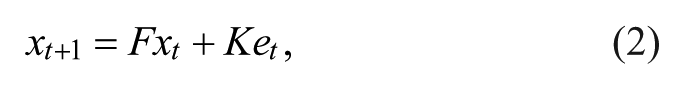
Analogous to the multivariate structural time series model, this study proposes a seasonally restacked multiseries structural time series model (M-STSM), in which the “multiseries” vector is formed by restacking the quarterly components that are split from the original quarterly series. As discussed above, the SSOE formulate is more general than its MSOE counterpart in terms of the parameter space and it generates better forecasts (de Silva, Hyndman, and Snyder 2010). Therefore, the SSOE scheme is adopted in this study. Following the notation introduced by Anderson and Moore (1979), the general form of the M-STSM can be formulated as

y_{t} = H x_{t} + e_{t}

x_{t + 1} = F x_{t} + K e_{t},

where $y_{t} = {(y_{1 t}, \dots, y_{4 t})}^{T}$ is a 4 × 1 vector of extracted quarterly components of the tourism demand series at time t. For instance, $y_{i t}$ refers to a time series of tourism demand in the ith quarter in the sample. Equations (1) and (2) are known as the measurement and transition equations, respectively. The structure matrix H and transition matrix F are typically fixed with dimensions of 4 × m and m × m respectively, and $x_{t}$ is the m × 1 vector of states. The innovations $e_{t}$ is a 4 × 1 vector that follows a normal distribution N(0, Σ). Following the suggestion by de Silva, Hyndman, and Snyder (2010), the covariance matrix Σ of innovations $e_{t}$ is assumed diagonal. K is an m × 4 impact matrix, in which the nonzero off-diagonal elements capture the interquarter associations at the latent component level. Through the impact matrix K, an innovation is allowed to influence other three series in addition to its own.

Based on the general form of the M-STSM, three special cases can be considered. The multiseries local trend model is specified as below:

y_{t} = μ_{t} + e_{t}

μ_{t} {_{+}}_{1} = μ_{t} + β_{t} + K_{μ} e_{t}

β_{t} {_{+}}_{1} = β_{t} + K_{β} e_{t},

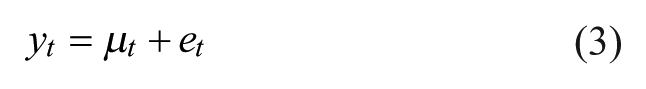
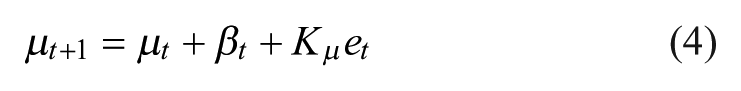
where $K_{μ}$ and $K_{β}$ are the impact matrices of 4 × 4 dimensions.

Based on the above multiseries local trend model, a multiseries damped local trend model consists of equations (3) and (4) with a slope having a damping factor Φ:

β_{t} {_{+}}_{1} = Φ β_{t} + K_{β} e_{t},

where the damping factor Φ is a 4 × 4 diagonal matrix. The absolute values of the diagonal elements are constrained to be less than 1 to ensure a stationary trend (Athanasopoulos and de Silva 2012).

Lastly, when the local trend $β_{t}$ is equal to 0, the transition equation (4) can be written as

μ_{t} {_{+}}_{1} = μ_{t} + K_{μ} e_{t},

where $K_{μ}$ is the impact matrix of 4 × 4 dimensions. Equations (3) and (7) are then referred to as the multiseries local-level model.

Model Estimation and Selection

The unknown parameters in an M-STSM can be estimated with a maximum likelihood method. In this study, the R program (R Core Team 2016) is used. We first evaluate the log-likelihood using a routine from the KFAS package (Helske 2016). The approach combines the exact diffuse initialization method (Koopman and Durbin 2003) with a sequential processing approach (Koopman and Durbin 2000) to reduce the computational costs of high-dimensional multivariate modeling. The results along with the initial values of parameters are then fed into an optimizer to search for optimal parameters that maximize the log-likelihood. As a commonly observed issue in multidimensional optimization, the process may only present local convergences instead of global ones. As a solution, a routine is used to start the optimizer multiple times from different sets of starting values and select the set that generates the largest log-likelihood as the estimates. An automatic model selection procedure is then deployed to select one of the aforementioned specifications based on the Akaike information criterion (AIC).

Forecasting Application and Data

The empirical case is based on Hong Kong inbound tourism demand from top 20 source markets, including Mainland China, Taiwan, Korea, USA, Japan, Macao, Philippines, Singapore, Australia, Malaysia, India, United Kingdom, Thailand, Indonesia, Canada, Germany, France, Italy, New Zealand, and Netherlands. The time series data for each source market are gathered and compiled from the Visitor Arrival Statistics (multiple editions) published by the Hong Kong Tourism Board. Each of the time series spans from the first quarter (Q1) of 1985 to the fourth quarter (Q4) of 2015.

To evaluate the forecasting performance of the models, up to the last 16 observations are withheld using an expanding window approach. In particular, the models are first estimated for each of the 20 source markets using the data up to 2011Q4, with the data spanning from 2012Q1 to 2015Q4 being held. A set of h = 1- to 16-quarter-ahead quarterly forecasts are generated. The estimation and forecasting process is carried on recursively until all available data are used up. For each round, the estimation period is extended by one quarter, and the models are re-estimated and then used for forecasting. In the end, this recursive process generates n = 17 – h sets of h-quarter-ahead forecasts, that is, 2,720 forecasts are generated in total (20 source markets and 136 forecasts per source market).

To perform quarterly forecasting with the M-STSM, a rolling sample approach can be used. Let s denote the sample size of the original time series, and let r be the remainder of s divided by 4. When r > 0, that is, the component series of $y_{t}$ are unbalanced, the first r observations in the original time series need to be deleted before splitting the series. Effectively, this process redefines the “year” in the sample. This is possible because an M-STSM captures associations between any four consecutive quarters that are not necessarily in the same calendar year. After the new multiseries data set is restacked, the M-STSM model can be estimated and used for forecasting.

The benchmark models introduced for the quarterly forecasting comparison include a SARIMA model and a univariate innovations ETS model given their generally sound performance in previous tourism studies. The forecast package (Hyndman and Khandakar 2008; Hyndman and Athanasopoulos 2014) is used to automatically select and estimate the ETS and SARIMA models.

The forecast accuracy is evaluated using two forecast error measures including the mean absolute percentage error (MAPE) and the mean absolute scaled error (MASE). The MAPE is one of the most commonly used measures in the literature. While the MASE is a scale-invariant and numerically stable measure that compares the mean absolute error (MAE) produced by the actual forecast against the one-step-ahead in-sample MAE from a seasonal naïve model (Hyndman and Koehler 2006; Hyndman and Athanasopoulos 2014).

Empirical Results

As shown in Figure 1, the inbound tourism demand for Hong Kong exhibits a diverse pattern of growth across the top 20 source markets. Over the last five years from 2011 to 2015, visitor arrivals from the major markets including Mainland China, Korea, and Macao have witnessed a drastic increase of more than 20% (Mainland China 63%). In contrast, the numbers for origins such as Indonesia, Japan, and Singapore have been declining. As a result of the outbreak of severe acute respiratory syndrome (SARS) in 2003, almost all inbound tourism flows clearly show a large dip particularly in the second quarter of the year. The impact of the Asian financial crisis around 1997–1998 can also be observed in many demand series but it is less prominent. Note that each inbound tourism flow is split into four component series in Figure 1. The gaps between component series indicate that seasonality is a common feature of Hong Kong inbound tourism demand across all markets. Visually, a tendency of co-movements among the four seasonal components is evident in most source markets. Further evidence is found through the Johansen cointegration test, which supports the application of the multivariate method to forecast these series jointly.

Figure 1.

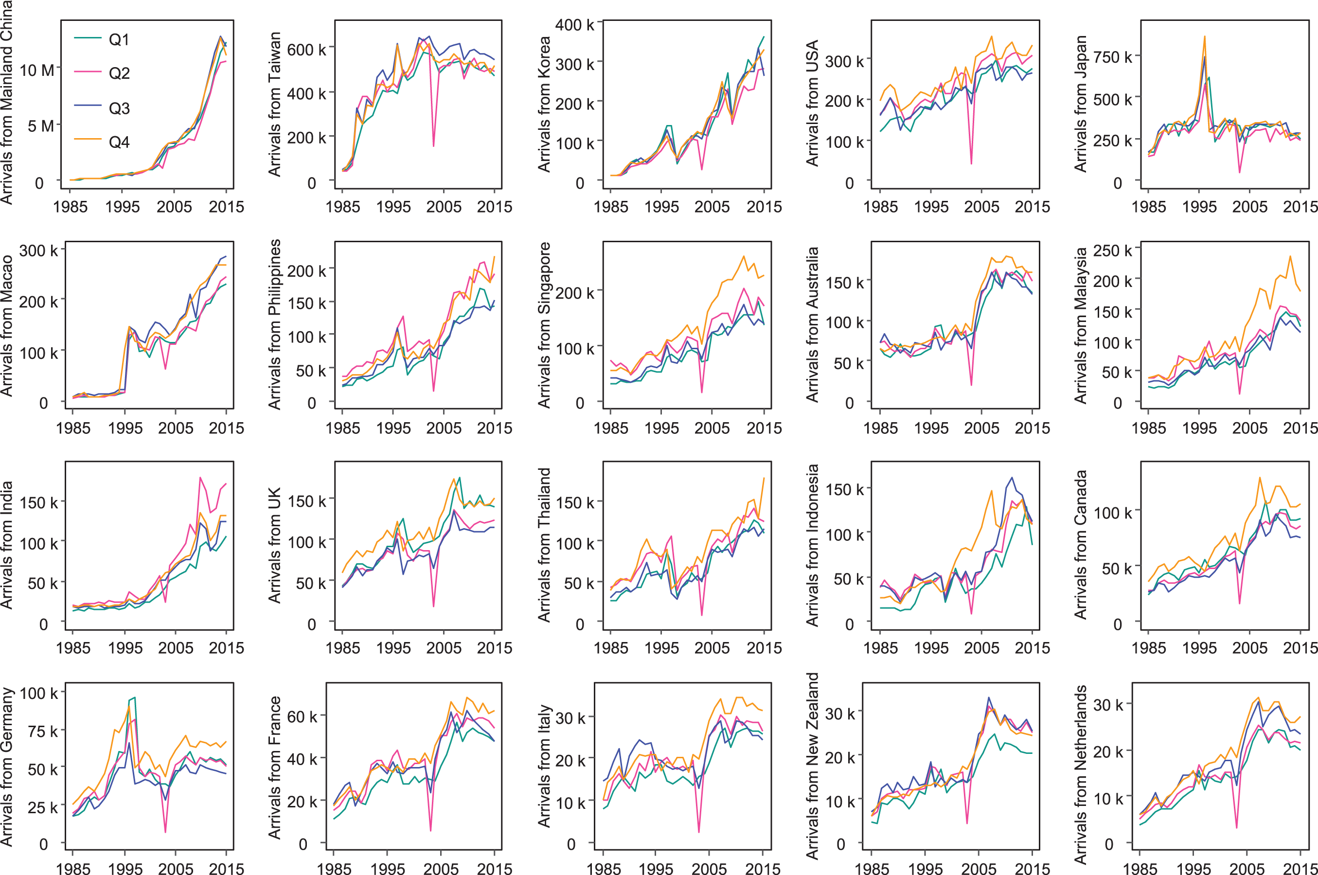
Seasonally extracted Hong Kong inbound visitor arrivals from the top 20 source markets.

After an M-STSM is estimated, a routine is used to check the model convergence as well as the standardized prediction errors. Among the 1,280 residual series generated in the estimation process (four component series for each of the 20 source markets, and 16 estimations per market), 1,235 (96.5%) have passed the Box-Ljung test, which reasonably satisfies the assumption of no autocorrelation.

Figures 2 and 3 display the results of average forecast errors across all forecast horizons. It is consistent for both MAPE and MASE that the M-STSM generates the most accurate forecasts throughout horizons 2 to 16, while the univariate ETS performs the best for one-quarter-ahead forecasts. The forecasts generated by the SARIMA model appear the least accurate relative to the other competing models. However, the differences in forecast accuracy among the models are only marginal until the forecast horizon h goes beyond 4, where the M-STSM outperforms the others with a clearer edge. Between the SARIMA and ETS methods, although the latter beats the former at most horizons (except for h = 12, 15, and 16), the gaps are not substantial. Overall, the proposed M-STSM performs the best, especially for the long-term forecasts.

Figure 2.

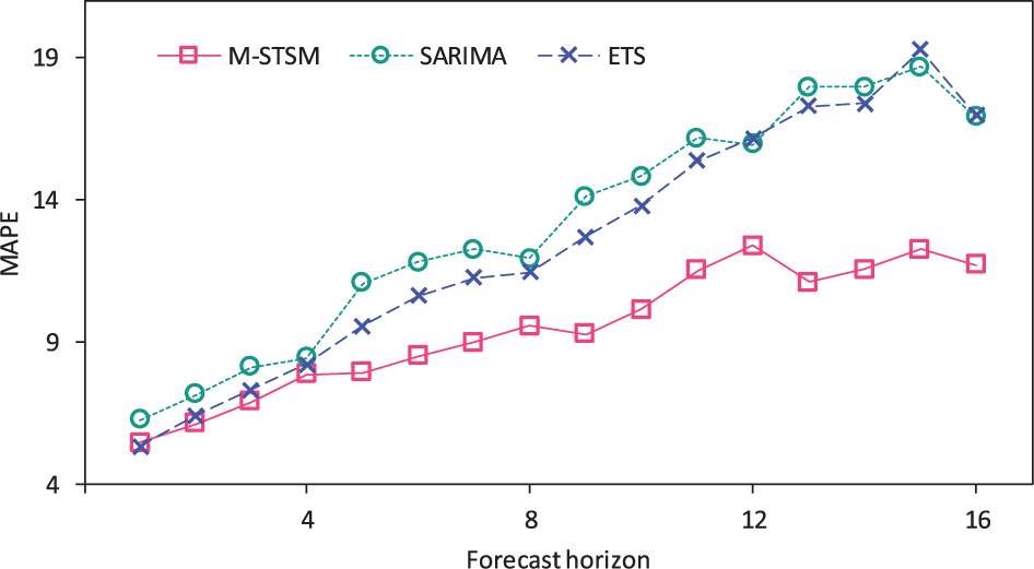
Average mean absolute percentage error (MAPE) by forecast horizon.

Figure 3.

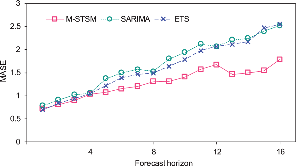
Average mean absolute scaled error (MASE) by forecast horizon.

In general, it is a desirable property of a time series model that more recent information is weighted more heavily than that obtained in the distant past (Hyndman et al. 2008). For seasonal forecasting, however, the information from the same season of previous years could be even more useful than that from previous seasons. In a study comparing quarterly forecasting performance of econometric models by Song et al. (2013), it has been found that a lag period of four quarters in the transition equation of a time-varying parameter (TVP) model captures seasonal fluctuations well in tourism demand. Underpinned by this rationale, an M-STSM built on the split series for each season is able to effectively use the information from the same season. Compared to the univariate method, the M-STSM may be less responsive to the most recent changes, but may be also less likely to overfit the data. Therefore, the restacking approach is expected to improve the long-term forecasting performance.

The quarterly forecasting performance and the average ranks of the competing models are presented in Table 1. Both error measures are averaged across all 20 source market cases by forecast horizon. In terms of the average ranks, the advantage of the ETS in the short-term forecasts (h = 1 to 4) becomes more evident. Yet the overall ranking throughout the horizons remains consistent with the previous finding that the M-STSM generates the most accurate forecasts, followed by the ETS model.

Table 1.

Average Accuracy of Quarterly Forecasts.

	MAPE			MASE
Horizon	M-STSM	SARIMA	ETS	M-STSM	SARIMA	ETS
1	5.45 [1.85]	6.25 [2.35]	5.32 [1.80]	0.72 [1.85]	0.78 [2.35]	0.69 [1.80]
2	6.12 [1.85]	7.14 [2.40]	6.42 [1.75]	0.80 [1.80]	0.91 [2.40]	0.84 [1.80]
3	6.91 [1.80]	8.11 [2.45]	7.32 [1.75]	0.90 [1.75]	1.02 [2.40]	0.94 [1.85]
4	7.87 [2.00]	8.43 [2.20]	8.20 [1.80]	1.03 [2.00]	1.05 [2.30]	1.04 [1.70]
5	7.93 [1.50]	11.06 [2.50]	9.57 [2.00]	1.07 [1.55]	1.37 [2.50]	1.22 [1.95]
6	8.52 [1.50]	11.80 [2.45]	10.63 [2.05]	1.15 [1.45]	1.50 [2.50]	1.39 [2.05]
7	8.98 [1.50]	12.25 [2.50]	11.26 [2.00]	1.20 [1.50]	1.57 [2.50]	1.46 [2.00]
8	9.57 [1.75]	11.94 [2.40]	11.47 [1.85]	1.31 [1.75]	1.53 [2.35]	1.49 [1.90]
9	9.28 [1.55]	14.13 [2.60]	12.72 [1.85]	1.31 [1.65]	1.80 [2.50]	1.64 [1.85]
10	10.13 [1.75]	14.84 [2.35]	13.80 [1.90]	1.41 [1.65]	1.94 [2.45]	1.79 [1.90]
11	11.52 [1.55]	16.18 [2.30]	15.36 [2.15]	1.57 [1.55]	2.12 [2.30]	1.98 [2.15]
12	12.38 [1.70]	15.95 [2.15]	16.17 [2.15]	1.67 [1.70]	2.07 [2.20]	2.07 [2.10]
13	11.09 [1.40]	17.98 [2.20]	17.31 [2.40]	1.46 [1.45]	2.21 [2.20]	2.11 [2.35]
14	11.56 [1.35]	17.96 [2.40]	17.41 [2.25]	1.50 [1.35]	2.24 [2.35]	2.17 [2.30]
15	12.26 [1.40]	18.68 [2.30]	19.30 [2.30]	1.54 [1.45]	2.40 [2.25]	2.47 [2.30]
16	11.70 [1.60]	16.91 [2.25]	16.98 [2.15]	1.79 [1.60]	2.52 [2.25]	2.55 [2.15]
1-16 Average	9.46 [1.55]	13.10 [2.35]	12.45 [2.10]	1.28 [1.55]	1.69 [2.35]	1.62 [2.10]

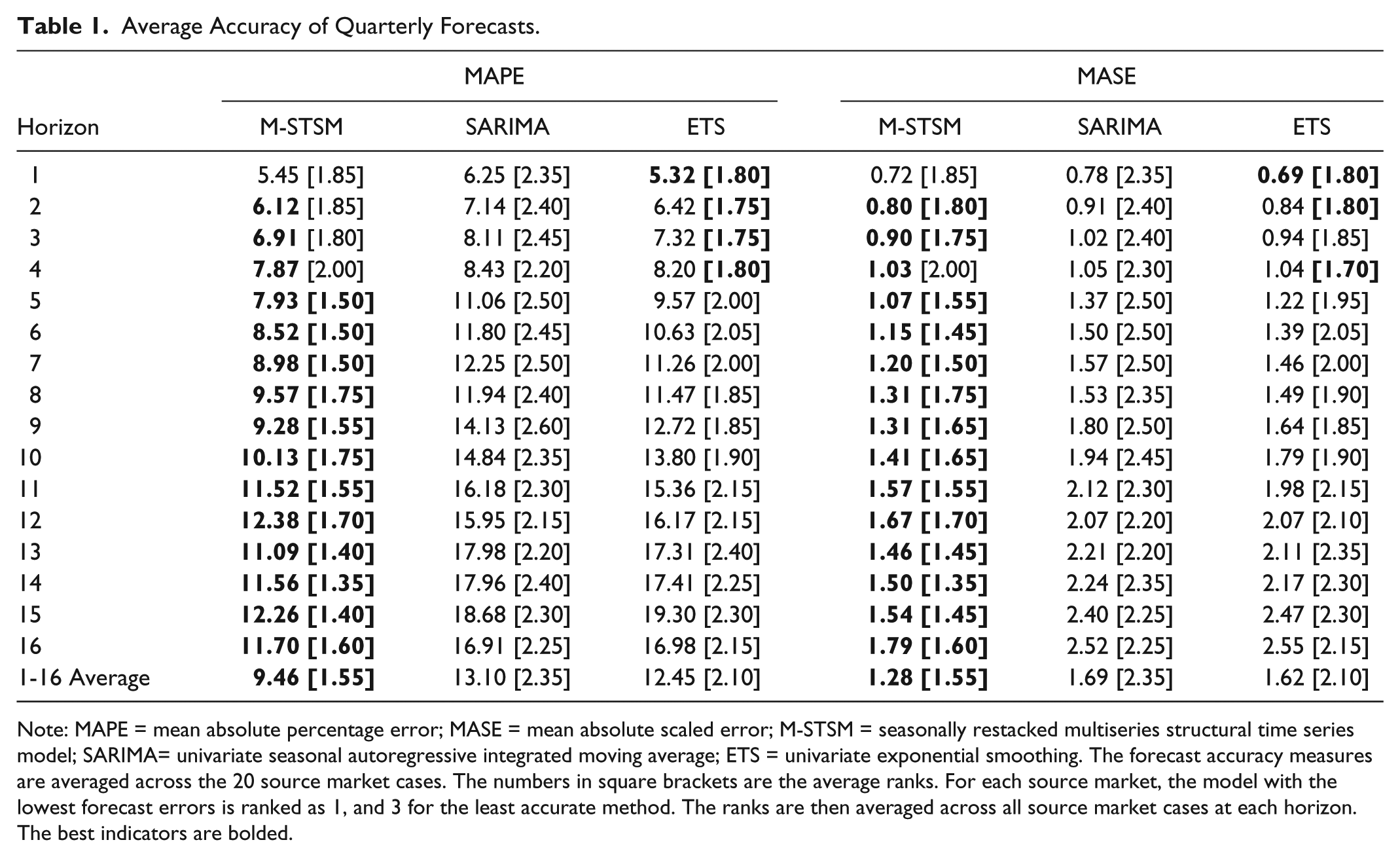
Note: MAPE = mean absolute percentage error; MASE = mean absolute scaled error; M-STSM = seasonally restacked multiseries structural time series model; SARIMA= univariate seasonal autoregressive integrated moving average; ETS = univariate exponential smoothing. The forecast accuracy measures are averaged across the 20 source market cases. The numbers in square brackets are the average ranks. For each source market, the model with the lowest forecast errors is ranked as 1, and 3 for the least accurate method. The ranks are then averaged across all source market cases at each horizon. The best indicators are bolded.

As far as each source market case is concerned (see Figures 4 and 5), the M-STSM forecasts most accurately in 60% of cases in terms of both MAPE and MASE averaged across all horizons, while the percentages of first ranks for the SARIMA and ETS methods are 15% and 25%, respectively. Compared to the SARIMA method, the ETS approach generally performs better. This is consistent with the finding of de Silva, Hyndman, and Snyder (2010) that even when an innovations ETS model is mathematically equivalent to an ARIMA process, the innovations method tends to produce better forecasts. By contrasting the MAPE and MASE measures, the results are generally consistent, but there are disparities in certain source market cases. As shown in Figures 4 and 5, the MAPE measures in the Mainland China models indicate an average performance among all the source markets. According to MASE, however, Mainland China is the case associated with the highest forecast errors. For a better understanding of the differences in the forecasting performance across source markets, it would be interesting to take a closer look at individual cases.

Figure 4.

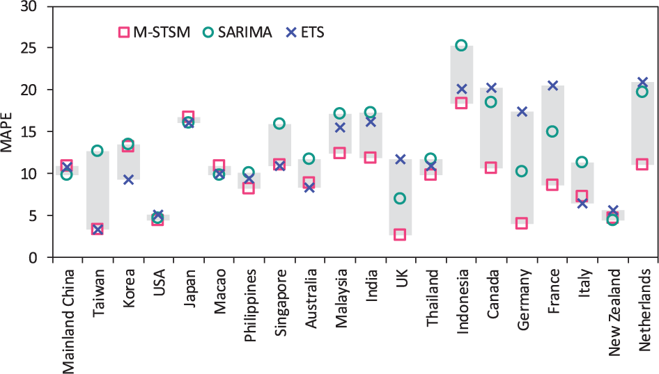
Average mean absolute percentage error (MAPE) by source market.

Figure 5.

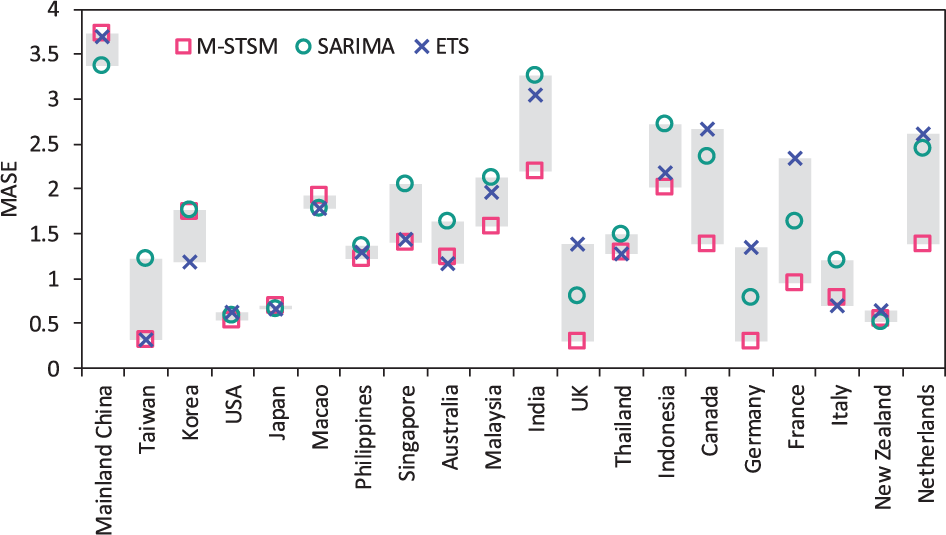
Average mean absolute scaled error (MASE) by source market.

Figures 6 –8 provide a closer insight into the forecast accuracy between the most and least accurate models. The dynamic forecasts (one set of h = 1- to 16-quarter-ahead forecasts) are presented in selected examples including Mainland China, Korea, and Germany. As shown in Figure 6, the SARIMA model outperforms the M-STSM in the case of Mainland China. However, because of the decline in tourism demand from Mainland China in 2015, both models overforecast tourist arrivals since the second quarter of 2015 as the estimation sample expanding toward the end of the series. This explains the relatively good performance of a seasonal-naïve model as indicated by the high MASE scores. In the case of Korea, the ETS model outperforms the M-STSM approach (see Figure 7). By comparing different model specifications of M-STSM, it is found that a local trend model would have generated better forecasts, while a local level model is selected based on the AIC. Nevertheless, AIC does correctly predict the forecasting performance in most cases, which is consistent with the finding of de Silva, Hyndman, and Snyder (2010). Similar to the majority of cases, the seasonal fluctuations of tourism demand from Germany are precisely captured by the M-STSM approach (see Figure 8). Although the seasonality is not explicitly specified in the M-STSM model, it is clear from the above benchmark results that the proposed M-STSM is an effective alternative for quarterly forecasting.

Figure 6.

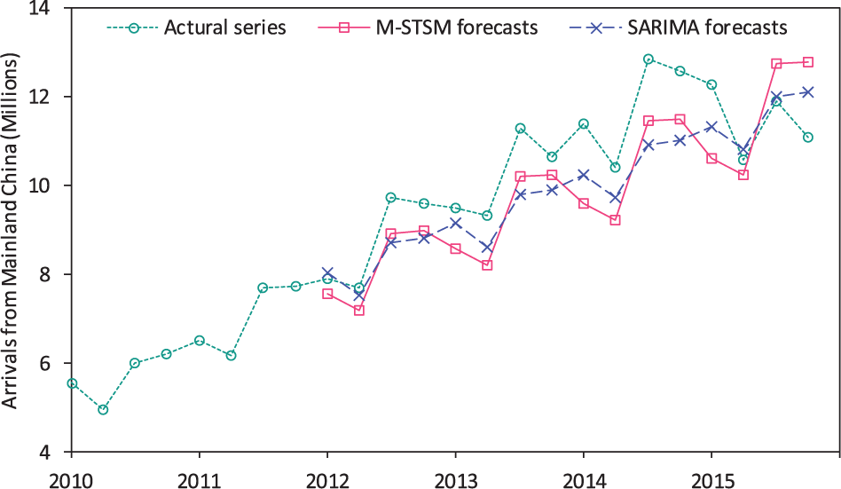
Dynamic forecasts for Mainland China, 2012Q1–2015Q4.

Figure 7.

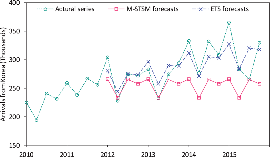
Dynamic forecasts for Korea, 2012Q1–2015Q4.

Figure 8.

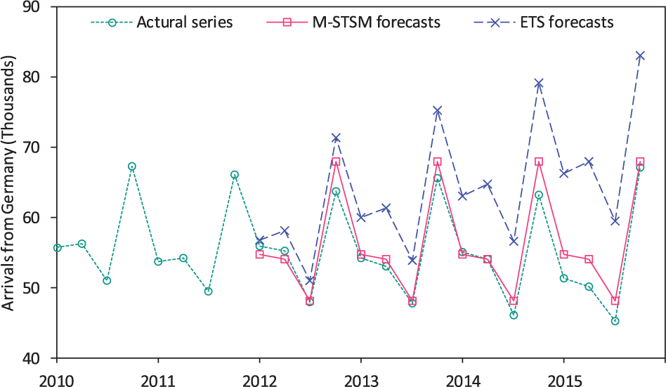
Dynamic forecasts for Germany, 2012Q1–2015Q4.

One of the motivations to apply the multivariate method is to use both backward and forward interquarter associations for forecasting. By comparing the performance of the M-STSM with the univariate models that are fitted to each of the component series separately, it has been found that the information of interquarter dependencies within a time series does contribute to the superior forecasting performance of the M-STSM. As described in the M-STSM formulation, the impact matrix K in equation (2) captures the interquarter associations of a time series. In particular, forward associations are specified for quarters 1, 2, and 3, and backward associates are modeled for quarters 2, 3, and 4. It would be therefore interesting to compare the forecasting performance by quarter, and contrast the results with the univariate models that are fitted to each of the component series. As shown in Table 2, the M-STSM forecasts quarter 1 and 2 component series more accurately relative to those for quarters 3 and 4. The results for the ARIMA and ETS are more mixed, but both perform the best in quarter 2 for both error measures averaged over all horizons and source markets. Compared to the univariate models, it is found that the forecast errors associated with the M-STSM are lower across all quarters with a percentage ranging from 16.23% to 45.24%. Therefore, it can be further concluded that both forward associations and backward associations across quarters are useful in improving forecast performance.

Table 2.

Average Accuracy of Forecasts by Quarter.

	MAPE			MASE
Quarter	M-STSM	ARIMA	ETS	M-STSM	ARIMA	ETS
Q1	4.94 [1.50]	5.84 [2.10]	6.32 [2.40]	0.78 [1.50]	0.87 [2.10]	1.01 [2.40]
Q2	7.45 [1.45]	9.14 [2.30]	9.78 [2.25]	1.17 [1.45]	1.37 [2.30]	1.57 [2.25]
Q3	9.05 [1.45]	12.21 [2.25]	12.30 [2.30]	1.47 [1.45]	1.93 [2.25]	2.08 [2.30]
Q4	11.19 [1.60]	15.67 [2.20]	16.56 [2.20]	1.55 [1.60]	2.24 [2.20]	2.85 [2.20]
Improvement,^a %
Q1	–	37.00	37.02	–	35.14	36.99
Q2	–	13.99	34.48	–	18.40	45.24
Q3	–	16.23	21.15	–	17.24	26.74
Q4	–	23.02	21.87	–	22.40	26.14

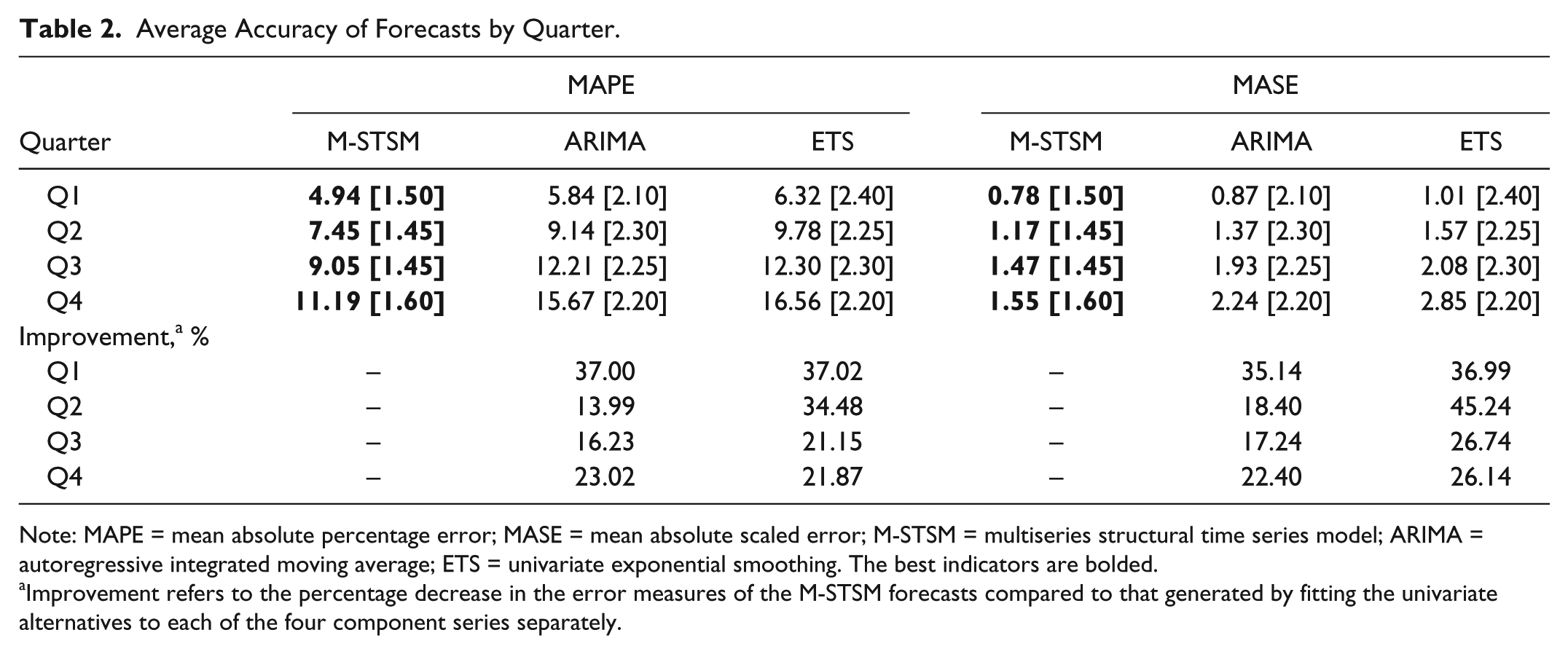
Note: MAPE = mean absolute percentage error; MASE = mean absolute scaled error; M-STSM = multiseries structural time series model; ARIMA = autoregressive integrated moving average; ETS = univariate exponential smoothing. The best indicators are bolded.

Improvement refers to the percentage decrease in the error measures of the M-STSM forecasts compared to that generated by fitting the univariate alternatives to each of the four component series separately.

Conclusion

This study continues to explore one of the most important issues in tourism demand analysis: seasonal tourism demand forecasting. Previous studies in this area normally model seasonality explicitly with an assumption of either a deterministic or stochastic nature of seasonality, or take certain seasonal adjustment techniques to deseasonalize a time series. Most often the modeling and forecasting exercises are based on univariate methods. The present study contributes to the literature in the following aspects. Firstly, this study adds to the limited literature of multivariate tourism demand forecasting by proposing a novel approach to forecasting seasonal tourism demand. Secondly and most importantly, this study exploits the interquarter dependencies within a time series to improve forecasting performance. It is the first attempt in the literature to apply a multivariate method in such an innovative setting, where potential misspecification and a source of forecast inaccuracy caused by modeling seasonality explicitly can be avoided. In the meanwhile, both backward and forward interquarter associations are taken into account in the multiseries model. The empirical results show that this information effectively improves the quarterly forecast accuracy. Lastly, the rolling sample forecasting strategy described in this study could be useful when dealing with unbalanced multiseries in general multivariate time series modeling and forecasting.

In the context of Hong Kong inbound tourist arrivals from the top 20 source markets, this study shows empirical evidence on the superior forecasting performance of the proposed multiseries approach over its univariate counterparts. This study suggests that the newly developed approach is an effective alternative to traditional methods of forecasting a seasonal series, especially for the long-term forecasts. To our knowledge, no such attempt has been made in other fields of forecasting. Therefore, the performance of this approach can be investigated in other contexts. Moreover, as the restacking approach could be applied to various multivariate models, it would be of interest to further examine the performance of other multivariate models with different formulations in future research.

Footnotes

Acknowledgements

The authors would like to acknowledge the financial support of the National Natural Science Foundation of China (Grant no. 71573289).

Declaration of Conflicting Interests

The author(s) declared no potential conflicts of interest with respect to the research, authorship, and/or publication of this article.

Author Biographies

Jason Li Chen is a lecturer in Tourism and Events in the School of Hospitality and Tourism Management at the University of Surrey. His research interests include tourism forecasting and quantitative methods in tourism studies.

Gang Li is a professor of Tourism Economics in the School of Hospitality and Tourism Management at the University of Surrey. His research interests are mainly in the area of economic analysis of tourism demand.

Doris Chenguang Wu is an associate professor in the Sun Yat-sen Business School of the Sun Yat-sen University, Guangzhou, China. Her research background is in tourism demand modeling and forecasting.

Shujie Shen is a senior lecturer in the Westminster Business School at the University of Westminster in the UK. Her research interests are in the areas of applied econometrics and tourism forecasting.

References

Akaike

1976. “Canonical Correlation Analysis of Time Series and the Use of an Information Criterion.” In System Identification, edited by Mehar

Lainiotis

, 27–96. New York: Academic Press.

Alleyne

2006. “Can Seasonal Unit Root Testing Improve the Forecasting Accuracy of Tourist Arrivals?” Tourism Economics 12:45–64.

Anderson

B. D. O.

Moore

J. B.

1979. Optimal Filtering. Englewood Cliffs, NJ: Prentice Hall.

Athanasopoulos

de Silva

2012. “Multivariate Exponential Smoothing for Forecasting Tourist Arrivals.” Journal of Travel Research 51 (5): 640–52.

Athanasopoulos

Hyndman

R. J.

Song

D. C.

2011. “The Tourism Forecasting Competition.” International Journal of Forecasting 27:822–44.

Athanasopoulos

Vahid

2008. “VARMA versus VAR for Macroeconomic Forecasting.” Journal of Business & Economic Statistics 26 (2): 237–52.

Bermúdez

J. D.

Corberán-Vallet

Vercher

2009. “Multivariate Exponential Smoothing: A Bayesian Forecast Approach Based on Simulation.” Mathematics and Computers in Simulation 79 (5): 1761–69.

Butler

R.W.

2001. “Seasonality in Tourism: Issues and Implications.” In Seasonality in Tourism, edited by Baum

Lundtorp

, 5–21. Oxford, UK: Pergamon.

Chatfield

1988. “The Future of Time-Series Forecasting.” International Journal of Forecasting 4:411–19.

10.

Cho

2001. “Tourism Forecasting and Its Relationship with Leading Economic Indicators.” Journal of Hospitality and Tourism Research 25 (4): 399–420.

11.

Claveria

Oscar

Monte

Enric

Torra

Salvador

. 2015. “Effects of Removing the Trend and the Seasonal Component on the Forecasting Performance of Artificial Neural Network Techniques.” IREA Working Paper 201503. University of Barcelona, Research Institute of Applied Economics.

12.

De Gooijer

J. G.

Hyndman

R. J.

2006. “25 Years of Time Series Forecasting.” International Journal of Forecasting 22:443–73.

13.

de Silva

Hyndman

R. J.

Snyder

R. D.

2009. “A Multivariate Innovations State Space Beveridge–Nelson Decomposition.” Economic Modelling 26:1067–74.

14.

de Silva

Hyndman

R. J.

Snyder

R. D.

2010. “The Vector Innovations Structural Time Series Framework: A Simple Approach to Multivariate Forecasting.” Statistical Modelling 10:353–74.

15.

du Preez

Witt

S. F.

2003. “Univariate versus Multivariate Time Series Forecasting: An Application to International Tourism Demand.” International Journal of Forecasting 19:435–51.

16.

Durbin

James

Koopman

Siem Jan

. 2012. Time Series Analysis by State Space Methods, 2nd ed. Oxford: Oxford University Press.

17.

Ghysels

Osborn

D. R.

2001. The Econometric Analysis of Seasonal Time Series. Cambridge, UK: Cambridge University Press.

18.

Goh

Law

2002. “Modeling and Forecasting Tourism Demand for Arrivals with Stochastic Nonstationary Seasonality and Intervention.” Tourism Management 23:499–510.

19.

González

Moral

1995. “An Analysis of the International Tourism Demand of Spain.” International Journal of Forecasting 11:233–51.

20.

González

Moral

1996. “Analysis of Tourism Trend in Spain.” Annals of Tourism Research 23:739–54.

21.

Harvey

A. C.

1989. Forecasting, Structural Time Series Models and the Kalman Filter. Cambridge, UK: Cambridge University Press.

22.

Helske

2016. “KFAS: Exponential Family State Space Models in R.” Journal of Statistical Software 78 (10): 1-39.

23.

Hinch

Jackson

2000. “Leisure Constraints Research: Its Value as a Framework for Understanding Tourism Seasonality.” Current Issues in Tourism 3:87–106.

24.

Hylleberg

1992. Modelling Seasonality. Oxford: Oxford University Press.

25.

Hyndman

R. J.

Athanasopoulos

2014. Forecasting: Principles and Practice. Heathmont, Australia: OTexts.

26.

Hyndman

R. J.

Khandakar

2008. “Automatic Time Series Forecasting: The Forecast Package for R.” Journal of Statistical Software 27 (3): 1–22.

27.

Hyndman

R. J.

Koehler

A. B.

2006. “Another Look at Measures of Forecast Accuracy.” International Journal of Forecasting 22 (4): 679–88.

28.

Hyndman

R. J

Koehler

A. B.

Ord

J. K.

Snyder

R. D.

2008. Forecasting with Exponential Smoothing: The State Space Approach. Berlin: Springer.

29.

Jones

R. H.

1966. “Exponential Smoothing for Multivariate Time Series.” Journal of the Royal Statistical Society, Series B (Methodological) 28 (1): 241–51.

30.

Kim

J. H.

1999. “Forecasting Monthly Tourist Departures from Australia.” Tourism Economics 5 (3): 277–91.

31.

Kim

J. H.

Moosa

2001. “Seasonal Behaviour of Monthly International Tourist Flows: Specification and Implications for Forecasting Models.” Tourism Economics 7:381–96.

32.

Kon

S. C.

Turner

W. L.

2005. “Neural Network Forecasting of Tourism Demand.” Tourism Economics 11:301–28.

33.

Koopman

S. J.

Durbin

2000. “Fast Filtering and Smoothing for Multivariate State Space Models.” Journal of Time Series Analysis 21 (3): 281–96.

34.

Koopman

S. J.

Durbin

2003. “Filtering and Smoothing of State Vector for Diffuse State-Space Models.” Journal of Time Series Analysis 24 (1): 85–98.

35.

Kulendran

King

1997. “Forecasting International Quarterly Tourism Flows Using Error Correction and Time Series Models.” International Journal of Forecasting 13:319–27.

36.

Kulendran

Witt

S. F.

2003a. “Forecasting the Demand for International Business Tourism.” Journal of Travel Research 41:265–71.

37.

Kulendran

Witt

S. F.

2003b. “Leading Indicator Tourism Forecasts.” Tourism Management 24:503–10.

38.

Kulendran

Wong

K. K. F.

2005. “Modelling Seasonality in Tourism Forecasting.” Journal of Travel Research 44:163–70.

39.

Leeds

2000. “Error Structures for Dynamic Linear Models: Single Source versus Multiple Source.” PhD diss., Department of Statistics, The Pennsylvania State.

40.

Song

Witt

S. F.

2005. “Recent Developments in Econometric Modelling and Forecasting.” Journal of Travel Research 44:82–99.

41.

Lim

McAleer

2001. “Monthly Seasonal Variations: Asian Tourism to Australia.” Annals of Tourism Research 28:68–82.

42.

Miron

J. A.

1994. “The Economics of Seasonal Cycles, in Advances in Econometrics.” In Sixth World Congress of the Econometric Society, edited by Sims

C. A.

, 213–51. Cambridge, UK: Cambridge University Press.

43.

Morzuch

B. J.

2005. “Evaluating Time-Series Models to Forecast the Demand for Tourism in Singapore.” Journal of Travel Research 43:404–13.

44.

Ord

J. K.

1988. “Future Developments in Forecasting: The Time Series Connexion.” International Journal of Forecasting 4:389–401.

45.

Ord

J. K.

Snyder

R. D.

Koehler

A. B.

Hyndman

R. J.

Leeds

2005. “Time Series Forecasting: The Case for the Single Source of Error State Space.” Monash Econometrics and Business Statistics Working Paper 7/05. Monash University, Department of Econometrics and Business Statistics.

46.

Osborn

D. R.

Harevi

Birchenhall

C. R.

1999. “Seasonal Unit Roots and Forecasts of Two-Digit European Industrial Production.” International Journal of Forecasting 15:27–47.

47.

Pegg

Patterson

Gariddo

P. V.

2012. “The Impact of Seasonality on Tourism and Hospitality Operations in the Alpine Region of New South Wales, Australia.” International Journal of Hospitality Management 31 (3): 659–66.

48.

Pfeffermann

Allon

1989. “Multivariate Exponential Smoothing: Methods and Practice.” International Journal of Forecasting 5: 83–98.

49.

Quenouille

M. H.

1957. The Analysis of Multiple Time-Series. New York: Hafner.

50.

R Core Team. 2016. R: A Language and Environment for Statistical Computing. Vienna, Austria: R Foundation for Statistical Computing.

51.

Rodrigues

P. M. M.

Gouveia

P. M. D. C. B.

2004. “An Application of PAR Models for Tourism Forecasting.” Tourism Economics 10:281–303.

52.

Snyder

R. D.

1985. “Recursive Estimation of Dynamic Linear Models.” Journal of the Royal Statistical Society, Series B (Methodological) 47 (2): 272–76.

53.

Song

Witt

S. F.

Athanasopoulos

2011. “Forecasting Tourist Arrivals Using Time-Varying Parameter Structural Time-Series Models.” International Journal of Forecasting 27:855–69.

54.

Song

Smeral

Chen

J. L.

2013. “Tourism Forecasting Using Econometric Models.” In Trends in European Tourism Planning and Organisation, edited by Buhalis

Dimitrios

Costa

Carlos

, 289–309. Bristol, UK: Channel View Publications.

55.

Turner

L. W.

Witt

S. F.

2001. “Factors Influencing Demand for International Tourism: Tourism Demand Analysis Using Structural Equation Modelling, Revisited.” Tourism Economics 7 (1): 21–38.