




Abstract
In this article, we sum up the literature on the study of Granger causality relationships between tourism and income using a meta-regression analysis. We conclude that the acceptance of the tourism-led growth hypothesis is likelier the higher the countries’ degree of tourism specialization and population size. However, neither these variables nor the level of economic development is relevant for the explanation of the probability of acceptance of the hypothesis of reverse Granger causality. Notwithstanding these results, we find that several features of the research design are associated with the acceptance of both hypotheses.
Introduction
Balaguer and Cantavella-Jordá (2002) are the pioneers of a line of research that studies the relationships between the development of international tourism demand and the expansion of the economic activity, under the aegis of what they called the “tourism-led growth” and the “growth-led tourism” hypotheses. The feature that distinguishes these studies is the application of Granger causality tests.
To date, this literature, which is the largest in the context of the study of the role of tourism in economic growth, has been summed up in three literature reviews: Brida et al. (2013), Pablo-Romero and Molina (2013), and Brida, Cortés-Jiménez, and Pulina (2016). In all of them, the authors conclude that the evidence available has favored the hypotheses above, namely the tourism-led growth hypothesis. They suggest, albeit without demonstrating it quantitatively, that the divergences in the conclusions obtained by the different studies can be explained by the differences in what concerns the sample periods analyzed, the variables chosen to represent the income and the tourism demand, the degree of sophistication of the econometric analysis and the degree of tourism specialization of the analyzed countries. In this article, we intend to use meta-regression analysis to test the role of these factors in the explanation of the discrepancies between the existing results.
Our approach is driven by empirical considerations. We intend to take stock, in the form of a quantitative synthesis, of almost a decade and a half of research. Since the pioneering contribution of Balaguer and Cantavella-Jordá (2002), several studies came into light and several conclusions were obtained, often contradictory even for the same country under analysis. In fact, although most of the studies validate the presence of some type of Granger causal relationship between tourism and income, the contradictions found in the literature are large enough so it cannot be stated that there is a consensus.
The general proposition tested throughout our study is that the probability of acceptance of each one of the Granger causal hypotheses between tourism and income is a function of two sets of variables. The first set includes variables associated with the research design, namely, the features of the study and the data, the type of variables chosen to represent the income and the tourism demand, and the features of the statistical analysis. The second set relates to some of the variables that are likely to explain the genuine variation of the empirical effect, that is, the genuine variation in the probability of acceptance of the causal hypotheses under analysis. This second set refers to the economic variables already suggested by the aforementioned literature (Brida et al. 2013; Brida, Cortés-Jiménez, and Pulina 2016; Pablo-Romero and Molina 2013), namely, the level of economic development, the degree of tourism specialization, and the size of the analyzed countries.
For the sake of clarity, it should be noted that it is not our purpose to test the hypotheses of Granger causality between tourism and income. In this article, we aim to analyze the role of the aforementioned sets of variables in the explanation of the differences between the results of the Granger causality tests between tourism and income in the studies available. That is, we seek to shed light on why results differ from one study to another.
The work developed here differs from the previous narrative reviews because of its quantitative approach to the literature by means of a meta-regression analysis. In this sense, we intend to add to the literature an empirical evaluation of the importance of the factors deemed to be valuable to the explanation of the differences between the results of the existing studies. By doing so, we intend to add to the explanation of why results differ sometimes even for the same country analyzed in different studies. Our approach is inspired by a distinct but related meta-analysis paradigm, namely, the meta-regression analysis developed by T. D. Stanley and his coauthors (Stanley and Doucouliagos 2012; Stanley et al. 2013). However, we do not directly address issues related to publication bias, nor is this our intention. In this sense, our methodological approach is identical to the one followed by Peng, Song, and Crouch (2014).
The remainder of this article is divided into five more sections. In the following section, we put forth a brief review of the literature available, explaining how the meta-analyzed studies were selected and presenting an overview of their main conclusions. In the third section, we present our methodology of meta-regression analysis. The sources and the data that allowed the construction of the meta-dependent and meta-independent variables, as well as the respective descriptive statistics, are presented in the fourth section. The meta-regression analyses themselves, and the discussion of the results, are carried out in the next section. The final section presents our main conclusions, together with some new avenues for future research.
Overview of the Literature
Our study fits into the context of the broader literature focused on the empirical analysis of the relationships between tourism development and economic growth. Within this literature, there are two major strands. The first strand concerns the cross-country studies with panel data whose theoretical foundations lie on the theories of exogenous and endogenous economic growth (Solow 1956; Mankiw, Romer, and Weil 1992). These studies typically analyze several countries for a relatively shorter number of years, and Castro-Nuño, Molina-Toucedo, and Pablo-Romero (2013) summed up a comparable selection of studies within this literature by means of a classical meta-analysis. Their findings reveal the presence of a positive elasticity between gross domestic product (GDP) and tourism, even though its magnitude varies according to the methodologic procedures employed in the original studies. A larger selection of this type of studies is included in the narrative and nonquantitative literature review presented by Brida, Cortés-Jiménez, and Pulina (2016), but obviously, contributions do not cease to come to light. In this sense, Beladi et al. (2019), Chiu and Yeh (2017), and Zuo and Huang (2018) constitute three very recent and innovative contributions.
The second strand of the literature analyzes the Granger causal relationships between tourism development and economic growth, following the path initiated by Balaguer and Cantavella-Jordá (2002). The usual analysis consists of a country case study. However, as more complete databases have emerged, with longer and comparable time series, and as the necessary statistical tools have evolved, we have witnessed the emergence of a growing number of panel data analysis based on the use of cointegration and Granger causality techniques. Brida et al. (2013), Pablo-Romero and Molina (2013), and Brida, Cortés-Jimenez, and Pulina (2016), whose contributions we describe below, present very complete narrative reviews of this strand of the literature.
Because of the aforementioned evolution of databases and econometric techniques, this line of research is not only the most prolific, but it is also constantly evolving. As such, at the time of the writing of this text, some other interesting and valuable contributions emerged, namely, the ones by Antonakakis et al. (2019), Liu and Song (2018), and Wu and Wu (2018), among others. Our study is a meta-analysis, by means of multiple linear regression techniques, of this second research strand, and it is innovative because of the quantitative nature of our approach.
As it is certainly obvious by now, our study also differs from the previous meta-analysis of Castro-Nuño, Molina-Toucedo, and Pablo-Romero (2013) because of the methodology, scope, and theoretical basis of the studies we included in our analysis. They analyze cross-country studies based on panel data studies and grounded on the exogenous and endogenous theories of economic growth. We focus on country case studies (more detail on this later) based on time series data and Granger causality tests and supported by the theoretical arguments we will describe now.
The literature we examine addresses the analysis of two fundamental hypotheses. These are (1) the tourism-led growth hypothesis, according to which the expansion of tourism demand Granger causes the increase of the economic activity; and (2) the growth-led tourism development hypothesis (or hypothesis of reverse Granger causality), which corresponds to the opposite of the previous one and postulates that the expansion of the economic activity Granger causes the development of the tourism activity. Additionally, there is the hypothesis of bidirectional Granger causality, which corresponds to the simultaneous verification of the two previous hypotheses and means, therefore, that the development of tourism and the expansion of economic activity Granger cause each other.
In the context of this literature, the empirical validation of the different hypotheses has different implications for economic policy. The empirical validation of the first hypothesis suggests that the allocation of more resources to activities directly linked to tourism might exert positive effects on economic growth. The validation of the second hypothesis indicates that the development of the tourism activity depends on a drag effect exerted by other more dynamic sectors, to which a higher volume of resources should be channeled. The validation of the third hypothesis, suggesting that tourism is complementary to the remainder of the economic system, points to a balance in the allocation of resources between tourism and the remaining economic activities. On the other hand, the rejection of the first hypothesis means that the resources and strategies that may have been directed at promoting and developing the tourism sector may not have been as effective as one would expect.
To our knowledge, ours is the first quantitative review of the literature on the study of Granger causality between tourism and income. Nevertheless, there are already three narrative reviews available: the ones by Brida et al. (2013), Pablo-Romero and Molina (2013) and Brida, Cortés-Jiménez, and Pulina (2016). In the first study, the authors list the 50 articles published to date and exhaustively describe their main results. Relevant to our study is the fact that Brida et al. (2013) have concluded that the differences between the results obtained by the different studies may be associated with differences regarding the variables chosen to represent tourism and income. The authors also suggest that the results may differ according to the econometric techniques applied or to the degree of tourism specialization of the analyzed countries.
Brida, Cortés-Jiménez, and Pulina (2016) extend the review to 95 articles, although several of them relate to panel data (often without a country-by-country breakdown) or to cross-sectional data analyses. On the other hand, not all the studies reviewed by them based on time series data apply Granger causality tests. With relevance to us, the conclusions of Brida, Cortés-Jiménez, and Pulina (2016) corroborate those of Brida et al. (2013) with respect to the sensitivity of the results in terms of the differences regarding the variables that represent tourism and income, to the econometric techniques applied, and to the degree of tourism specialization of the analyzed countries. The authors also stress that there is an apparent bias in the economic profile of the countries whose results are available, which seem to be heavily dependent on tourism. Because of that it is not possible to generalize the conclusion that the tourism-led growth hypothesis is universal.
Pablo-Romero and Molina (2013) review 62 empirical studies based on time series analysis. Like the two previous narrative literature reviews, they conclude that most of the studies favor the presence of Granger causal relationships between tourism and income. They also stress “the relevance of the country’s specialization in tourism in order for tourism to affect growth” and the fact that “the small size of the country seems to broaden the effect on economic growth caused by tourism.”
In our meta-analysis, we will evaluate the validity of the assertions presented by the aforementioned authors. That is, we will evaluate the extent to which the measurement of the variables, the methodologies of testing for Granger causality, the degree of tourism specialization, and the geographic dimension of the countries are helpful in the explanation of the differences between the results obtained by the studies. We will also add the economic development level, to analyze the extent to which the acceptance of each of Granger causality hypotheses depends on this variable.
Methodology
Size of the Empirical Effect
In the usual meta-regression analyses, the empirical effect under analysis is a regression coefficient or—mainly due to problems of heteroscedasticity—the t statistic associated with that same coefficient or a transformation of that statistic (Stanley and Doucouliagos 2012). However, when the meta-analysis refers to the results of Granger causality tests, this option is no longer available because the associated statistics result from F or chi-square tests and not from t tests. For the results of these tests to be used as empirical effects, it is necessary to convert them into a common metric with a common distribution and statistical properties that are suitable for regression analysis (Bruns, Gross, and Stern 2014; Stanley 2005).
The first solution would be to convert the results of the Granger causality tests into discrete nominal variables that would assume the values 1, 2, 3, etc., depending on the hypotheses or alternatives under analysis. This was the approach chosen by Sebri (2015) in his meta-regression analysis of the studies concerning the Granger causal relationships between the consumption of renewable energies and economic growth.
The second solution is the transformation of the probabilities of significance of the original test statistics into standardized normal variables, as suggested by Abramowitz and Stegun (1964) and acknowledged by Stanley (2005). The solution adopted by Bruns, Gross, and Stern (2014) falls within this line and consists of converting the probabilities of significance of the test statistics associated with the F and chi-square tests through a
Model and Variables
We aim to estimate the parameters of several versions of the linear meta-regression model given by

where
Table 1 depicts the total set of variables. The empirical effect corresponds to the symmetric of the probit transformation of the probability of significance associated with the results of the F or chi-square tests to the relevant hypothesis.
Variables Included in the Meta-regression Analyses.

Note: The empirical effects and the variables of the vector
Vector
The second, third, and fourth sets of variables assess the role of aspects related to the specification of the models, namely, the frequency of the data (Annual, Quarterly, and Monthly) and the proxies chosen to represent the income of the visited country (Real GDP, Real GDP real per capita, Growth Rate of GDP, and Other income) and the respective inbound tourism demand (Tourism Receipts, Tourism Arrivals, and Other Tourism). The different choices are likely to influence the results of the Granger causality tests, even though in unknown directions.
The fifth and sixth sets include variables that capture the role played by methodological options regarding the cointegration (Johansen, ARDL, Other cointegration, and Cointegration not tested) and Granger causality analyzes (VECM, VAR, TYDL, and Other tests of causality). It is not possible to anticipate how the different options influence the magnitude of the empirical effect, but the literature reviews available suggest the existence of differences.
The meta-independent variables included in vector
The literature available reveals that, in general, the presence of Granger causality between tourism and income appears to be more common in countries that are less developed, more specialized in tourism, and smaller, hence the inclusion of variables that represent these three aspects (Brida, Cortés-Jiménez and Pulina 2016; Pablo-Romero and Molina 2013). Thus, on the one hand, we want to test the hypothesis that countries starting from lower levels of economic development, higher degrees of tourism specialization, and lower demographic size have higher empirical effects associated with the Granger causality tests from tourism to income. On the other hand, we want to test the hypothesis that countries with higher initial levels of economic development have higher empirical effects associated with the Granger causality tests from income to tourism.
The variable that represents the level of Economic development results from the ratio between the real GDP per capita of each country in the first year of the time series analyzed, and the real per capita GDP of the United States that same year. This variable allows direct comparisons between the initial levels of economic development of countries whose starting points (i.e., whose first years of the sample) differ from each other. Taking the United States as a developed country that has grown steadily over the period covering all available starting points (1954 to 2009), we can state that a country whose level of development in year t was equal to 0.4 (for example) started from a higher level of economic development than another country whose level of development in the year t+k, with k integer, was equal to 0.3.
To measure the degree of Tourism specialization, we chose tourism receipts as a percentage of total exports of services in the first year of each time series analyzed. The numerator corresponds to the expenditure on goods and services purchased by foreign visitors at the destination during the stay (less than one year), whether for personal or business purposes. Our choice is in line with the alternatives of measurement of the degree of tourism specialization suggested, for example, by Piotrowski, Arezki, and Cherif (2009), although the share of tourist revenues in total GDP in total exports are also common choices. In comparison with these two alternatives, we believe that the indicator we have chosen is preferable because it reduces the endogeneity that would arise from the use of GDP or total exports in the denominator. Furthermore, our choice was conditioned by the availability of directly comparable data for the range of the analyzed countries.
The Country size is assessed through the respective population size, a usual choice in the theoretical literature on the role of the scale effects on economic growth (e.g., Dinopoulos and Thompson 1999; Howitt 1999; Jones 1995), as well as in the corresponding empirical literature (e.g., Brau, Lanza, and Pigliaru 2007; Easterly and Kraay 2000; Laincz and Peretto 2006; Streeten 1993). As we are seeking to establish comparisons between countries at different points in time, it is necessary to remove the effect associated with the trend of this variable. We did so by calculating the percentage of the population of each country in the first year of the sample analyzed, in relation to the world population in that same year. Therefore, this variable measures the share of each country in the world population, in each year of the sample.
Estimation Issues
Because of the nature of the meta-dependent variable (a probit transformation) and the existence of several observations associated with a single author, the appropriate method of estimation is the ordinary least squares with robust standard errors in clusters (Stanley and Doucouliagos 2012, 2015 ). The vector of the estimated coefficients of the meta-regression is given by
The model is initially estimated with all the meta-independent variables and then goes through a process of successive elimination of the variables whose estimated coefficients present probabilities of significance (i.e., p values) higher than 10%, within the spirit of the general-to-specific methodology of the London School of Economics (e.g., Hendry and Nielsen 2007). The application of this type of procedure in meta-regression analyses is suggested by Stanley et al. (2013). In our case, we eliminate the statistically least significant variables in each estimation round. That is, in each round of estimation, we eliminate the variable with the highest probability of significance until we have a final model composed only of variables with statistically significant coefficients for significance levels of 10% or lower (Stanley et al. 2013). The application of this strategy in the various subsamples allows us to obtain parsimonious models with the highest possible explanatory power and to test the sensitivity and robustness of the results.
This set of procedures is done twice, once for the empirical effect associated with the results of the tests for the hypothesis of Granger causality from tourism to income, and another for the empirical effect associated with the results of tests for the hypothesis of reverse causality. At all stages, all the models are subject to a battery of statistics and diagnostic tests related to the goodness of fit and the quality of the models, to the normality and homoscedasticity of the residuals of estimation, and to the presence of specification errors. In this sense, R2 indicates the adjusted coefficient of determination, F(k-1,n-k) corresponds to the value of the robust F statistic in clusters of the test to the null hypothesis of joint nonsignificance of the estimated coefficients of meta-regression, where k is the number of estimated regression coefficients and n is the number of observations, and White corresponds to the value of the test statistic of the null hypothesis of absence of heteroscedasticity.
As is well known, rejection of the null hypothesis of homoscedasticity renders the OLS estimators inefficient (although they maintain their consistency), which, in turn, invalidates the results of the statistical inference. However, this possibility is partly mitigated by the fact that we have calculated robust standard errors in clusters, which were intended to correct the most likely pattern of heteroscedasticity. However, where there is evidence of the presence of heteroskedasticity, it is always necessary to take extra care in the interpretation of the results.
The rejection of the null hypothesis of normality of the residuals of estimation has no consequences on the consistency or efficiency of the estimators. In large samples of hundreds of observations or more, the assumption of normality is not even necessary, since the Central Limit Theorem ensures the convergence of the distribution of the disturbance terms to normality. The problem arises in small samples. In these cases, the violation of the assumption of normality implies being more conservative in carrying out tests of statistical significance or in the construction of confidence intervals, leading us to the preference for significance levels of 1% rather than the usual 5% or the “relaxing” 10%. The nonrejection of the null hypothesis of normality of the residuals is, obviously, always reassuring.
In the tables presented in the fifth section, below each coefficient of meta-regression, we placed the value of the robust standard error in clusters, being that we considered 11 clusters, one for each set of observations in which at least one of the authors emerges repeatedly.
Because of the chosen method of estimation (OLS with robust standard errors in clusters), the F statistic is not calculated as usual. On the contrary, it involves complex matrix notation, from which sometimes singular or quasi-singular matrices result. In these cases, the software does not return the value of this statistic, situations in which we inserted the acronym NA (“not available”) in the corresponding position in the tables.
Data
Selection of the Studies
The relevant papers report empirical studies that analyze the dynamic relationships between tourism demand and income by means of tests of Granger causality. The identification of the studies was carried out through the Scopus and Google Scholar databases, which resulted in 123 potentially relevant studies. For our purposes, we were interested only in papers with the following characteristics: empirical analyses at the national level (i.e., countries or autonomous territories); time series data or panel data provided that, in the latter case, results were broken down by country; the level of real income of the visited country and the corresponding level of inbound tourist demand within the range of the variables analyzed; and the application of Granger causality tests based on the Engle-Granger approach, VAR models, VEC models, or ARDL models. The exclusion of papers that do not fall into these features serves two purposes. On the one hand, the chosen papers aim to ensure the highest possible comparability among the studies. On the other hand, they intend to reduce the potential influence of spurious regressions or other econometric errors that could compromise the quality of our analysis.
The application of the criteria of inclusion and exclusion resulted in the 55 studies presented in Table 2. It should be noted that our selection of works is practically coincident with those of the narrative reviews analyzed in the previous section, which is not only comforting but also allows direct comparisons between our conclusions and the conclusions of those reviews.
Studies Included (in Chronological Order).

Of the 55 studies selected, the majority (91%) refers to articles published in peer-reviewed journals, and the remaining are unpublished working papers. The inclusion of the latter is justified by the procedures of systematic reviews of the literature suggested by Cooper (1982, 2010) and by Cooper and Hedges (2009) and offer us the possibility to assess whether the empirical effects of unpublished studies differ significantly from the empirical effects of published studies.
Descriptive Statistics
Our full sample includes 78 empirical effects on Granger causality from tourism to income and 74 empirical effects on Granger causality from income to tourism. These empirical effects were collected from 51 studies (Table 1) and included the analysis of 42 countries (Table 3). From the 55 initial studies, we excluded four because of the lack of information regarding some of the meta-independent variables described hereafter. Our final sample size is large enough to guarantee statistically consistent results, in addition to being comparable or even superior to the sample size of several well-known studies that also apply meta-regression methods (see the references discussed in Stanley and Doucouliagos 2012).
Countries and Number of Empirical Effects Collected.
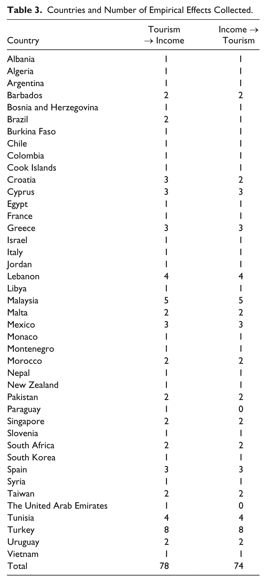
The sample is overrepresented by countries with medium or low levels of economic development, which had, in fact, already been noticed by Brida, Cortés-Jiménez, and Pulina (2016). However, this overrepresentation has nothing to do with our study selection strategy because the studies we selected match almost exactly those included in the available narrative reviews. Rather, this overrepresentation is a direct consequence of the researchers’ choices.
Table 4 depicts the variable’s descriptive statistics and offers an overall perspective of the data. It is noted that all variables have variability amenable to be exploited. Most of the empirical effects are related to published studies (93.6%) that analyzed annual data (69.2%). Usually, the income and tourism variables are measured, respectively, by means of levels of real GDP (51.3%) and tourism receipts (62.8%). The Johansen method is the preferred strategy of analysis of cointegration (47.4%), and the Granger causality testing, through the estimation of a vector error correction model (VECM), is the most usual choice (44.9%). The analysis of Table 4 also reveals that the average country is quite less developed than the United States and presents a rather high level of dependence on tourism.
Descriptive Statistics.
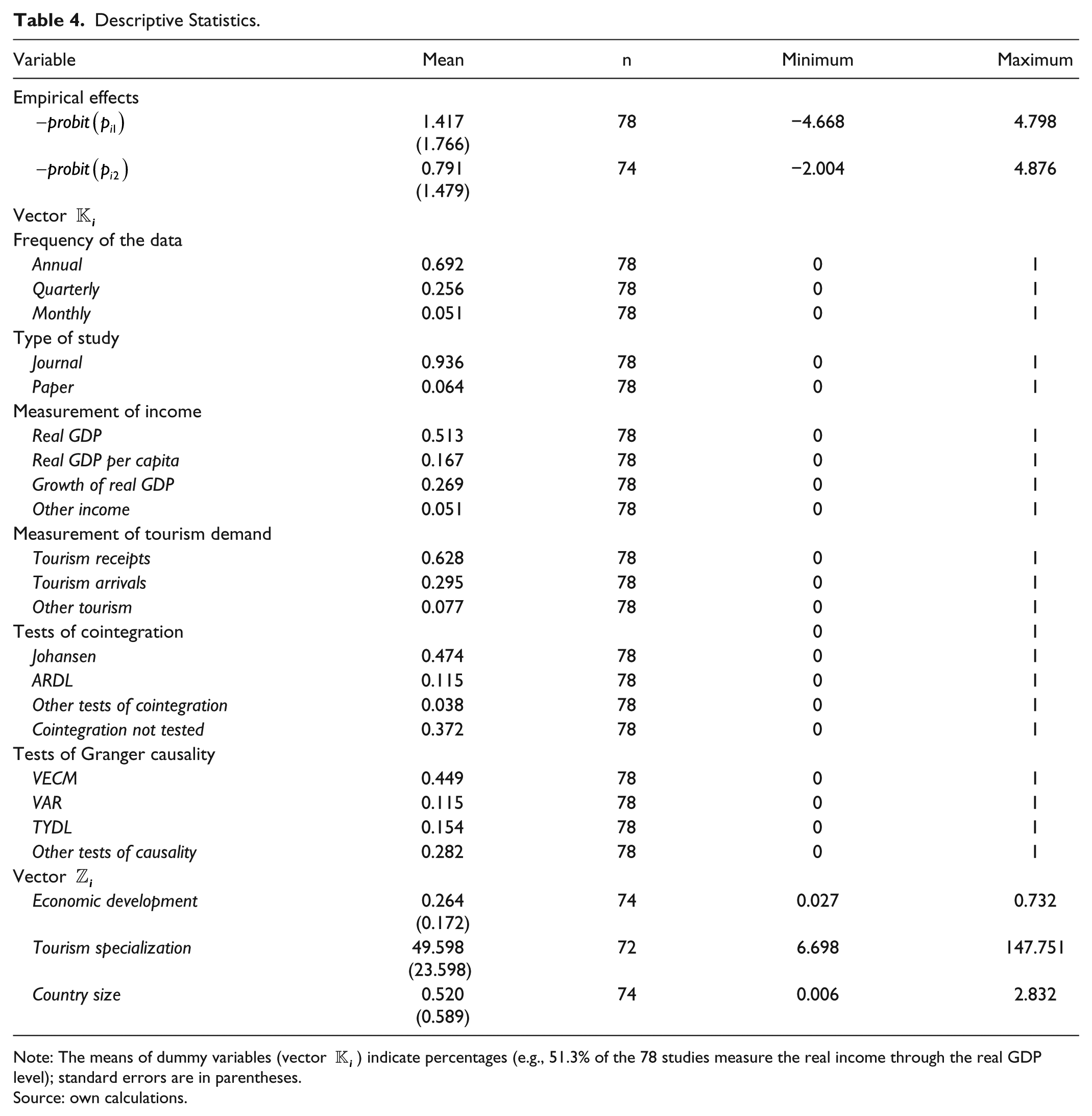
Note: The means of dummy variables (vector
Source: own calculations.
Coefficients of Correlation
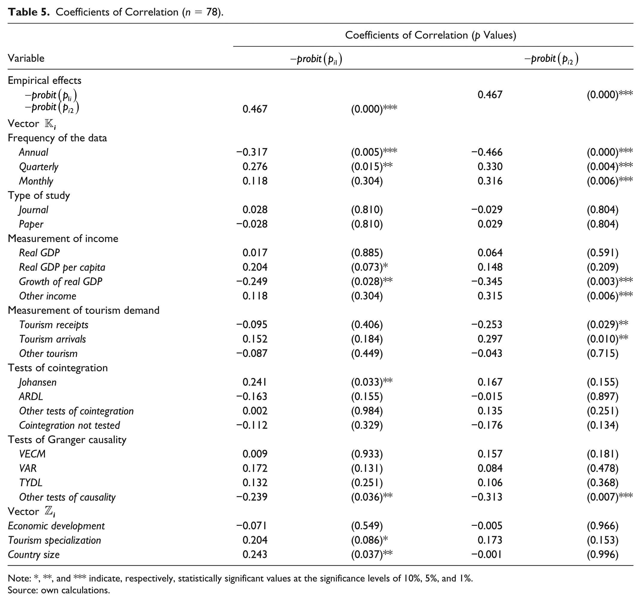
Table 5 presents the coefficients of correlation between each of the empirical effects and the remaining variables. We find that the two empirical effects are positively and significantly correlated with each other (r = 0.47; p value < 0.01).
Coefficients of Correlation (n = 78).
Note: *, **, and *** indicate, respectively, statistically significant values at the significance levels of 10%, 5%, and 1%.
Source: own calculations.
We also find that the values of the empirical effects tend to be statistically and significantly smaller when the data analyzed by the original studies are annual, when the proxy for income is the growth rate of real GDP, and when the Granger causality tests applied are other than the usual ones. However, concerning these last two variables, Real GDP growth and Other tests of causality, the results of the correlations presented are strongly conditioned by the work of Tugcu (2014), which provides 21 of the 78 observations available and is the only one that measures the product through the growth rate of real GDP. As such, in the following section, in all meta-regression analyzes, we present the estimation results with a dummy variable for the work of Tugcu (2014).
The choices concerning the measurement of the tourism demand (by means of the Tourism arrivals or by means of the Tourism receipts) are correlated with the empirical effect
With regard to the variables intended to explain the heterogeneity of the empirical effect, there are two positive and statistically significant correlations that are noteworthy, namely, between the degree of specialization in tourism and between the geographic dimension and the empirical effect
We calculated the coefficients of correlation between the different groups of meta-independent dummy variables, whose results are available under request. As expected, there are several statistically significant correlations between pairs of variables. Therefore, the inclusion of different groups of variables in the same meta-regression would generate problems of perfect or near perfect multicollinearity, making it more difficult to interpret the results of estimation. Because of this, the meta-regressions presented in the following section will never include different groups of this type of variables in the same meta-regression.
We also calculated the coefficients of correlation between the continuous meta-independent variables. The only statistically significant correlation is the one between the degree of Tourism specialization and the Country size: we find that the countries with higher levels of tourism specialization tend to be smaller in terms of the size of their population (r = −0.33; p value < 0.01). The combination with the fact that the correlation between the empirical effect associated with Granger causality from tourism to income (
Results
This section puts forward the estimation results of several versions of model (1). We present one table for each of the cases,
Meta-regressions for the Results for the TLG Hypothesis.

Notes: *, **, and *** indicate, respectively, statistically significant values at the significance levels of 10%, 5%, and 1%. The even columns correspond to the final models resulting from the reduction process performed from the initial models estimated in the odd columns. TLG = tourism-led growth.
Source: own calculations.
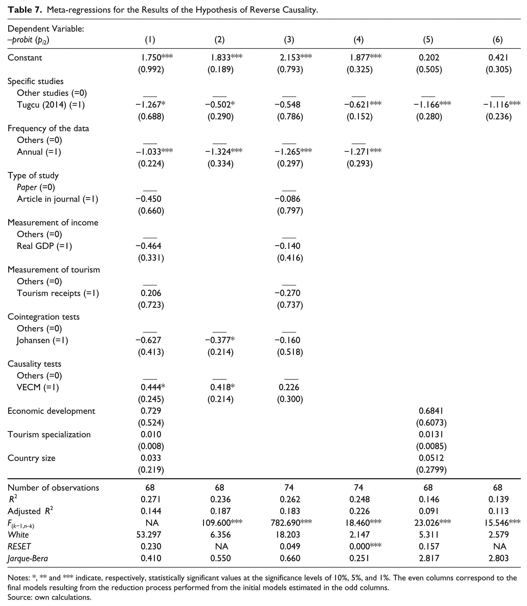
Meta-regressions for the Results of the Hypothesis of Reverse Causality.
Notes: *, ** and *** indicate, respectively, statistically significant values at the significance levels of 10%, 5%, and 1%. The even columns correspond to the final models resulting from the reduction process performed from the initial models estimated in the odd columns.
Source: own calculations.
We begin with the empirical effect associated with the Granger causality from tourism to income. The main results are presented in columns 1 and 2 of Table 6. The estimated coefficients of the reduced model (column 2) are statistically significant at significance levels of 1% or less. This is very important because the null hypothesis of normality of the residuals is rejected in all the estimated meta-regressions presented in Table 6. The statistically significant coefficients relate to the variables Tugcu (2014) (p value = 0.006), Tourism specialization (p value = 0.002), and Country size (p value = 0.001).
Columns 3 and 4 repeat the approach, but now just considering the variables of vector
The results presented in Table 6 reveal that the probability of acceptance of the tourism-led growth hypothesis is lower when income is measured through a growth rate, as the dummy for Tugcu (2014) captures this effect too. Conversely, it is also shown that the same probability is higher the higher the degree of tourism specialization and the population size of the country under analysis.
In Table 6, as well as in the remaining tables, the coefficient of determination value is a bit low. However, one must bear in mind that a meta-regression analysis is a mere statistical exercise, not necessarily an economic one, backed up with a solid theory. Our aim is not to explain an economic phenomenon but rather to explain the variability of the results found in a strand of literature. Actually, it would be quite odd if factors not taken into account by the original studies could explain a significant portion of that variability. As such, our focus lies on the statistical significance of the variables deemed to contribute to the explanation of the heterogeneity of the empirical effects, independent of the statistical models’ goodness of fit.
We now look into the analysis of the empirical effect associated with Granger causality from income to tourism, whose main results are presented in Table 7. The estimation of the complete model (column 2) reveals that the relevance of the variable Tugcu (2014) decreases considerably because it is only statistically significant for a confidence level of 10%. However, unlike in Table 6, in this table the null hypothesis of normality of the residuals is never rejected.
In columns 3 and 4, we consider only the variables of vector
In order to test the sensitivity and robustness of the results obtained, we estimated the same models, complete and reduced, without the dummy for Tugcu (2014) and without the data taken from this study. The reason for the considerations made about the work of Tugcu (2014) is related to two facts. On the one hand, the 21 observations taken from it account for a significant proportion (26.9%) of the total observations available, which could lead to bias or distortion of the conclusions. On the other hand, it is the only study where the variable that represents income is a growth rate (in this case, of the real GDP) and not a level, which also, for this same reason, can be a source of bias or distortion. Despite our fears, the results obtained based on these considerations confirm those presented above and are available on request. We prefer the versions with the dummy for Tugcu (2014) because it turned out to be statistically significant and it increased the explanatory power of the models in terms of adjusted coefficient of determination. Therefore, the inclusion of this variable adds to the improvement of the statistical quality of the models.
Finally, we evaluated the role played by each of the secondary categories of the variables of vector
Meta-regressions for the Results for the TLG Hypothesis: Further Results.

Notes: *, ** and *** indicate, respectively, statistically significant values at the significance levels of 10%, 5%, and 1%. In (a) the variable was removed because of its perfect correlation (r = 1.000) with the dummy variable representative of Tugcu (2014); (b) the variable was removed because of its almost perfect correlation (r = 0.968 and p value <0.001) with the dummy variable of Tugcu (2014). TLG = tourism-led growth.
Source: own calculations.
Meta-regressions for the Results of the Hypothesis of Reverse Causality: Further Results.
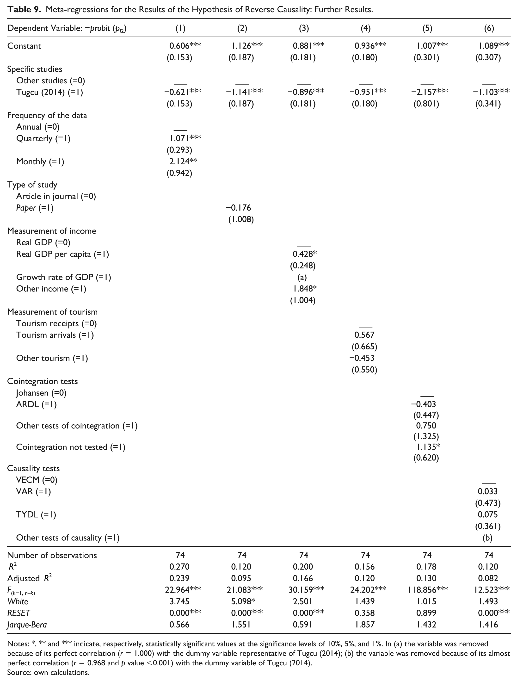
Notes: *, ** and *** indicate, respectively, statistically significant values at the significance levels of 10%, 5%, and 1%. In (a) the variable was removed because of its perfect correlation (r = 1.000) with the dummy variable representative of Tugcu (2014); (b) the variable was removed because of its almost perfect correlation (r = 0.968 and p value <0.001) with the dummy variable of Tugcu (2014).
Source: own calculations.
In Table 8, the coefficient of the dummy variable for Tugcu (2014) is always negative and statistically significant, for significance levels below 1% or 5%. The coefficient of the variable Monthly, in column 1, is positive and statistically significant for a significance level of less than 1% (p value < 0.001), as well as the coefficients of the variables Other income (positive) in column 3 (p value = 0.003) and ARDL (negative) in column 4 (p value < 0.001). Moreover, the variable Real GDP per capita (column 3) has a positive and statistically significant coefficient, for a significance level of 5% (p value = 0.035).
In Table 9, the variable Tugcu (2014) presents a statistically significant coefficient for a significance level of 1% in all specifications. Furthermore, the variables Quarterly and Monthly (column 1) are the only ones whose estimated coefficients are positive and statistically significant for a significance level of 5%.
Therefore, the evidence presented herein tell us that some methodological choices are amenable to contribute to obtaining higher empirical effects associated to the Granger causality tests in both directions. The highlight goes to the frequency of the data, where the choice of higher frequencies leads to larger empirical effects, and to the variable chosen to measure income, where the measurement of income through a growth rate instead of a level of real GDP leads to lower empirical effects.
Regarding these two tables, 8 and 9, we also estimated alternative versions of the models without the dummy variable or the data related to the work of Tugcu (2014). The results obtained, which are available on request, do not contradict those presented here.
Conclusions
In this study, we presented a quantitative review of the literature concerned with the study of the hypotheses of Granger causality between tourism and income. For this purpose, we used an exploratory meta-regression analysis.
We concluded that the tourism-led growth hypothesis is more likely to be accepted in the case of countries that are more specialized in tourism and that have larger populations. If the first of these conclusions is hardly surprising, the same cannot be stated about the second one. Indeed, it represents a contradiction both regarding the conclusions of the theories on the role of tourism in economic growth and the conclusions of the available literature reviews. Future studies should confirm or disprove these empirical regularities.
Interestingly, we concluded that neither the level of economic development nor the degree of specialization in tourism or the population size are helpful in explaining the heterogeneity of the conclusions associated with the Granger causality from income to tourism.
However, our results allowed us to conclude that, in general, the probability of acceptance of any of the causal hypotheses is higher when the income is measured in levels (rather than through a growth rate) or when quarterly or monthly data (rather than annual data) are used. The application of specific methodologies for Granger causality testing is also associated with higher or lower probabilities of acceptance of both causal hypotheses. The overall reading is that if the authors of the empirical papers or the editors of the journals have a preference for statistically significant results, the chances of publication decrease if the income is measured by means of a growth rate of income, rather than a level of income, and increase if the frequency of the data is monthly or quarterly, rather than annual.
When we compare our conclusions with those of the available narrative reviews, we find both similarities and differences. On the side of similarities, we find the role of the degree of tourism specialization and the sensitivity of the results to aspects such as the choice of the variables to represent the income.
On the side of the differences, we have the already-mentioned allusion to the role of country size. If a narrative review, namely, Pablo-Romero and Molina (2013), points out that the countries’ small size can contribute to accentuating the effect of tourism on economic growth, our meta-regression analysis has led us to the opposite conclusion. We found confirmation of one of the conclusions of our simple correlations: that the population size and the degree of tourism specialization might be correlated with each other but, at the same time, they seem to be independent determinants of the tourism-led growth effect. However, it could also be the case that our findings are not really in contrast with the previous literature. Since the sample of countries available is mainly composed of small countries, maybe the positive relationship between the country size and the relevant empirical effect holds only below a certain threshold of the country size. That is, perhaps the positive relationship between the acceptance of the tourism-led growth hypothesis and the population size presents nonlinearities. Only future research can dissipate these doubts.
In addition to the already presented avenues for future research, we believe that the presence of statistically significant correlations between several characteristics of the research design and the results of the Granger causality tests require further investigation. In this regard, it is necessary to question the presence of problems of publication bias in order to find out whether the authors of the studies or the editors of the journals really prefer the presentation and publication of results tending to the validation of at least one of the hypotheses of Granger causality analyzed.
There is another limitation in the literature worthy of attention, especially in the light of the results we put forth herein. Considering that both the degree of tourism specialization and the population size seem to be relevant for the explanation of the tourism-led growth hypothesis, future studies theoretically should back up those relationships. That is, neither the available theories nor the arguments behind the tourism-led growth hypothesis are able to explain or predict the empirical facts we found. As such, our results are amenable, we hope, to trigger fruitful paths for the empirical and theoretical literature on the relationships between tourism development and economic growth.
Footnotes
Acknowledgements
We would like to thank the anonymous reviewers for their helpful and insightful comments that greatly contributed to the improvement of the article.
Declaration of Conflicting Interests
The author(s) declared no potential conflicts of interest with respect to the research, authorship, and/or publication of this article.
Funding
The author(s) received no financial support for the research, authorship, and/or publication of this article.
