Forecasting Tourism Demand with an Improved Mixed Data Sampling Model

Abstract

Search query data reflect users’ intentions, preferences and interests. The interest in using such data to forecast tourism demand has increased in recent years. The mixed data sampling (MIDAS) method is often used in such forecasting, but is not effective when moving average (MA) dynamics are involved. To investigate the relevance of the MA components in MIDAS models to tourism demand forecasting, an improved MIDAS model that integrates MIDAS and the seasonal autoregressive integrated moving average process is proposed. Its performance is tested by forecasting monthly tourist arrivals in Hong Kong from mainland China with daily composite indices constructed from a large number of search queries using the generalized dynamic factor model. The forecasting results suggest that this new model significantly outperforms the benchmark model. In addition, comparing the forecasts and nowcasts shows that the latter generally outperforms the former.

Keywords

tourism demand forecasting MIDAS search query data generalized dynamic factor model nowcasts

Introduction

The perishable nature of the tourism industry makes accurately forecasting tourism demand an important task for tourism- and hotel-related decision makers. It is impossible to store unfilled airline seats and unsold hotel rooms. Therefore, accurate demand forecasts can help tourism practitioners make business decisions, such as those concerning scheduling, staffing, and pricing. In addition, policy makers in tourist destinations need accurate forecasts to formulate tourism development policies, such as tourism infrastructure investments.

Traditional tourism demand forecasting studies have often used historical tourism demand and macroeconomic data. However, macroeconomic data, such as GDP and CPI, are usually delayed and may take several weeks or months to be published. The rapid development of information technology and the Internet has given rise to massive-scale and readily available data (Kambatla et al. 2014). Such data often reflect users’ intentions and can serve as early indicators of various activities. For example, search queries have been used for various forecasting purposes, such as unemployment claims (Choi and Varian 2012), influenza epidemics (Ginsberg et al. 2009), and housing prices and sales (L. Wu and Brynjolfsson 2015).

Search query data have also gained popularity in forecasting tourism demand. Tourists use search engines to look for travel information on weather, transportation, hotels, attractions, travel guides, and other tourists’ opinions (Fesenmaier et al. 2011). These web search behaviors are recorded and reflect users’ intentions, preferences, and interests. Therefore, they can be valuable predictors of tourism demand. Although the use of search query data in tourism demand forecasting is relatively new, interest in this area has increased rapidly in recent years. Search query data have often been aggregated and converted into the same frequency as tourism demand variables in previous studies because they are often sampled at a higher frequency (Choi and Varian 2012; X. Li et al. 2017; Pan, Wu, and Song 2012; Rivera 2016; Yang et al. 2015). This can lead to information loss and poor forecasting performance because high frequency information is not used (Ghysels, Sinko, and Valkanov 2007). Bangwayo-Skeete and Skeete (2015) were the first to introduce mixed data sampling (MIDAS) for tourism demand forecasting. They found that MIDAS performed better in forecasting monthly tourist arrivals using weekly Google Trends data in most forecasting exercises, whereas its performance was poor in other exercises.

Compared with common benchmark models, such as the seasonal autoregressive integrated moving average (SARIMA) model, traditional MIDAS models often involve autoregressive (AR) components and are unable to incorporate moving average (MA) dynamics. Indeed, they are not effective when the underlying data include MA dynamics. In fact, in a recent study, Foroni, Marcellino, and Stevanovic (2019) showed that MA components emerged in a MIDAS model in which the low-frequency variable was the result of temporal aggregation. They investigated the effect of neglecting MA components in the forecasts and found that including MA components improved the forecasting performance of their Monte Carlo simulations and application to US macroeconomic variables. In this study, the same idea is introduced to tourism demand forecasting, and the relevance of MA components is investigated in this context. In addition, Foroni, Marcellino, and Stevanovic (2019) focused on forecasting macroeconomic variables and did not consider seasonal ARMA components. As tourism demand often exhibits strong seasonality, it is important to account for seasonality in the modeling process. Moreover, Foroni, Marcellino, and Stevanovic (2019) arbitrarily determined the orders of AR and MA components in MIDAS models. Doing so may yield a higher probability of model misspecification. To overcome these problems, a new model that integrates the MIDAS and SARIMA processes is proposed. This new model is an extension of traditional MIDAS models and is able to accommodate seasonal and nonseasonal ARMA components. The features of the MIDAS and SARIMA models are especially relevant in the tourism demand forecasting context. The mixed frequency aspect of the new model provides a more efficient way to utilize high-frequency search query data. Furthermore, its seasonal and nonseasonal ARMA components capture important characteristics of tourism demand. In this study, the effectiveness of the model is investigated by forecasting monthly tourist arrivals in Hong Kong from mainland China, with daily composite indices constructed from a large number of search queries using the generalized dynamic factor model (GDFM). Previous studies have focused on forecasting or nowcasting tourism demand. In contrast, this study is the first to conduct a comparison analysis of forecasts and nowcasts. Such a comparison may be particularly useful for decision makers who need frequent updates to make more accurate forecasts. When forecasting tourism demand, traditional macroeconomic data, such as income level in the origin country and relative price level in the destination country, are often incomplete and subject to revision for the current and most recent periods. However, search query data are readily available on a daily and even hourly basis. They are especially useful in a nowcasting framework, which can enable more timely tourism demand forecast updates when new information becomes available. For example, timely and improved updates of nowcasts of demand are very valuable in hotel revenue management, which involves dynamic pricing.

The remainder of this article is organized as follows. The second section reviews the relevant literature. The third section presents the data and the construction of the search query index. The fourth section discusses the details of the models and their estimation results. The fifth section presents the forecasting and nowcasting results. The final section concludes.

Literature Review

Tourism Demand Forecasting

Tourism demand forecasting is a well-established research area. The three main types of modeling techniques include noncausal time series, econometric, and artificial intelligence (AI)–based methods.

Traditional time series models include Naïve 1 models (no change), Naïve 2 models (constant growth rate), exponential smoothing models, and simple AR models (Song and Li 2008; D. C. Wu, Song, and Shen 2017). They are often used as benchmarks in tourism forecasting studies. Autoregressive integrated moving average (ARIMA) models and SARIMA models are the most commonly used models, depending on the frequency of the time series. Various extensions of the ARIMA model have also been used in the literature. For example, Chu (2009) introduced an autoregressive ARMA (ARARMA) model and a fractionally integrated ARMA (ARFIMA) model to forecast tourist arrivals in nine destinations in the Asia-Pacific region and found that the ARFIMA model outperformed the SARIMA and ARARMA models. Similarly, Assaf, Barros, and Gil-Alana (2011) used several models based on fractional integration to forecast tourist arrivals in Australia, confirming that they outperformed the standard ARIMA and SARIMA models.

Structural time series (Turner and Witt 2001) and generalized autoregressive conditional heteroskedastic (Divino and McAleer 2010) models have also been widely used in the tourism literature. In recent years, more advanced time series models have been used to generate better forecasting performance than traditional time series models, such as innovations state space models for exponential smoothing (ETS; Athanasopoulos et al. 2011), singular spectrum analysis (SSA) models (Hassani et al. 2017), and time-varying parameter structural time series models (Song et al. 2011). Decomposition methods, such as SSA, empirical mode decomposition (Yahya, Samsudin, and Shabri 2017), and ensemble empirical mode decomposition (Zhang et al. 2017), have gained much popularity in recent years and have demonstrated good forecasting performance. These techniques have been used in univariate time series forecasting settings (Hassani et al. 2017; Hassani et al. 2015; Silva et al. 2019) and causal time series forecasting settings (X. Li and Law 2020).

Unlike noncausal time series models, econometric models can analyze the relationship between tourism demand and its key determinants, and the information can be used to provide policy recommendations. Several important factors affecting tourism demand have been identified in the literature, such as tourist income, tourism prices in a destination relative to those of the country of origin, tourism prices in competing destinations, and real exchange rates (Song and Li 2008; D. C. Wu, Song, and Shen 2017).

Spurious regression is often present in traditional regression analysis. Several modern econometric models have been introduced in tourism modeling and forecasting, such as the autoregressive distributed lag model (Song, Gartner, and Tasci 2012), the error correction model (Goh 2012), the vector autoregressive (VAR) model (Wong, Song, and Chon 2006), the time-varying parameter model (Page, Song, and Wu 2012), the almost ideal demand system model (G. Li, Song, and Witt 2006), and the Bayesian VAR model (Gunter and Önder 2015; Wong, Song, and Chon 2006). Numerous studies have concluded that econometric models perform better (Song, Witt, and Jensen 2003), but some have confirmed that time series models outperform econometric models in predicting tourism demand (Athanasopoulos et al. 2011).

In addition to time series and econometric methods, a variety of AI-based methods have been introduced in the tourism forecasting literature. The dominant model is the artificial neural network (ANN) model. It consists of several layers, each of which can contain multiple neurons. The ANN model is a nonparametric and data-driven method that can be used to model nonlinear relationships. It is also the most frequently used AI-based method in tourism demand forecasting studies (Claveria, Monte, and Torra 2015; Law et al. 2019; S. Sun et al. 2019). Other AI-based methods used to forecast tourism demand include the support vector machine model (Chen et al. 2015; Hong et al. 2011), the fuzzy system model (Aladag et al. 2014), the rough set model (Goh, Law, and Mok 2008), and gray theory (X. Sun et al. 2016).

Although various methods have been introduced and applied in the literature, there is a consensus that no model can outperform other models consistently under all conditions (Song and Li 2008). Using a meta-analysis, Peng, Song, and Crouch (2014) showed that their data characteristics and study features, such as demand measure, data frequency, and origin–destination pairs, affected the forecasting accuracy of tourism demand.

Forecasting with Search Query Data

People often search for information online, and their search behavior reflect their consumption preferences and decision-making processes (Du, Hu, and Damangir 2014; Ghose, Ipeirotis, and Li 2014). Search query data can serve as a powerful predictor to improve forecasting accuracy. Thus, forecasting using search query data has gained popularity in a number of research areas.

For example, Ginsberg et al. (2009) investigated a large number of Google search queries to track influenza-like illnesses; ultimately, their method improved early detection. Since then, researchers have explored the usefulness of search query data for forecasting unemployment rates (Askitas and Zimmermann 2009), consumer consumption (Vosen and Schmidt 2011), stock markets (Bordino et al. 2012; Da, Engelberg, and Gao 2011), automobile sales (Du and Kamakura 2012), and house prices and sales (L. Wu and Brynjolfsson 2015).

In recent years, forecasting tourism demand using search engine data has also attracted attention. For example, Choi and Varian (2012) used Google Trends data for the first 2 weeks of each month to predict the number of visits to Hong Kong in a given month. Pan, Wu, and Song (2012) chose five related Google search queries to forecast demand for hotel rooms in Charleston, US, improving forecasting performance by including search query data. Pan and Yang (2017) used Google search engine queries and website traffic data to forecast hotel demand in Charleston and found that their forecasts were more accurate when they included both data sources. Rivera (2016) pointed out that Google Trends data differ each week because the data are constructed as a relative volume and come from a periodic sample of queries. Therefore, he proposed using a dynamic linear model and treated Google Trends data as a representation of an unobservable process. In addition, the association between hotel demand and Google Trends data can be better understood when the data are downloaded on multiple occasions. Yang et al. (2015) used Google Trends and the Baidu Index, which represents the absolute volume of the chosen search queries, to forecast the number of visitors to a province in China. They found that although the data from both search engines improved forecasting accuracy, the Baidu Index performed better. X. Li et al. (2017) used the GDFM to construct the composite index from a large number of Baidu search queries to forecast tourist arrivals in Beijing. They showed improved forecasting performance using the GDFM compared with another dimension reduction method, principal components analysis. Recently, studies have also used ANNs to model the relationship between tourism demand and search query data. S. Sun et al. (2019) used Google and Baidu search data to forecast tourist arrivals in popular destinations in China, showing better forecasting performance when using the kernel extreme learning machine model. Similarly, Wen, Liu, and Song (2019) used the Baidu Index to forecast tourist arrivals in Hong Kong from mainland China, using a newly proposed hybrid model integrating the ARIMA and ANN models. They found that the hybrid model outperformed component models. Law et al. (2019) applied a deep learning approach to forecast tourist arrivals in Macau using search query data. They showed that the deep learning approach significantly outperformed the support vector regression model and the traditional ANN model.

MIDAS Regressions

Time series data are often collected at different frequencies, but most models require variables to be converted to the same low frequency. During this process, the potentially valuable information contained in high-frequency variables is smoothed and lost. To tackle this problem, Ghysels, Santa-Clara, and Valkanov (2004) used MIDAS regressions to directly estimate equations with variables sampled at different frequencies.

The use of MIDAS regressions has proliferated in the macroeconomic literature. For example, Clements and Galvão (2008) used MIDAS to forecast quarterly output growth using monthly predictors and found significant improvement. Andreou et al. (2013) extracted a small set of daily financial data from a large panel of daily financial assets to predict quarterly real GDP growth using MIDAS and elucidated the value of daily financial information. MIDAS has also been used to forecast inflation and oil prices. Monteforte and Moretti (2012) showed a reduction in inflation forecast errors in the euro area by including daily financial variables using MIDAS. Baumeister, Guérin, and Kilian (2015) investigated the predictive power of daily and weekly financial market data in forecasting monthly oil prices. They demonstrated that the preferred MIDAS model improved forecasting accuracy compared with no-change forecasts.

MIDAS regressions have also been widely used in the financial literature. Ghysels, Valkanov, and Serrano (2009) compared several models generating multi-period ahead forecasts of stock return volatilities and found that MIDAS performed best for longer horizon forecasts. Gurgul, Mestel, and Syrek (2018) used MIDAS-based models for systemic risk assessment in the banking sector and found that the information contained in the macroeconomic variables helped predict short- and long-term risk components.

Bangwayo-Skeete and Skeete (2015) were the first to apply MIDAS with AR components in the tourism literature. Using weekly Google data to forecast monthly tourist arrivals in five Caribbean countries, they found that the MIDAS models generated better predictions than the baseline time series models for most of their experiments. However, MIDAS models can only accommodate AR dynamics, and forecasting performance may deteriorate when MA dynamics are involved. They are not effective when the underlying data include MA dynamics. Foroni, Marcellino, and Stevanovic (2019) showed that MA components in general emerged in a MIDAS model and improved the forecasting accuracy of US macroeconomic variables by including MA components. In this study, the relevance of MA components in tourism demand forecasting is investigated using an improved MIDAS model that incorporates seasonal ARMA components and automatically selecting appropriate structures. This novel model combines the advantages of MIDAS and SARIMA and can offer desirable features for modeling tourism demand using search queries. In addition to accommodating the mixed frequency variables provided by MIDAS, it can also automatically choose appropriate seasonal and nonseasonal ARMA components, which are often present in tourism demand data.

Data and Composite Index

Hong Kong is one of the most popular tourist destinations in Asia. It is distinguished by its unique culture and often described as a place where “East meets West.” Despite the modernized lifestyles of the people in Hong Kong, traditional Chinese practices and cultural events have been preserved, such as feng shui and the dragon boat festival. Tourism is one of the four pillar industries of the Hong Kong economy. In 2016, it contributed to approximately 5% of Hong Kong’s GDP and 7% of total employment. After 2 years of decline in 2014 and 2015, the total number of arrivals reached a growth rate of 3.2% in 2017 with 58.5 million visitors (Tourism Commission—Tourism Fact Sheets 2018). Mainland China remains Hong Kong’s largest source market, accounting for approximately 76% of all visitors. The increase in the number of visitors from mainland China in recent decades has been largely fueled by visa liberalization policies, such as the 2003 Individual Visit Scheme and Shenzhen residents’ multiple-entry permits in 2009. The increased number of visitors from mainland has boosted tourism revenue and generated many job opportunities. However, it has also led to higher prices and a shortage of goods, causing tension between mainland visitors and Hong Kong residents. Thus, businesses and policy makers require accurate forecasts of tourist arrivals from mainland China to make informed decisions.

In this study, we used data on monthly tourist arrivals from mainland China to Hong Kong between January 2011 and February 2018. The data were collected from the Hong Kong Tourism Board’s B2B website, PartnerNet (https://partnernet.hktb.com). The data were sampled from 2011 because the Baidu Index data are only available from 2011. Following previous studies, the log transformation was applied before starting the modeling process.

Although Google dominates the global market, it left the mainland China market in 2010 following a dispute with the Chinese government. Baidu has since become the most popular search engine in China, holding the largest market share (Yang et al. 2015). Given this study’s interest in tourist arrivals in Hong Kong from mainland China, the Baidu Index was used.

To apply the search query data to tourism forecasting, keyword selection was conducted first. The most common method for selecting search query data is based on the researcher’s intuition and prior knowledge (Brynjolfsson, Geva, and Reichman 2014). This practice is common in the tourism field. For instance, Pan, Wu, and Song (2012) chose five Google search queries to forecast hotel demand. Bangwayo-Skeete and Skeete (2015) also adopted this method and used hotels and flights as keywords to forecast tourist arrivals in the Caribbean. Although this method is easy to apply, it can omit important information by excluding relevant search queries. To mitigate this problem, the set of initial keywords can be extended by adding pertinent keywords using the functions of the search engine (X. Li et al. 2017; Yang et al. 2015). In this study, the initial set of keywords was thus extended and conducted according to the following steps to select the keywords in the Baidu Index:

Six aspects of tourism planning were specified: dining, shopping, transportation, tours, attractions, and lodging. Several initial keywords were determined for each aspect.

Keywords highly correlated to the initial keywords were added using a demand map interface provided by Baidu. This step was iterated until convergence.

As Baidu does not indicate the search query volume below a certain threshold, the availability of each search query was manually checked using the keywords.

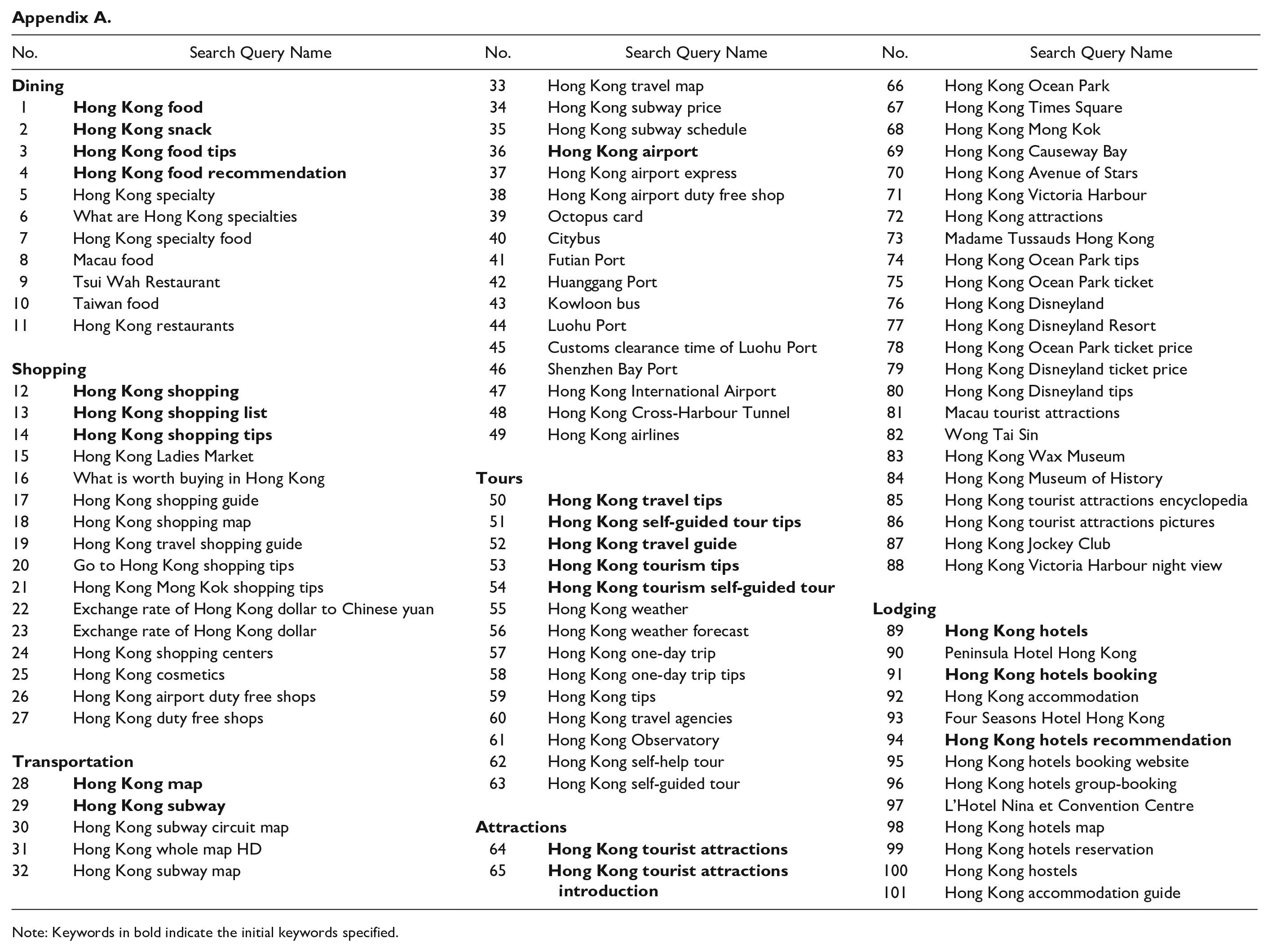
Ultimately, 101 Baidu search queries were collected (the names of the translated search queries can be found in Appendix A).

With this large number of search queries, some AI models, such as the deep learning models used in Law et al. (2019), can directly incorporate these search queries and identify the most relevant ones. However, most econometric models, including the MIDAS models used in this study, cannot perform this task. As a result, the dimensionality of the search queries must be reduced before the modeling process. This can be done by extracting common components using various factor models, such as static and dynamic factor models. Static factor models express common components as a linear combination of a small number of unobserved static factors that are loaded simultaneously (Stock and Watson 2002). The GDFM proposed by Forni et al. (2000) encompasses the static factor model, and its common components, $χ_{i t}$ , are driven by $q$ unobservable common factors, $f_{j t}$ , $j = 1, \dots, q$ . For the observed variables ${X_{i t}, i = 1, \dots, n, t = 1, \dots, T}$ , the model can be formulated as

X_{i t} = χ_{i t} + ε_{i t},

(1)

χ_{i t} = b_{i 1} (L) f_{1 t} + b_{i 2} (L) f_{2 t} + \dots + b_{i q} (L) f_{q t},

(2)

where $b_{i j} (L) = \sum_{k = 1}^{\infty} b_{i j k} L^{k}$ is the factor loading, $L$ is the lag operator, and $ε_{i t}$ is the idiosyncratic component. The GDFM has two important characteristics: it is dynamic and allows for cross-correlation among idiosyncratic components. Unlike static factor models, in which lagged factors are added as additional static factors, the common components of the GDFM can accommodate AR and MA responses. Distinguishing between leading and coincident variables a priori is not needed. The common components of the GDFM depend on cross-correlations at all leads and lags, so they can incorporate different lead and lag information from the variables (Forni et al. 2000). This is advantageous for constructing a composite index from a large number of search queries.

The GDFM has been adopted by several economic and financial institutions to analyze and predict economic activities. The Banca d’Italia published a real-time monthly coincident indicator of the euro area business cycle (Eurocoin) based on the GDFM (Altissimo et al. 2010). The Federal Reserve Bank of New York developed a similar index for estimating underlying inflation using these methods (Amstad and Potter 2009). In the tourism context, X. Li et al. (2017) were the first to use the GDFM to construct the composite index from Baidu search queries. They found that the GDFM-based index had better forecasting performance than principal components analysis. Therefore, the GDFM was adopted in this study to construct the index.

Before estimating the GDFM, a number of common factors, $q$ , must be determined. To this end, Forni et al. (2000) used the variance contribution rate, where $q$ is the number of factors whose variance contribution rates converge. However, this is a heuristic eye inspection rule. Nevertheless, Hallin and Liška (2007) proposed a formal test, using the log criterion of their study with the penalty function $p_{1}$ and lag window $\sqrt{T}$ to choose the number of factors, the maximum number of factors being set to 50. $c$ is the coefficient associated with the penalty function, $S_{c}$ is defined as the variability of the estimated $q$ when the size of the subsample increases, and $q_{c; n}^{* T}$ is the estimated $q$ when the whole sample is used. The selection of $q$ can be based on the plot of $S_{c}$ and $q_{c; n}^{* T}$ on $c$ , where $c$ is based on the second stability interval (more details are provided by Hallin and Liška 2007). This method was applied to the search queries of this study. The plot is shown in Figure 1.

Figure 1.

Log criterion for factor selection.

The second stability interval appeared at the interval between 0.31 and 0.34 (with $S_{c}$ equal to 0) and the estimated $q$ was equal to 4. Therefore, the number of common factors was set to 4 for the search queries.

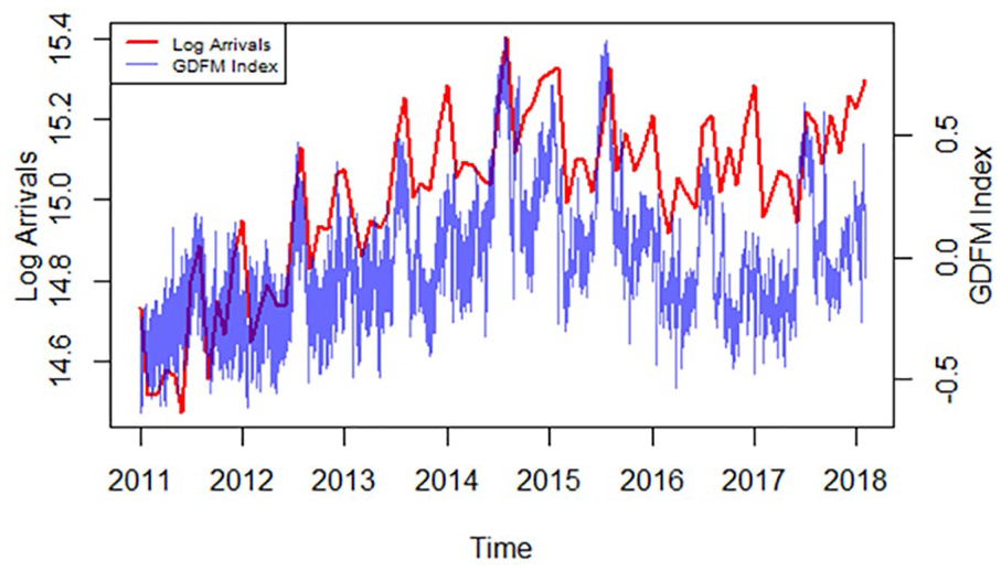
The common components were then calculated using standardized search query data with a mean of 0 and a standard deviation of 1. The coincidental index at time t was constructed using the common components, $z_{t} = \sum_{i = 1}^{n} χ_{i t}$ . As the search queries were collected daily, this index also had a daily frequency. The relationship between the daily index and the log transformation of monthly tourist arrivals is plotted in Figure 2.

Figure 2.

Daily index and log of tourist arrivals.

The close relationship between the daily index and monthly tourist arrivals is clearly illustrated.

Research Methods

In this section, the specifications and estimation procedure of the following competing models are presented: the SARIMA model, the SARIMA model with an exogenous variable (SARIMAX), and the traditional and improved MIDAS models. Data up to February 2017 were used for the estimation procedure, and the remaining data were used to evaluate the forecasting performance.

SARIMA and SARIMAX

The SARIMA model can account for seasonality, which is a common feature of tourism demand. It is the most commonly used time series model in the tourism demand forecasting literature and is often used as a benchmark (Song and Li 2008; D. C. Wu, Song, and Shen 2017). A SARIMA (p, d, q)(P, D, Q) model with seasonal frequency m can be specified as follows:

Φ (B^{m}) ϕ (B) {(1 - B^{m})}^{D} {(1 - B)}^{d} y_{t} = c + Θ (B^{m}) θ (B) ϵ_{t},

(3)

where $y_{t}$ is the log of tourist arrivals, $B$ is the backshift operator, $Φ (x)$ and $Θ (x)$ represent the seasonal AR and MA components (which are polynomials of order P and Q), respectively, $ϕ (x)$ and $θ (x)$ represent the nonseasonal AR and MA components (which are polynomials of order p and q), respectively, and $ϵ_{t}$ is a white noise process. The forecast package in the R 3.3.0 program (R Core Team 2016) was used to automatically select the orders and estimate the coefficients (Hyndman and Khandakar 2008) as follows:

The order of seasonal differencing $D$ was chosen using a test suggested by Wang, Smith, and Hyndman (2006), which is based on a measure of seasonal strength.

The order of nonseasonal differencing $d$ was chosen using the KPSS unit-root test (Kwiatkowski et al. 1992).

A stepwise procedure was used to traverse the model space and the orders and p, q, P, and Q were chosen based on the corrected Akaike information criterion (AIC).

The SARIMAX model simply adds an exogenous variable to SARIMA so that it becomes a regression model with SARIMA errors. Therefore, the estimation procedure of the SARIMAX model is almost identical to that of the SARIMA model, except that the regression is conducted first. It can be formulated as follows:

y_{t} = β_{0} + β_{1} x_{t} + n_{t}

(4)

Φ (B^{m}) ϕ (B) {(1 - B^{m})}^{D} {(1 - B)}^{d} n_{t} = Θ (B^{m}) θ (B) ϵ_{t},

(5)

where $x_{t}$ is the exogenous variable (which may include lagged variables) and $n_{t}$ is the error from the regression model. It is equivalent to substituting the differencing terms in the following regression equation:

{(1 - B^{m})}^{D} {(1 - B)}^{d} y_{t} = {(1 - B^{m})}^{D} {(1 - B)}^{d} (β_{0} + β_{1} x_{t}) + {n^{'}}_{t}

(6)

Φ (B^{m}) ϕ (B) {n^{'}}_{t} = Θ (B^{m}) θ (B) ϵ_{t},

(7)

where ${n^{'}}_{t}$ is ${(1 - B^{m})}^{D} {(1 - B)}^{d} n_{t}$ . Furthermore, this is equivalent to differencing $y_{t}$ and $x_{t}$ before fitting the model with ARMA errors. As nonstationary errors suggest the existence of spurious regression, it is necessary to difference the variables first.

The SRIMAX model can be rewritten as follows:

\begin{array}{l} {(1 - B^{m})}^{D} {(1 - B)}^{d} Φ (B^{m}) ϕ (B) y_{t} = {(1 - B^{m})}^{D} \\ {(1 - B)}^{d} Φ (B^{m}) ϕ (B) (β_{0} + β_{1} x_{t}) + Θ (B^{m}) θ (B) ϵ_{t} . \end{array}

(8)

It can be seen that the same AR terms are applied to $y_{t}$ and $x_{t}$ .

The exogenous variable used in this study was the composite index constructed from the search queries using the GDFM. As it was available daily, temporal aggregation was conducted by averaging the daily index for each month. However, the number of days varies in different months. To enable a direct comparison between the SARIMAX and MIDAS models, the 30 days preceding the first day of each month were considered to be a full last month. The monthly composite index at time t is denoted as $i n d e x_{t}$ .

The monthly index with at least one lag was added to the SARIMAX model, and the lag length was determined based on the AIC and the Bayesian information criterion (BIC). A monthly index with one lag was found to generate the smallest AIC and BIC.

After estimation, the fitted SARIMA and SARIMAX models can be written as

\begin{array}{l} S A R I M A : (1 + 0.2651 B - 0.5819 B^{2}) (1 - B^{12}) (1 - B) y_{t} \\ = (1 - 0.6750 B^{12}) (1 - 1.0745 B + 1.2188 B^{2} - 0.4372 B^{3}) ϵ_{t}, \end{array}

(9)

S A R I M A X : {\begin{matrix} y_{t} = 0.2122 i n d e x_{t - 1} + n_{t} \\ \begin{array}{l} (1 - 0.8780 B - 0.5241 B^{2}) (1 - B^{12}) \\ (1 - B) n_{t} = (1 - 0.5468 B^{12}) ϵ_{t} \end{array} \end{matrix} .

(10)

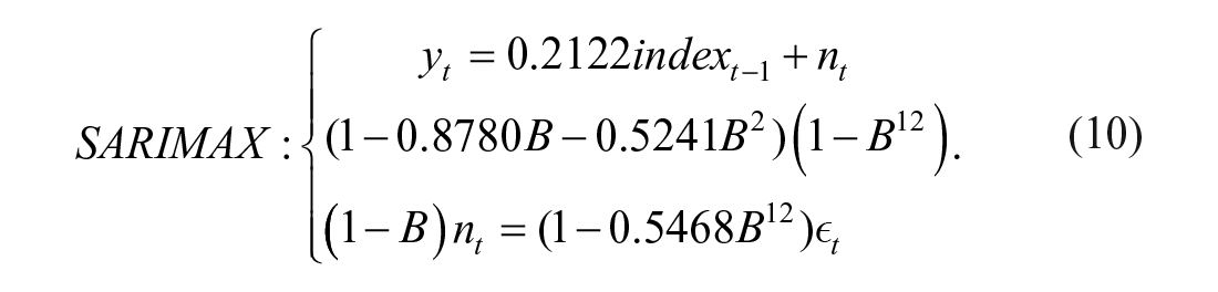
The details of the estimation results are summarized in Table 1.

Table 1.

Results of the SARIMA and SARIMAX Models.

SARIMA		SARIMAX
Nonseasonal differencing	Yes	Nonseasonal differencing	Yes
Seasonal differencing	Yes	Seasonal differencing	Yes
AR(1)	0.2651	AR(1)	−0.8780***
AR(2)	−0.5819***	AR(2)	−0.5241***
MA(1)	−1.0745***	SMA(1)	−0.5468***
MA(2)	1.2188***	$i n d e x_{t - 1}$	0.2122***
MA(3)	−0.4372**
SMA(1)	−0.6750***
Residual variance	0.00387	Residual variance	0.00356
AIC	−150.22	AIC	−157.74
BIC	−135.45	BIC	−147.27
Ljung-Box test	0.35	Ljung-Box test	0.70

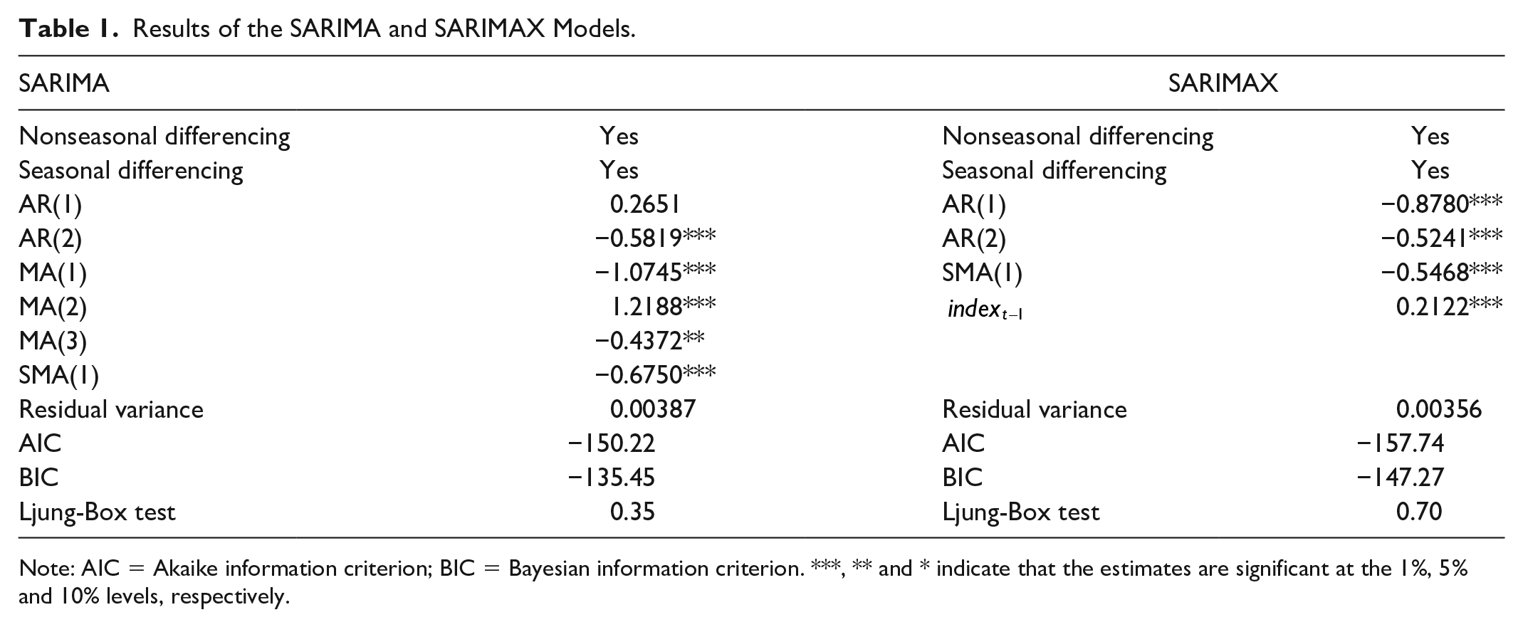
Note: AIC = Akaike information criterion; BIC = Bayesian information criterion. ***, ** and * indicate that the estimates are significant at the 1%, 5% and 10% levels, respectively.

The $i n d e x_{t - 1}$ coefficient was positive and significant at the 1% level, indicating that an increase in search queries leads to an increase in tourist arrivals the following month. The smaller AIC and BIC values of the SARIMAX model suggest that including the search query index fitted the model better. A Ljung-Box test was conducted to check the residuals of the fitted models and the p values were reported. The large p values indicate that the residuals were independently distributed and that the models were properly specified.

MIDAS Models

Search query data are available at a higher frequency than tourist arrival data. They contain potentially valuable information, and temporal aggregation can lead to information loss (Ghysels, Sinko, and Valkanov 2007). Most time series regressions involve data sampled at the same frequency, so high-frequency information cannot be used directly. As an alternative to the common solution of converting all data to the same low frequency, MIDAS can directly accommodate variables sampled at different frequencies. MIDAS models can be applied in cases where high-frequency variables are used to forecast a low-frequency variable. In addition, they may have more salient advantages when the frequencies of the variables are significantly different, as using traditional methods can lead to greater information loss during temporal aggregation. Therefore, MIDAS models are well suited to this study using monthly tourist arrivals and daily search queries.

The basic MIDAS model for a single explanatory variable can be written as

y_{t} = β_{0} + β_{1} \sum_{i = 1}^{l} ω (i; Θ) L_{H F}^{i} z_{t} + ϵ_{t},

(11)

where $y_{t}$ is the log of tourist arrivals, $L_{H F}$ is the high-frequency lag operator, $ω (i; Θ)$ is a polynomial that assigns the weights to the high-frequency variable $z_{t}$ at lag i, $l$ is the maximum lag on the high-frequency variable, and $ϵ_{t}$ is a white noise process.

Different weighting schemes can be used as functional constraints. A weighting scheme defined by the vector of parameters $Θ = (θ_{1}, θ_{2}, \dots, θ_{p})$ can be written as

ω (i; Θ) = \frac{f (i, Θ)}{\sum_{j = 1}^{l} f (j, Θ)} .

(12)

The most popular specifications for $f (i, Θ)$ include the exponential Almon function and the beta function (Ghysels, Sinko, and Valkanov 2007). Ghysels, Sinko, and Valkanov (2007) argued that the beta function was flexible enough to accommodate different weighting shapes with only two parameters. For comparison purposes, the exponential Almon specification used in this study also used two parameters. In addition, a Gompertz function was added as an additional comparison. The specifications of these three functions with two parameters ( $θ_{1}, θ_{2}$ ) are expressed below:

Exponential Almon: $f (i, Θ) = \exp (θ_{1} i + θ_{2} i^{2})$ .

Beta: $f (i, Θ) = \frac{{(k)}^{θ_{1} - 1} {(1 - k)}^{θ_{2} - 1} Γ (θ_{1} + θ_{2})}{Γ (θ_{1}) Γ (θ_{2})},$

where k = i/l, and Γ is the standard gamma function.

Gompertz: $f (i, Θ) = \exp (θ_{2} i) \exp (- θ_{1} \exp (θ_{2} i))$ .

MIDAS models can be expanded to include AR dynamics. However, this process is not straightforward, as noted by Ghysels, Sinko, and Valkanov (2007). Consider a MIDAS-AR model with one lag of $y_{t}$ :

y_{t} = β_{0} + λ y_{t - 1} + β_{1} \sum_{i = 1}^{l} ω (i; Θ) L_{H F}^{i} z_{t} + ϵ_{t} .

(13)

It can be rewritten as

y_{t} = β_{0} {(1 - λ)}^{- 1} + β_{1} {(1 - λ L_{L F})}^{- 1} \sum_{i = 1}^{l} ω (i; Θ) L_{H F}^{i} z_{t} + \tilde{{\tilde{ϵ}}_{t}},

(14)

where $L_{L F}$ is the low-frequency lag operator and $\tilde{{\tilde{ϵ}}_{t}} = {(1 - λ L_{L F})}^{- 1} ϵ_{t}$ . The polynomial on $z_{t}$ is a combination of $L_{L F}$ and $L_{H F}$ . This generates a seasonal response of $y_{t}$ to $z_{t}$ , whether $z_{t}$ demonstrates seasonal patterns. This strategy is generally considered inappropriate. Therefore, Clements and Galvão (2008) suggested introducing AR dynamics in $y_{t}$ as a common factor,

y_{t} = β_{0} + λ y_{t - 1} + β_{1} \sum_{i = 1}^{l} ω (i; Θ) L_{H F}^{i} (1 - λ L_{L F}) z_{t} + ϵ_{t},

(15)

where the same AR dynamics are applied to $y_{t}$ and $z_{t}$ so that the response of $y_{t}$ to $z_{t}$ is nonseasonal. This model was adopted in this study as MIDAS-AR. Before estimating MIDAS-AR, the amount of seasonal and nonseasonal differencing for tourist arrivals was determined using the same tests as the SARIMA model (Kwiatkowski et al. 1992; Wang, Smith, and Hyndman 2006). The same orders of differencing were applied to the daily index for interpretability. In addition, the AR orders were chosen based on the AIC and BIC.

MIDAS-AR models are less effective when MA dynamics are involved; therefore, it is desirable to include MA components in MIDAS. Foroni, Marcellino, and Stevanovic (2019) proved the usefulness of incorporating MA components into MIDAS models to predict US macroeconomic variables. However, they did not consider seasonal components, and the orders of ARMA components were determined arbitrarily. To remedy these shortcomings, an improved MIDAS model integrating MIDAS and SARIMA (MIDAS-SARIMA) was proposed. This model can be written as

y_{t} = β_{0} + β_{1} \sum_{i = 1}^{l} ω (i; Θ) L_{H F}^{i} z_{t} + n_{t} .

(16)

The difference between this new model and a standard MIDAS is that $n_{t}$ is a SARIMA process. Thus, the MIDAS-SARIMA model can accommodate seasonal and nonseasonal ARMA dynamics. This model is distinguished from standard MIDAS models by its seasonal structure. In addition, it integrates the automatic order selection procedure of SARIMA models to determine the best structure of the MIDAS-SARIMA model. As a result, this model combines the advantages of the MIDAS and SARIMA models and offers considerable potential to improve forecasting accuracy.

The MIDAS-SARIMA model applies the same AR dynamics to $y_{t}$ and $z_{t}$ . The estimation procedure of the MIDAS-SARIMA model is the same as that of the SARIMAX model, except that the first step is a MIDAS regression instead of a linear regression.

Unlike the SARIMAX model, which assigns the same weights to the high-frequency variable after temporal aggregation, the MIDAS-SARIMA model relaxes this restriction, which is useful because the search query data for different days are likely to have different effects on monthly tourist arrivals. This may lead to different weights of the daily composite index. The flexibility provided by the MIDAS-SARIMA model probably improves the forecasting accuracy of monthly tourist arrivals.

The number of lags of the daily composite index was set to 30 for MIDAS models in accordance with the SARIMAX model. That is, the 30 daily indices preceding the first day of the month were used to forecast tourist arrivals for the following month. This setting enabled a direct comparison between the SARIMAX and MIDAS models. The estimation results of the MIDAS-AR and MIDAS-SARIMA models are summarized in Table 2. MIDAS-AR-Almon, MIDAS-AR-Beta, and MIDAS-AR-Gom denote MIDAS-AR models with the exponential Almon, beta, and Gompertz weighting schemes, respectively. MIDAS-SARIMA-Almon, MIDAS-SARIMA-Beta, and MIDAS-SARIMA-Gom denote MIDAS-SARIMA models with the exponential Almon, beta, and Gompertz weighting schemes, respectively.

Table 2.

Results of the MIDAS-AR and MIDAS-SARIMA Models.

MIDAS-AR-Almon		MIDAS-AR-Beta		MIDAS-AR-Gom		MIDAS-SARIMA-Almon		MIDAS-SARIMA-Beta		MIDAS-SARIMA-Gom
Nonseasonal differencing	Yes	Nonseasonal differencing	Yes	Nonseasonal differencing	Yes	Nonseasonal differencing	Yes	Nonseasonal differencing	Yes	Nonseasonal differencing	Yes
Seasonal differencing	Yes	Seasonal differencing	Yes	Seasonal differencing	Yes	Seasonal differencing	Yes	Seasonal differencing	Yes	Seasonal differencing	Yes
$β_{1}$	0.2342**	$β_{1}$	0.2349**	$β_{1}$	0.2376**	$β_{1}$	0.2932**	$β_{1}$	0.2788**	$β_{1}$	0.2881**
$θ_{1}$	−0.1196	$θ_{1}$	0.9607***	$θ_{1}$	1.9965	$θ_{1}$	0.2809	$θ_{1}$	1.1262	$θ_{1}$	0.7226
$θ_{2}$	0.0026	$θ_{2}$	1.0779	$θ_{2}$	0.5920	$θ_{2}$	−0.0281	$θ_{2}$	8.1216	$θ_{2}$	3.9867
AR(1)	−0.9096***	AR(1)	−0.9274***	AR(1)	−0.9141***	MA(1)	−0.6464***	MA(1)	−0.6559***	MA(1)	−0.6465***
AR(2)	−0.5265***	AR(2)	−0.5348***	AR(2)	−0.5353***	SMA(1)	−0.5540***	SMA(1)	−0.5077***	SMA(1)	−0.5437***
AIC	−139.10	AIC	−138.91	AIC	−138.65	AIC	−145.96	AIC	−145.86	AIC	−146.21
BIC	−128.80	BIC	−128.60	BIC	−128.35	BIC	−133.39	BIC	−133.30	BIC	−133.64
Ljung- Box test	0.29	Ljung- Box test	0.31	Ljung- Box test	0.27	Ljung- Box test	0.38	Ljung- Box test	0.53	Ljung- Box test	0.48

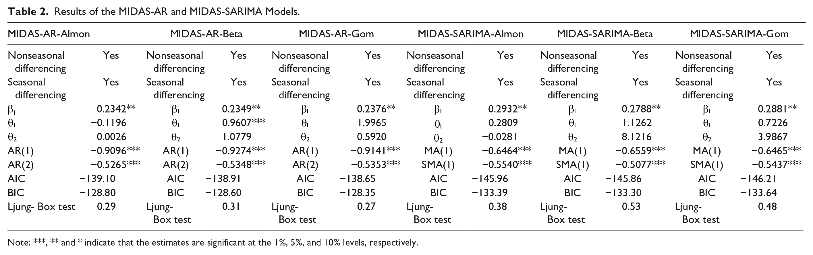
Note: ***, ** and * indicate that the estimates are significant at the 1%, 5%, and 10% levels, respectively.

Seasonal and nonseasonal differencing were performed for all MIDAS models. The MIDAS-AR models gave the same structures, with two lags of the AR dynamics, and the estimated coefficients of the two AR components were close for different weighting schemes. The same was observed for the MIDAS-SARIMA models, which had the same MA(1) and SMA(1) structures and similar estimated coefficients. This suggests that the different weighting schemes made little difference in the estimation of the MIDAS models. This result is consistent with the results of Bangwayo-Skeete and Skeete (2015). The AIC and BIC values suggest that the MIDAS-SARIMA models had a better fit and were more appropriate than the MIDAS-AR models.

The weights of the daily indices can be visualized. For example, the weights of the 30 daily indices for the MIDAS-SARIMA models are plotted in Figure 3.

Figure 3.

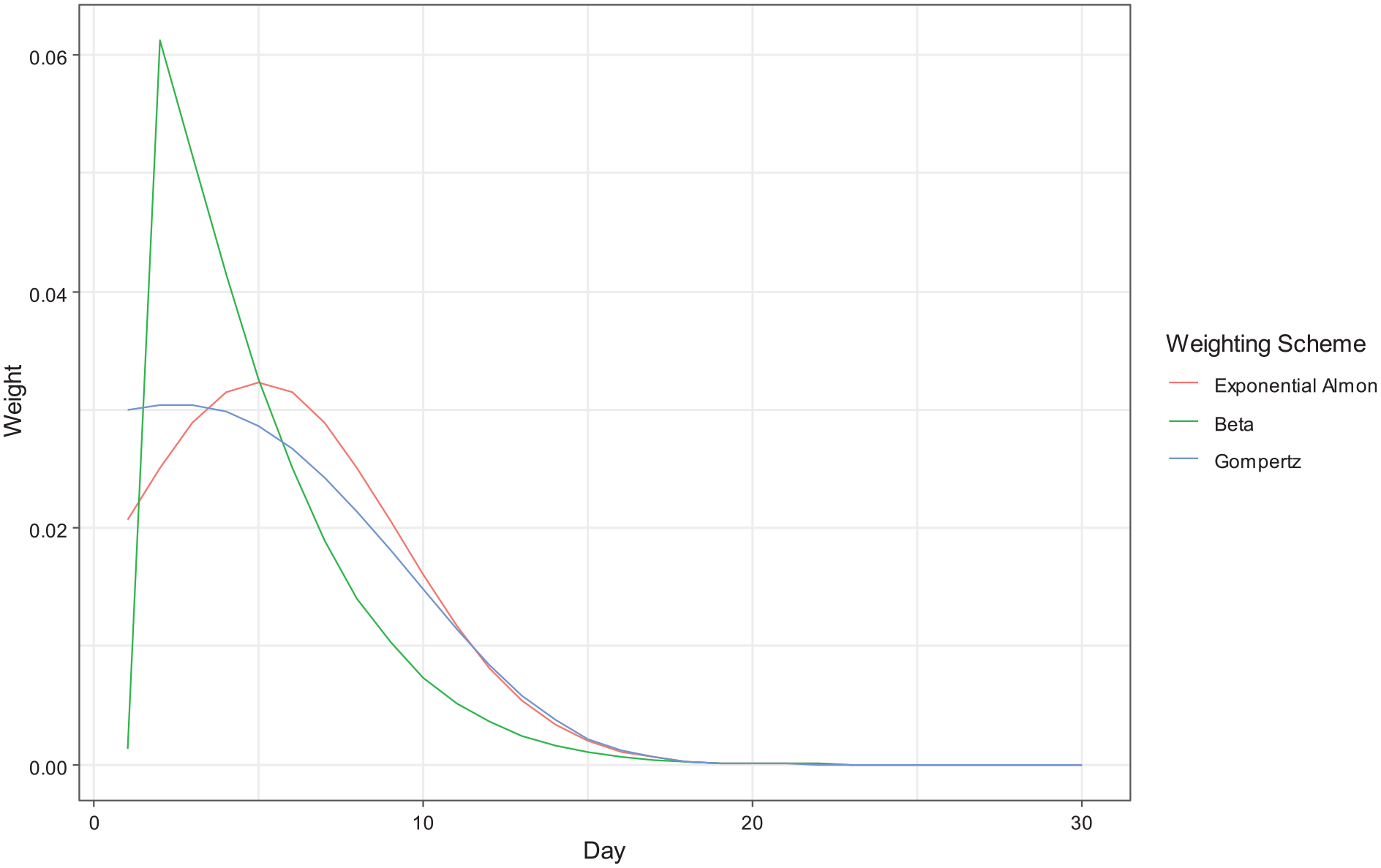
Different weighting schemes of the daily indices for the MIDAS-SARIMA models. The x-axis represents the number of days preceding the first day of the following month.

All three weighting schemes weighted the most recent indices more heavily. Most weights were put on the last 15 days, whereas the earlier days had almost 0 weight. Furthermore, the beta weighting scheme put the highest weight on day 2, whereas day 1 was given very little weight. The exponential Almon and Gompertz weighting schemes generated similar patterns to that of the beta weighting scheme. However, their weighting curves were much smoother than that of the beta weighting scheme. The close estimates of $β_{1}$ shown in Table 2 suggest that the total weights of the daily indices were similar.

Result Evaluation

Forecasting

In this subsection, the forecasting performance of the models using data from March 2017 to February 2018 is evaluated. Search query data with one lag were used in the modeling process, with the tourist arrivals and search query data available up to time t. Thus, the ARIMAX and MIDAS models had to first be estimated using tourist arrivals data up to time t and search query data up to time t–1. The results were then used to generate the forecasts at time t+1, with search query data at time t. Therefore, only one-step-ahead forecasts could be generated in this study. Longer-term forecasts may be further investigated in a future study with a different estimation procedure that uses search query data of lags longer than one but not conducted here. An expanding window approach was used to generate the one-step-ahead dynamic forecasts. For example, the data on tourist arrivals up to February 2017 and the search query data up to January 2017 were first used to estimate the models, then the search query data for February 2017 were used to forecast tourist arrivals in March 2017. The estimation period was then extended by 1 month, and the models were re-estimated using the same procedure. The forecasts were generated at each round until all 12 one-step-ahead forecasts were calculated for the period from March 2017 to February 2018.

Forecast accuracy was evaluated using five commonly used forecast error measures, including the mean absolute deviation (MAD), the mean squared error (MSE), the mean absolute percentage error (MAPE), the root mean square percentage error (RMSPE) and Theil’s U statistic (Goh and Law 2002; Law et al. 2019). The MAD and MSE are absolute error measures. In contrast, the MAPE and RMSPE are relative error measures. Finally, Theil’s U was constructed based on the error ratio of the underlying model to the seasonal naïve model. A seasonal naïve model basically predicts that monthly tourist arrivals for the following year will be the same as this year for the same month. A value less than 1 indicates that the performance of the model is superior to that of the naïve model. Their specifications are as follows:

MAD = \frac{1}{n} \sum_{t = 1}^{n} | A_{t} - F_{t} |

MSE = \frac{1}{n} \sum_{t = 1}^{n} {(A_{t} - F_{t})}^{2}

MAPE = \frac{1}{n} \sum_{t = 1}^{n} \frac{| A_{t} - F_{t} |}{A_{t}}

RMSPE = \sqrt{\frac{1}{n} \sum_{t = 1}^{n} {(\frac{A_{t} - F_{t}}{A_{t}})}^{2}}

U = \frac{\sqrt{\sum_{t = 1}^{n} {(A_{t} - F_{t})}^{2}}}{\sqrt{\sum_{t = 1}^{n} {(A_{t} - A_{t - 12})}^{2}}},

where $A_{t}$ is the actual value, $F_{t}$ is the forecast value at time t and n is the length of the forecast period (n = 12 in this study). Two extra benchmark models have been added to the forecasting practice: the ETS and the seasonal naïve model. Athanasopoulos et al. (2011) found that the ETS performed particularly well for monthly data in their tourism forecasting competition. The seasonal naïve model is also widely used as a benchmark model in forecasting seasonal tourism demand (Athanasopoulos et al. 2011). Table 3 presents the results of the models’ forecasting performance.

Table 3.

Evaluation of the One-Step-Ahead Dynamic Forecasts.

Measure	MAD	MSE	MAPE, %	RMSPE, %	Theil’s U
Seasonal Naïve	288,795	1.77E+11	7.30	10.01	1
ETS	286,297	1.24E+11	7.34	8.70	0.837
SARIMA	290,781	1.45E+11	7.46	9.33	0.904
SARIMAX	268,737	1.26E+11	6.94	8.83	0.844
MIDAS-AR-Almon	285,371	1.54E+11	7.31	9.63	0.932
MIDAS-AR-Beta	285,183	1.54E+11	7.30	9.62	0.933
MIDAS-AR-Gom	280,302	1.52E+11	7.19	9.58	0.927
MIDAS-SARIMA-Almon	248,653	1.08E+11	6.34	8.08	0.78
MIDAS-SARIMA-Beta	255,198	1.17E+11	6.58	8.52	0.814
MIDAS-SARIMA-Gom	250,081	1.06E+11	6.47	8.16	0.775

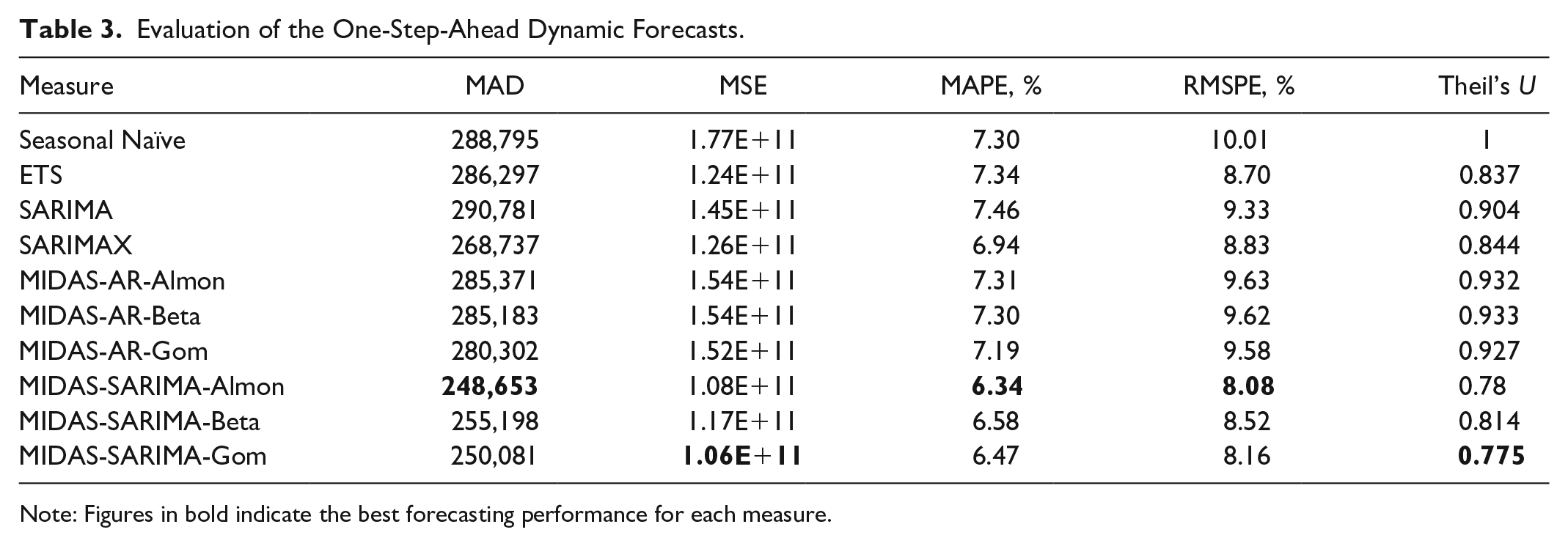
Note: Figures in bold indicate the best forecasting performance for each measure.

The rankings were mostly consistent based on the error measures. All of the models except for the seasonal naïve model had Theil’s U values of less than 1, suggesting that all of the models outperformed the seasonal naïve model in terms of the squared error (SE).

Overall, the seasonal naïve model performed the worst, especially in terms of the MSE and RMSPE. In contrast, the ETS performed well in terms of the MSE and RMSPE. The SARIMAX model performed better than the SARIMA model based on the error measures and showed that search queries improved the forecasting accuracy of tourist arrivals. This result is consistent with the findings of previous studies (X. Li et al. 2017; Pan, Wu, and Song 2012; Pan and Yang 2017; Yang et al. 2015). The MIDAS-AR models generated forecasts comparable to those of SARIMA and only outperformed SARIMA in terms of the MAPE and MAD. This result contrasts the findings of Bangwayo-Skeete and Skeete (2015). The MIDAS-AR models were also outperformed by the SARIMAX and MIDAS-SARIMA models, indicating that traditional MIDAS models have limitations when using the information provided by high-frequency search query data. The SARIMAX model performed well because of its flexibility to incorporate seasonal and nonseasonal ARMA components. Finally, the MIDAS-SARIMA models demonstrated the best performance in terms of all measures and remarkable improvements compared with the MIDAS-AR models. Thus, this improved MIDAS model combining the strengths of the MIDAS and SARIMAX models improved the forecasting performance. The results also suggest that forecasting performance was improved by integrating MA components into MIDAS models, which is consistent with the findings of Foroni, Marcellino, and Stevanovic (2019).

MIDAS-SARIMA-Almon demonstrated the best performance based on the MAD, MAPE, and RMSPE, whereas MIDAS-SARIMA-Gom demonstrated the best performance based on the MSE and Theil’s U. Overall, different weighting schemes generated comparable forecasting performance, which is consistent with the findings of Bangwayo-Skeete and Skeete (2015). The results also indicate that the most recent search query data, which were assigned most weights in the MIDAS-SARIMA models, were the most valuable in predicting tourist arrivals.

To further test the significance of forecasting differences between the two better benchmark models (SARIMA and ETS) and the models using search query data, a Diebold-Mariano (DM) test was conducted (Diebold and Mariano 1995). The test was based on the forecasting differences of four measures, namely, the absolute deviation, the SE, the absolute percentage error (APE), and the squared percentage error (SPE), which were used to calculate the MAD, MSE, MAPE, and RMSPE, respectively. As Theil’s U had the same denominator derived from the seasonal naïve model and its numerator was calculated from the MSE; the corresponding DM test largely depended on the MSE and was therefore omitted. Tables 4 and 5 present the results of the DM tests for SARIMA and the ETS, respectively. The null hypothesis of the DM test is that the accuracy of the forecasts generated by the benchmark and alternative models does not differ.

Table 4.

DM Test Statistics for SARIMA.

Measure	AE	SE	APE	SPE
SARIMAX	−0.935	−1.083	−0.804	−0.818
MIDAS-AR-Almon	−0.179	0.370	−0.182	0.359
MIDAS-AR-Beta	−0.186	0.384	−0.201	0.358
MIDAS-AR-Gom	−0.334	0.296	−0.317	0.301
MIDAS-SARIMA-Almon	−2.107**	−1.484*	−2.260**	−1.669**
MIDAS-SARIMA-Beta	−2.101**	−1.431*	−1.902**	−1.334*
MIDAS-SARIMA-Gom	−2.081**	−1.328*	−2.084**	−1.338*

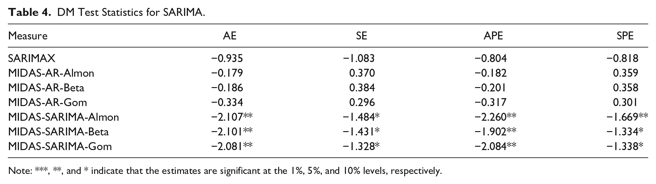
Note: ***, **, and * indicate that the estimates are significant at the 1%, 5%, and 10% levels, respectively.

Table 5.

DM Test Statistics for ETS.

Measure	AE	SE	APE	SPE
SARIMAX	−0.757	0.189	−0.629	0.271
MIDAS-AR-Almon	−0.023	0.712	−0.025	0.693
MIDAS-AR-Beta	−0.029	0.719	−0.041	0.695
MIDAS-AR-Gom	−0.148	0.669	−0.138	0.655
MIDAS-SARIMA-Almon	−2.213**	−1.578*	−2.209**	−1.656**
MIDAS-SARIMA-Beta	−1.323	−0.510	−1.193	−0.325
MIDAS-SARIMA-Gom	−1.812**	−1.219	−1.628*	−1.012

Note: ***, **, and * indicate that the estimates are significant at the 1%, 5%, and 10% levels, respectively.

As indicated by the DM test statistics, although the SARIMAX model outperformed the SARIMA model, the difference was not significant. Only the MIDAS-SARIMA models performed significantly better than SARIMA based on the error measures (at least at the 10% significance level), confirming the superiority of the proposed model and highlighting the importance of added flexibility to accommodate MA dynamics in MIDAS models. In the case of the ETS, only MIDAS-SARIMA-Almon generated significantly better results in terms of all measures. MIDAS-SARIMA-Gom significantly outperformed the ETS in terms of the AE and APE.

Nowcasting

The traditional models used in this study, such as the benchmark models and ARIMAX, are unable to update the forecasts until a full month of search query data are available, as they cannot incorporate high-frequency search query data that offer a new daily index after each day. However, daily nowcasts can be generated using MIDAS models as new search query data become available every day. For example, when the search query data for the first day of the month are available, they can be added to the MIDAS models and used to predict tourist arrivals for that month (nowcasting). This can be repeated every day until the end of the month. Again, because of the variable number of days in each month, nowcasts with search query data for 30 days starting from the first day of the same month were produced. As the MIDAS-SARIMA models had the best forecasting performance, their nowcasting performance was further investigated. Nowcasting is conducted in a similar way to forecasting. Nowcasting models must be refitted when new daily search query data become available, using the monthly tourist arrivals data until the end of the last month and the daily search query data until the end of that day. Then the nowcasts of the monthly tourist arrivals in the current month can be generated. This process can be repeated over an entire month to update the nowcasts of tourist arrivals in that month. The accuracy of these nowcasts can be investigated to determine whether updated nowcasts with more daily search query data perform better.

Nowcasting performance is plotted against the number of days of search query data added in Figures 4 –8. The X axis represents the number of days of search query data added to generate the nowcasts. Day 0 denotes the forecasting performance of the same model. The horizontal dotted line drawn on the forecasting performance level facilitates the comparison between forecasts and nowcasts.

Figure 4.

MAD of Nowcasting for the MIDAS-SARIMA Models with Different Weighting Schemes.

Figure 5.

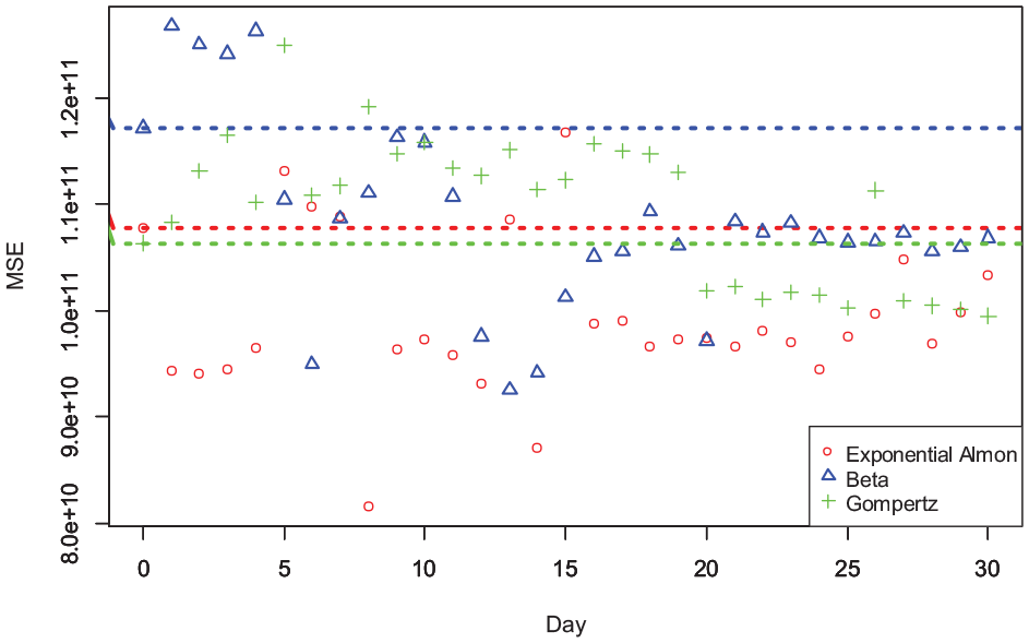
MSE of nowcasting for the MIDAS-SARIMA models with different weighting schemes.

Figure 6.

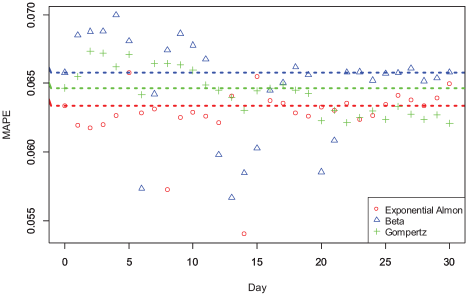
MAPE of nowcasting for the MIDAS-SARIMA models with different weighting schemes.

Figure 7.

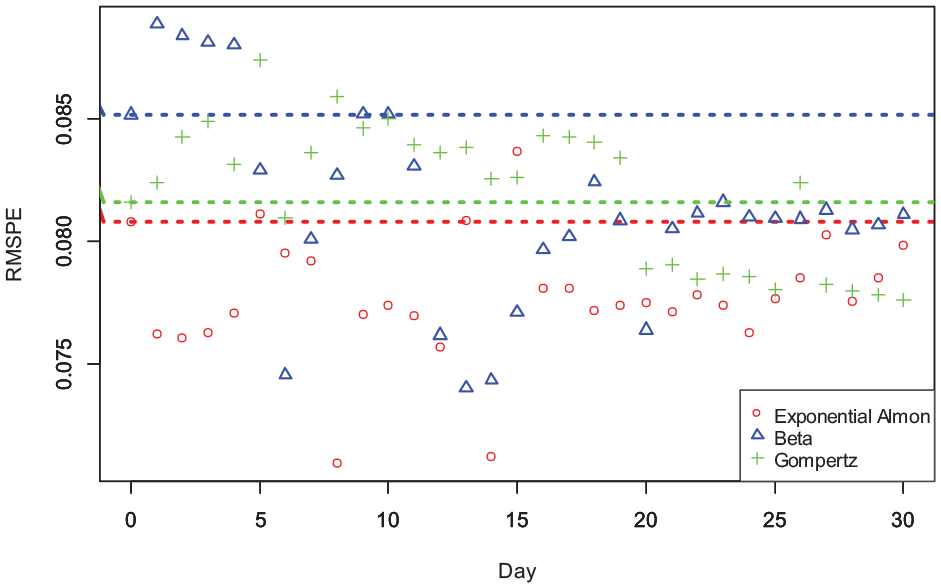
RMSPE of nowcasting for the MIDAS-SARIMA models with different weighting schemes.

Figure 8.

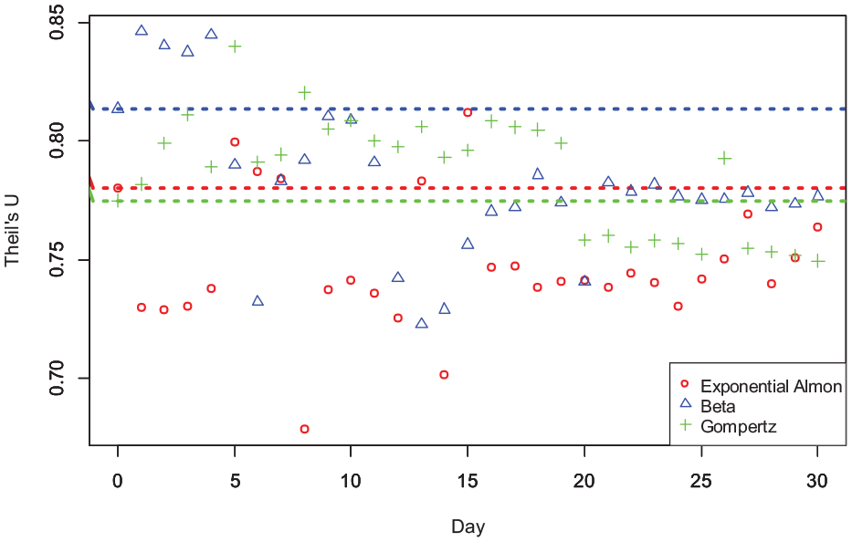
Theil’s U of nowcasting for the MIDAS-SARIMA models with different weighting schemes.

The nowcasts showed a certain level of fluctuation for all models. Overall, the exponential Almon weighting scheme gave the best results. In addition, most of the points were below the dotted forecasting line of the corresponding color, which became more apparent as the number of days increased. This suggests that nowcasting generally outperforms forecasting using the MIDAS-SARIMA models, especially when more data become available. The percentage of the nowcasts outperforming the forecasts were calculated for each model, as shown in Table 6. The exponential Almon and beta weighting schemes had more nowcasts that outperformed the forecasts based on all measures. However, the Gompertz weighting scheme had better nowcasts only with respect to the MAPE. Nevertheless, a downward trend was still visible for the Gompertz weighting scheme (as shown in Figures 4 –8), indicating that the nowcasts generally improved as more search query data became available.

Table 6.

Percentage of Nowcasts Outperforming Forecasts.

Measure	MAD	MSE	MAPE	RMSPE	Theil’s U
MIDAS-SARIMA-Almon	0.73	0.83	0.60	0.90	0.83
MIDAS-SARIMA-Beta	0.63	0.87	0.53	0.80	0.87
MIDAS-SARIMA-Gom	0.50	0.33	0.63	0.37	0.33

Conclusion

Search query data are increasingly used to improve the accuracy of tourism demand forecasting. The aim of this study was to investigate the performance of an improved MIDAS model (the MIDAS-SARIMA model) with the flexibility to accommodate seasonal and nonseasonal ARMA dynamics in predicting monthly tourist arrivals in Hong Kong from mainland China. The results confirmed the superiority of the proposed MIDAS-SARIMA model compared with traditional MIDAS and other benchmark models.

Traditional MIDAS-AR models are ineffective when MA dynamics are involved. The MIDAS-AR models produced similar results to those of the benchmark model and were outperformed by the SARIMAX model. Although MIDAS-AR could better use the valuable information contained in the high frequency data, this advantage was outweighed by the limitation of its structure. The improved forecasting performance of the proposed MIDAS-SARIMA model compared with the MIDAS-AR models is consistent with the findings of Foroni, Marcellino, and Stevanovic (2019), who demonstrated the relevance of MA components in MIDAS models in forecasting macroeconomic variables. In addition to accommodating MA components, the MIDAS-SARIMA model proposed in this study could incorporate seasonal ARMA components and automatically choose appropriate structures. As a result, the MIDAS-SARIMA model produced the best forecasts and was the only model that could significantly outperform the SARIMA benchmark model, as indicated by the DM tests.

A comparison of forecasts and nowcasts was also conducted. As new search query data became available, their information could be incorporated into the MIDAS models using the mixed frequency structure and daily nowcasts could be generated. The nowcasts outperformed the forecasts most of the time for the exponential Almon and beta weighting schemes. Although the forecasts of the Gompertz weighting scheme outperformed most nowcasts, the scheme overall showed a downward trend in error measures. Thus, the nowcasts were generally more accurate as more search query data became available.

The results of this study have important implications for research in this area. Search query data have received considerable attention in forecasting tourism demand in recent years. However, using the valuable information contained in these data is problematic and requires appropriate methods. Bangwayo-Skeete and Skeete (2015) were the first to use MIDAS models, which were found to have better forecasting performance than benchmark time series models. However, they did not compare these MIDAS models with models that could also include search query information, such as the SARIMAX model. Therefore, whether the benefits of MIDAS can outweigh the cost of the limitations of its structure is unclear. Indeed, some studies have found no evidence supporting the use of mixed frequency methods (Rivera 2016). The forecasting performance of MIDAS models is likely to be hindered by their inability to accommodate MA dynamics. The improved MIDAS model proposed in this study not only overcame this shortcoming but also accommodated seasonal dynamics. In addition, the automatic structure determination reduced the risk of misspecification. Overall, the forecasting results confirm the merits of this new model.

The results of this study also have implications for decision makers in the tourism sector. Specifically, they confirm the value of search query data in forecasting tourism demand, showing that forecasting accuracy can be further improved using the improved MIDAS model. The benefits of this improved forecasting accuracy are significant, as indicated by the DM tests, whereas the cost is minimal, as the search engine data can often be retrieved for free. Once the model is developed, updating the forecasts and nowcasts is easy. As nowcasts can be generated daily, they are particularly important for those who need frequent updates of tourism demand forecasts in their day-to-day business operations.

Various possibilities exist for future research. First, only search query data were used in this study. Other forms of big data, such as social media and device data, may be valuable predictors that can improve forecasting accuracy. In addition, the results suggest that the most recent search query data have more forecasting power. Therefore, improved forecasting accuracy may gradually disappear as the forecasting horizon increases. As only short-term forecasts were generated in this study, it would be interesting to see whether the usefulness of search query data wanes as the forecast horizon increases. Finally, more origin and destination pairs should be used to further generalize the results of this study.

Footnotes

Appendix

Appendix A.

No.	Search Query Name	No.	Search Query Name	No.	Search Query Name
Dining		33	Hong Kong travel map	66	Hong Kong Ocean Park
1	Hong Kong food	34	Hong Kong subway price	67	Hong Kong Times Square
2	Hong Kong snack	35	Hong Kong subway schedule	68	Hong Kong Mong Kok
3	Hong Kong food tips	36	Hong Kong airport	69	Hong Kong Causeway Bay
4	Hong Kong food recommendation	37	Hong Kong airport express	70	Hong Kong Avenue of Stars
5	Hong Kong specialty	38	Hong Kong airport duty free shop	71	Hong Kong Victoria Harbour
6	What are Hong Kong specialties	39	Octopus card	72	Hong Kong attractions
7	Hong Kong specialty food	40	Citybus	73	Madame Tussauds Hong Kong
8	Macau food	41	Futian Port	74	Hong Kong Ocean Park tips
9	Tsui Wah Restaurant	42	Huanggang Port	75	Hong Kong Ocean Park ticket
10	Taiwan food	43	Kowloon bus	76	Hong Kong Disneyland
11	Hong Kong restaurants	44	Luohu Port	77	Hong Kong Disneyland Resort
		45	Customs clearance time of Luohu Port	78	Hong Kong Ocean Park ticket price
Shopping		46	Shenzhen Bay Port	79	Hong Kong Disneyland ticket price
12	Hong Kong shopping	47	Hong Kong International Airport	80	Hong Kong Disneyland tips
13	Hong Kong shopping list	48	Hong Kong Cross-Harbour Tunnel	81	Macau tourist attractions
14	Hong Kong shopping tips	49	Hong Kong airlines	82	Wong Tai Sin
15	Hong Kong Ladies Market			83	Hong Kong Wax Museum
16	What is worth buying in Hong Kong	Tours		84	Hong Kong Museum of History
17	Hong Kong shopping guide	50	Hong Kong travel tips	85	Hong Kong tourist attractions encyclopedia
18	Hong Kong shopping map	51	Hong Kong self-guided tour tips	86	Hong Kong tourist attractions pictures
19	Hong Kong travel shopping guide	52	Hong Kong travel guide	87	Hong Kong Jockey Club
20	Go to Hong Kong shopping tips	53	Hong Kong tourism tips	88	Hong Kong Victoria Harbour night view
21	Hong Kong Mong Kok shopping tips	54	Hong Kong tourism self-guided tour
22	Exchange rate of Hong Kong dollar to Chinese yuan	55	Hong Kong weather	Lodging
23	Exchange rate of Hong Kong dollar	56	Hong Kong weather forecast	89	Hong Kong hotels
24	Hong Kong shopping centers	57	Hong Kong one-day trip	90	Peninsula Hotel Hong Kong
25	Hong Kong cosmetics	58	Hong Kong one-day trip tips	91	Hong Kong hotels booking
26	Hong Kong airport duty free shops	59	Hong Kong tips	92	Hong Kong accommodation
27	Hong Kong duty free shops	60	Hong Kong travel agencies	93	Four Seasons Hotel Hong Kong
		61	Hong Kong Observatory	94	Hong Kong hotels recommendation
Transportation		62	Hong Kong self-help tour	95	Hong Kong hotels booking website
28	Hong Kong map	63	Hong Kong self-guided tour	96	Hong Kong hotels group-booking
29	Hong Kong subway			97	L’Hotel Nina et Convention Centre
30	Hong Kong subway circuit map	Attractions		98	Hong Kong hotels map
31	Hong Kong whole map HD	64	Hong Kong tourist attractions	99	Hong Kong hotels reservation
32	Hong Kong subway map	65	Hong Kong tourist attractions introduction	100	Hong Kong hostels
32	Hong Kong subway map	65	Hong Kong tourist attractions introduction	101	Hong Kong accommodation guide

Note: Keywords in bold indicate the initial keywords specified.

Declaration of Conflicting Interests

The author(s) declared no potential conflicts of interest with respect to the research, authorship, and/or publication of this article.

Funding

The author(s) disclosed receipt of the following financial support for the research, authorship, and/or publication of this article: The Natural Science Foundation of China (NSFC) provided financial support for the study (Grant No. 71673233).

ORCID iDs

Long Wen

Haiyan Song

Han Liu

Author Biographies

Long Wen, PhD, is Assistant Professor in School of Economics at University of Nottingham Ningbo China. His research interests are mainly in tourism economics, tourism demand modeling and forecasting.

Chang Liu, PhD, is Professor and deputy head of School of Economics at University of Nottingham Ningbo China. His research interests include international trade, foreign direct investment and regional economics.

Haiyan Song, PhD, is Mr and Mrs Chan Chak Fu Professor in International Tourism in the School of Hotel and Tourism at The Hong Kong Polytechnic University. His research interests include tourism demand modeling and forecasting, tourism supply chain management and wine economics.

Han Liu, PhD, is Assistant Professor in the Center for Quantitative Economics and Business School at Jilin University. His research interests are in the areas of applied econometrics related to tourism demand modeling and forecasting.

References

Aladag

C. H.

Egrioglu

Yolcu

Uslu

V. R.

2014. “A High Order Seasonal Fuzzy Time Series Model and Application to International Tourism Demand of Turkey.” Journal of Intelligent and Fuzzy Systems 26 (1): 295–302.

Altissimo

Cristadoro

Forni

Lippi

Veronese

2010. “New Eurocoin: Tracking Economic Growth in Real Time.” Review of Economics and Statistics 92 (4): 1024–34.

Amstad

Potter

2009. “Real Time Underlying Inflation Gauges for Monetary Policymakers.” FRB of New York Staff Report, 420.

Andreou

Ghysels

Kourtellos

2013. “Should Macroeconomic Forecasters Use Daily Financial Data and How?” Journal of Business & Economic Statistics 31 (2): 240–51.

Askitas

Zimmermann

K. F.

2009. “Google Econometrics and Unemployment Forecasting.” Applied Economics Quarterly 55 (2): 107–20.

Assaf

A. G.

Barros

C. P.

Gil-Alana

L. A.

2011. “Persistence in the Short- and Long-Term Tourist Arrivals to Australia.” Journal of Travel Research 50 (2): 213–29.

Athanasopoulos

Hyndman

R. J.

Song

D. C.

2011. “The Tourism Forecasting Competition.” International Journal of Forecasting 27 (3): 822–44.

Bangwayo-Skeete

P. F.

Skeete

R. W.

2015. “Can Google Data Improve the Forecasting Performance of Tourist Arrivals? Mixed-Data Sampling Approach.” Tourism Management 46:454–64.

Baumeister

Guérin

Kilian

2015. “Do High-Frequency Financial Data Help Forecast Oil Prices? The MIDAS Touch at Work.” International Journal of Forecasting 31 (2): 238–52.

10.

Bordino

Battiston

Caldarelli

Cristelli

Ukkonen

Weber

2012. “Web Search Queries Can Predict Stock Market Volumes.” PLoS One 7 (7): e40014.

11.

Brynjolfsson

Geva

Reichman

2014. “Using Crowd-Based Data Selection to Improve the Predictive Power of Search Trend Data.” The International Conference on Information Systems (ICIS 2014), Auckland, New Zealand.

12.

Chen

Liang

C. Y.

Hong

W. C.

D. X.

2015. “Forecasting Holiday Daily Tourist Flow Based on Seasonal Support Vector Regression with Adaptive Genetic Algorithm.” Applied Soft Computing 26:435–43.

13.

Choi

Varian

2012. “Predicting the Present with Google Trends.” Economic Record 88 (1): 2–9.

14.

Chu

F. L.

2009. “Forecasting Tourism Demand with ARMA-Based Methods.” Tourism Management 30 (5): 740–51.

15.

Claveria

Monte

Torra

2015. “Tourism Demand Forecasting with Neural Network Models: Different Ways of Treating Information.” International Journal of Tourism Research 17 (5): 492–500.

16.

Clements

M. P.

Galvão

A. B.

2008. “Macroeconomic Forecasting with Mixed-Frequency Data.” Journal of Business & Economic Statistics 26 (4): 546–54.

17.

Engelberg

Gao

2011. “In Search of Attention.” Journal of Finance 66 (5): 1461–99.

18.

Diebold

F. X.

Mariano

R. S.

1995. “Comparing Predictive Accuracy.” Journal of Business & Economic Statistics 13 (3): 253–63.

19.

Divino

J. A.

McAleer

2010. “Modelling and Forecasting Daily International Mass Tourism to Peru.” Tourism Management 31 (6): 846–54.

20.

R. Y.

Damangir

2014. “Leveraging Trends in Online Searches for Product Features in Market Response Modeling.” Journal of Marketing 79 (1): 29–43.

21.

R. Y.

Kamakura

W. A.

2012. “Quantitative Trendspotting.” Journal of Marketing Research 49 (4): 514–36.

22.

Fesenmaier

D. R.

Xiang

Pan

Law

2011. “A Framework of Search Engine Use for Travel Planning.” Journal of Travel Research 50 (6): 587–601.

23.

Forni

Hallin

Lippi

Reichlin

2000. “The Generalized Dynamic-Factor Model: Identification and Estimation.” Review of Economics and Statistics 82 (4): 540–54.

24.

Foroni

Marcellino

Stevanovic

2019. “Mixed-Frequency Models with Moving-Average Components.” Journal of Applied Econometrics 34 (5): 688–706.

25.

Ghose

Ipeirotis

P. G.

2014. “Examining the Impact of Ranking on Consumer Behavior and Search Engine Revenue.” Management Science 60 (7): 1632–54.

26.

Ghysels

Santa-Clara

Valkanov

2004. “The MIDAS Touch: Mixed Data Sampling Regression Models” (CIRANO Working Paper). CIRANO.

27.

Ghysels

Sinko

Valkanov

2007. “MIDAS Regressions: Further Results and New Directions.” Econometric Reviews 26 (1): 53–90.

28.

Ghysels

Valkanov

R. I.

Serrano

A. R.

2009. “Multi-Period Forecasts of Volatility: Direct, Iterated, and Mixed-Data Approaches.” In EFA 2009 Bergen Meetings Paper.

29.

Ginsberg

Mohebbi

M. H.

Patel

R. S.

Brammer

Smolinski

M. S.

Brilliant

2009. “Detecting Influenza Epidemics Using Search Engine Query Data.” Nature 457 (7232): 1012–14.

30.

Goh

2012. “Exploring Impact of Climate on Tourism Demand.” Annals of Tourism Research 39 (4): 1859–83.

31.

Goh

Law

2002. “Modeling and Forecasting Tourism Demand for Arrivals with Stochastic Nonstationary Seasonality and Intervention.” Tourism Management 23 (5): 499–510.

32.

Goh

Law

Mok

H. M.

2008. “Analyzing and Forecasting Tourism Demand: A Rough Sets Approach.” Journal of Travel Research 46 (3): 327–38.

33.

Gunter

Önder

2015. “Forecasting International City Tourism Demand for Paris: Accuracy of Uni- and Multivariate Models Employing Monthly Data.” Tourism Management 46:123–35.

34.

Gurgul

Mestel

Syrek

2018. “MIDAS Models in Banking Sector—Systemic Risk Comparison.” Managerial Economics 18 (2): 165–81.

35.

Hallin

Liška

2007. “Determining the Number of Factors in the General Dynamic Factor Model.” Journal of the American Statistical Association 102 (478): 603–17.

36.

Hassani

Silva

E. S.

Antonakakis

Filis

Gupta

2017. “Forecasting Accuracy Evaluation of Tourist Arrivals.” Annals of Tourism Research 63:112–27.

37.

Hassani

Webster

Silva

E. S.

Heravi

2015. “Forecasting U.S. Tourist Arrivals Using Optimal Singular Spectrum Analysis.” Tourism Management 46:322–35.

38.

Hong

W.-C.

Dong

Chen

L.-Y.

Wei

S.-Y.

2011. “SVR with Hybrid Chaotic Genetic Algorithms for Tourism Demand Forecasting.” Applied Soft Computing 11 (2): 1881–90.

39.

Hyndman

R. J.

Khandakar

2008. “Automatic Time Series Forecasting: The Forecast Package for R.” Journal of Statistical Software 27 (3): 1–22.

40.

Kambatla

Kollias

Kumar

Grama

2014. “Trends in Big Data Analytics.” Journal of Parallel and Distributed Computing 74 (7): 2561–73.

41.

Kwiatkowski

Phillips

P. C. B.

Schmidt

Shin

1992. “Testing the Null Hypothesis of Stationarity against the Alternative of a Unit Root.” Journal of Econometrics 54 (1): 159–78.

42.

Law

Fong

D. K. C.

Han

2019. “Tourism Demand Forecasting: A Deep Learning Approach.” Annals of Tourism Research 75:410–23.

43.

Song

Witt

S. F.

2006. “Time Varying Parameter and Fixed Parameter Linear AIDS: An Application to Tourism Demand Forecasting.” International Journal of Forecasting 22 (1): 57–71.

44.

Law

2020. “Forecasting Tourism Demand with Decomposed Search Cycles.” Journal of Travel Research 59 (1): 52–68.

45.

Pan

Law

Huang

2017. “Forecasting Tourism Demand with Composite Search Index.” Tourism Management 59:57–66.

46.

Monteforte

Moretti

2012. “Real-Time Forecasts of Inflation: The Role of Financial Variables.” Journal of Forecasting 32 (1): 51–61.

47.

Page

Song

D. C.

2012. “Assessing the Impacts of the Global Economic Crisis and Swine Flu on Inbound Tourism Demand in the United Kingdom.” Journal of Travel Research 51 (2): 142–53.

48.

Pan

D. C.

Song

2012. “Forecasting Hotel Room Demand Using Search Engine Data.” Journal of Hospitality and Tourism Technology 3 (3): 196–210.

49.

Pan

Yang

2017. “Forecasting Destination Weekly Hotel Occupancy with Big Data.” Journal of Travel Research 56 (7): 957–70.

50.

Peng

Song

Crouch

G. I.

2014. “A Meta-analysis of International Tourism Demand Forecasting and Implications for Practice.” Tourism Management 45:181–93.

51.

Rivera

2016. “A Dynamic Linear Model to Forecast Hotel Registrations in Puerto Rico Using Google Trends Data.” Tourism Management 57:12–20.

52.

Silva

E. S.

Hassani

Heravi

Huang

2019. “Forecasting Tourism Demand with Denoised Neural Networks.” Annals of Tourism Research 74:134–54.

53.

Song

Gartner

W. C.

Tasci

A. D. A.

2012. “Visa Restrictions and Their Adverse Economic and Marketing Implications—Evidence from China.” Tourism Management 33 (2): 397–412.

54.

Song

2008. “Tourism Demand Modelling and Forecasting—A Review of Recent Research.” Tourism Management 29 (2): 203–20.

55.

Song

Witt

S. F.

Athanasopoulos

2011. “Forecasting Tourist Arrivals Using Time-Varying Parameter Structural Time Series Models.” International Journal of Forecasting 27 (3): 855–69.

56.

Song

Witt

S. F.

Jensen

T. C.

2003. “Tourism Forecasting: Accuracy of Alternative Econometric Models.” International Journal of Forecasting 19 (1): 123–41.

57.

Stock

J. H.

Watson

M. W.

2002. “Forecasting Using Principal Components from a Large Number of Predictors.” Journal of the American Statistical Association 97 (460): 1167–79.

58.

Sun

Wang

Zhang

Gao

2016. “Using a Grey–Markov Model Optimized by Cuckoo Search Algorithm to Forecast the Annual Foreign Tourist Arrivals to China.” Tourism Management 52:369–79.

59.

Sun

Wei

Tsui

K.-L.

Wang

2019. “Forecasting Tourist Arrivals with Machine Learning and Internet Search Index.” Tourism Management 70:1–10.

60.

Tourism Commission. 2018. “Tourism Fact Sheets.” https://www.tourism.gov.hk/english/papers/papers_fact_sheets_2018.html (accessed August 12, 2019).

61.

Turner

L. W.

Witt

S. F.

2001. “Forecasting Tourism Using Univariate and Multivariate Structural Time Series Models.” Tourism Economics 7 (2): 135–47.

62.

Vosen

Schmidt

2011. “Forecasting Private Consumption: Survey-Based Indicators vs. Google Trends.” Journal of Forecasting 30 (6): 565–78.

63.

Wang

Smith

Hyndman

2006. “Characteristic-Based Clustering for Time Series Data.” Data Mining and Knowledge Discovery 13 (3): 335–64.

64.

Wen

Liu

Song

2019. “Forecasting Tourism Demand Using Search Query Data: A Hybrid Modelling Approach.” Tourism Economics 25 (3): 309–29.

65.

Wong

K. K. F.

Song

Chon

K. S.

2006. “Bayesian Models for Tourism Demand Forecasting.” Tourism Management 27 (5): 773–80.

66.

D. C.

Song

Shen

2017. “New Developments in Tourism and Hotel Demand Modeling and Forecasting.” International Journal of Contemporary Hospitality Management 29 (1): 507–29.

67.

Brynjolfsson

2015. “The Future of Prediction: How Google Searches Foreshadow Housing Prices and Sales.” In Economic Analysis of the Digital Economy, 89–118. Chicago: University of Chicago Press.

68.

Yahya

N. A.

Samsudin

Shabri

2017. “Tourism Forecasting Using Hybrid Modified Empirical Mode Decomposition and Neural Network.” International Journal of Advances in Soft Computing and Its Applications 9 (1): 14–31.

69.

Yang

Pan

Evans

J. A.

2015. “Forecasting Chinese Tourist Volume with Search Engine Data.” Tourism Management 46:386–97.

70.

Zhang

Pan

Zhang

Wang

2017. “Improving Daily Occupancy Forecasting Accuracy for Hotels Based on EEMD-ARIMA model.” Tourism Economics 23 (7): 1496–514.