
Abstract
Subsidizing residents on airlines is a common policy in a number of countries. However, the question arises as to how changes in this policy affect the travel behavior of residents in specific regions? To address this, we analyze the effect of an “exogenous shock” (i.e., an increase in the resident subsidy) on two Spanish archipelagos when they travel away from the islands. Our Difference-in-Difference and matching estimations find that the causal impact of the policy change is different for resident passengers across the two regions affected. Although the length of stay was reduced for resident passengers in both archipelagos by 10%–15% after the shock, their expenditure at destination per day increased by 13% on the Balearic Islands, while showing no significant change on the Canary Islands.
Introduction
Tourism is a key activity in terms of GDP and employment for some regions that make it even more necessary to identify the impact of the various policies that affect this sector. For example, in Spain, it amounted to 11.7% of GDP and 12.8% of employment in 2018. Specifically, in the Canary Islands and the Balearic Islands the tourism sector accounted for 35.0% of GDP and 40.4% of jobs for the former; and 44.8% of GDP and 32% of jobs for the latter (Exceltur and Gobierno de Canarias 2019). 1
The effects that we analyze in this paper derive from resident subsidies (i.e., a discount in the ticket price for passengers who lived in a specific territory), which is a policy used by countries such as Spain, Portugal, Italy, France, Scotland, and Ecuador, with Spain being the country that spends the most resources (Fageda et al. 2018). Resident passengers enjoy these kinds of public subsidies because of the principle of territorial equity. The only mode of transport available to people in these regions is air transport because of their isolation, the distance (maritime transport is only available for short haul) and in some cases the lack of territorial integration (on the islands).
The literature about resident subsidies has focused on air transport activity (Wu et al. 2020), and has found higher ticket prices on routes where these kinds of policies are applied. However, this paper tries to explore a different effect. If resident passengers enjoy these kinds of subsidies, could they increase their expenditure at destination?
Specifically, we analyze the effects in the expenditure at destination per day and the overnight stays of passengers who enjoy resident subsidies. Given an external shock that led to an increase in the percentage of the airline tickets’ subsidy, how do these variables change? Data from the Tourism Survey for Spanish Residents have provided us with the opportunity to test this hypothesis by comparing “treatment tourists” (those who benefit from subsidies) with a control group (those who do not benefit from subsidies). In order to identify the potential effects, we apply both a Difference-in-Difference (DiD) estimator and matching procedures. Moreover, we perform a series of robustness checks and placebo tests.
Specifically, drawing on a sample of individuals who traveled by plane in the period 2015–2019, we analyze whether the most recent change in the Spanish resident subsidy percentage from 50% to 75% in 2018 affected both expenditure at destination per day and overnight stays for resident passengers who fly to mainland Spain from these two regions (the Canary and Balearic Islands) and that enjoy these kinds of subsidies.
Our results show that air transport subsidies change the behavior of tourists. However, the consumer response to the policy differs among the regions affected. On the one hand, the effects on average expenditure at destination per day rose for the Balearic Island outbound tourist, while it was not significant for the Canary Islands. On the other, residents from both archipelagos experienced a contraction in the average length of stay on the mainland Spain after the shock.
Literature Review
Air Transport Subsidies
European transport authorities have employed resident subsidies to address territorial equity (as have non-European countries, such as Ecuador). First, countries apply this kind of policy accompanied (or not) by the imposition of a PSO (Public Service Obligation) declaration, which may put limits on the frequency of service, the size of the aircraft, or even maximum fares, for example. Second, we may distinguish between ad-valorem or specific subsidies. An ad-valorem subsidy is dependent on the ticket price and implemented as a percentage, whilst an specific subsidy is established as a fixed amount of money per ticket independently of its price. For example, focusing on three European countries that apply these kinds of policies in different ways, we may highlight the following aspects for air transport routes that connect islands to the mainland or connect different archipelagos (Fageda, Jiménez, and Valido 2017; Fageda et al. 2018) 2 :
- Portugal enjoys resident subsidies and PSO declarations. Regarding resident subsidies (not embedded in a PSO declaration), they consist of flat fares for residents (and also students) in the Azores or Madeira on domestic flights between archipelagos, or between them and the mainland (i.e., they enjoy subsidies for the difference between the market price and the flat rate).
- France has declared routes with both PSO declarations and resident subsidies, that is, resident discount through a flat rate (like Portugal) but inside the PSO declaration (e.g., routes that connect Corsica to Marseille, Nice or Paris). Third, Greece has PSO declarations (including routes connecting the main cities on the mainland, and Rhodes, to small islands, and intra-island routes) but none has resident discounts (only maximum prices for every passenger, resident or not).
- Greek routes are subject to PSO, but residents do not enjoy subsidies. Nevertheless, the tender requirements set some characteristics (the maximum PSO fare level, the minimum number of roundtrips and the weekly number of offered seats).
- Spanish residents of the Canary Islands, Balearic Islands, and autonomous cities of Ceuta and Melilla enjoy resident subsidies but they are separated from PSO declarations. Moreover, it is defined as an ad-valorem subsidy, and has always been the same type, with similar characteristics but differences in the percentage of the subsidy. 3
The literature that empirically analyzes the effect of resident subsidies is not extensive. They deal mainly with the effect on ticket prices (but also with demand or frequencies) (See, e.g., Calzada and Fageda 2012; Fageda, Jiménez, and Díaz 2012; Fageda, Jiménez, and Valido 2016, 2017; Fageda et al. 2018; or Fageda et al. 2019). Moreover, the theoretical literature on this subject is even scarcer (see, e.g., Valido et al. 2014). Recently, AIReF (2020) has closely analyzed the economic effects of these kinds of subsidies, in a “Spending Review” undertaken by this independent government commission under the framework of the Spanish 2017–2020 Stability Program Update. Drawing on a flight database and subsidized tickets from 2009 to 2019 (generating a large sample of 2 and 10 million, respectively), they closely analyze the effects of the latest increase (from 50% to 75%) in the resident subsidy. 4 Their main results are: higher ticket prices between the islands and mainland Spain for non-resident passengers (mainly because of the subsidy); the higher the percentage of residents flying on the route, the greater the increase in prices; an increase in the percentage of resident passengers (because of a general increase in resident demand but a decrease in non-resident demand); ticket stability in the Canary Islands’ market; while on other routes they have fallen by more than 30% (but there was a decrease in ticket prices in the Balearic Island inter-island market and the subsidy increase has not increased ticket prices). 5
Subsidies, Taxes and Their Relationship with Tourist Behavior
Economic literature has proven that subsidies can alter the consumer behavior in a market. More precisely, the mechanism of air transport subsidies, as part of the tourism product, works by reducing the price; and this price reduction is divided into two effects: substitution and income. The former implies that the tourist will consume “more tourism” due to its relative lower price. The latter implies more purchasing power, so the tourist can now consume more of any good, not only air transport. However, in the case of tourism consumption, its increase can be produced on three different dimensions: higher frequencies, greater daily expenditure, and/or longer length of stay.
In general, the literature about subsidies is scarce in tourism. Some studies have analyzed the impact of airport subsidies to increase the tourism demand. In this regard, Chow, Tsui, and Wu (2021) showed that offering direct subsidies to airports has been an efficient policy to increase the number of arrivals for small and medium airports in China. Recently, due to the COVID-19 situation, some countries have implemented air transport subsidies to encourage tourism demand. In this respect, Matsuura and Saito (2022) showed that a price-discount strategy is effective in mitigating economic damage to the accommodation sector.
However, there is insufficient evidence to prove the effectiveness of price reductions. The literature is more prolific in analyzing taxes than subsidies. Ambiguous results can be found. Kristjánsdóttir (2021) examines an increase in VAT and observes that, in general, it did not imply a reduction in tourism demand, although mature destinations were more sensitive to them. Similar results were obtained by Heffer-Flaata, Voltes-Dorta, and Suau-Sanchez (2021) with respect to the impact of accommodation taxes. These authors found that most destinations were not price sensitive to these taxes, but sensitivity changed between the peak and off-peak season. According to Seetaram, Song, and Page (2014) only half of the UK tourist destinations showed significant sensitivity to taxes. On the contrary, Forsyth et al. (2014) found that the implementation of a departure tax in Australia negatively affects the tourism industry but increases the performance of the overall economy.
In general, most of the literature has focused on the substitution effect by looking at the number of arrivals, without considering the other dimensions that can also be affected by the income effect. To our knowledge, the literature analyzing the other two dimensions is scarce. Some studies have analyzed the effect on expenditure in the case of low-cost carriers (LCC). As these airlines crowded out other airlines (Eugenio-Martin and Perez-Granja 2021) some studies sought to identify whether the price savings of LCC passengers were spent in the destinations. In fact, Eugenio-Martin and Inchausti-Sintes (2016), Ferrer-Rosell, Coenders, and Martínez-Garcia (2015), and Gómez-Déniz and Perez-Rodriguez (2021) found that part of their savings at origin were spent in the destinations. However, the impact of LCC is limited to those passengers using those airlines, so it is not possible to know if this can be explained because of a different LCC tourist profile. On the contrary, the air transport subsidy affects all tourists independently of the airlines or the fare paid.
To our knowledge, the effect of resident subsidies on the tourism sector is almost unexplored, with the only attempts being by Álvarez-Albelo et al. (2020), with a theoretical model; and Jiménez, Valido, and Pellicer (2021), analyzing the Spanish case. The former study the effects of ad-valorem subsidies for resident passengers on this sector, exploring hidden price discrimination through packaging strategy. Because of this strategy, transport and local tourism firms benefit, and this makes it a positive effect that may offset the negative effects on the tourism industry because of higher airfares. The latter, using a DiD estimator, concluded that raising resident subsidies may produce an undesirable effect on the touristic sector. Specifically, non-resident expenditure per day at destination decreased on affected routes in the Canary Islands (but not in the Balearic Islands) due to an increase in the percentage of the resident’s subsidy. They consider as an explanation that non-resident passengers have to pay higher ticket prices for air transport (as the literature shows) because they do not enjoy resident subsidies. Both works focus on the effect on the non-residents, which instead of a subsidies, afford an increase in demand by residents. Thus, we identify a gap in the literature where price ticket savings can be invested in tourism-related activities by increasing the length of stay or the daily expenditure.
Expenditure, Length of Stay, and Their Determinants
In order to isolate the impact of air transport subsidies on the expenditure and length of stay, it is necessary to control for the variables that affect their magnitudes. The literature on tourist expenditure is extensive. Brida and Scuderi (2013) classify the determinants into economic constraints, psychographic, socio-demographic, and trip-related. They found that the most used determinants in the literature were age, income, length of stay, residence, education, family companions, marital status, gender, occupation, and previous travel experiences. Moreover, these authors highlighted that the analysis of the impact of cost related determinants had not been deeply analyzed.
However, several studies include dummies to control for traveling on LCC as a proxy of ticket savings (see for instance Gómez-Déniz, Pérez-Rodríguez, and Boza-Chirino 2020; Gómez-Déniz and Perez-Rodriguez 2021). The literature states that the higher the income, the higher the expenditure (Pérez-Rodríguez and Ledesma-Rodríguez 2021; or Thrane 2014, among others). Similar results can be found regarding the level of education (García-Sánchez, Fernández-Rubio, and Collado 2013; or Alegre, Mateo, and Pou 2013). Party-size has ambiguous results (Brida and Scuderi 2013), as it usually has a positive effect on total expenditure (Thrane 2014) but negative on the expenditure per tourist (Alegre, Mateo, and Pou 2013).
Tourist occupation is also a significant variable. While some studies showed that employed tourists spent more at destination (Alegre, Mateo, and Pou 2013) other studies did not find a significant effect (Aguiló, Rosselló, and Vila 2017; or Ferrer-Rosell, Coenders, and Martínez-Garcia 2015). The effect of age has been ambiguous in the literature: some authors obtained a positive relationship (Pérez-Rodríguez and Ledesma-Rodríguez 2021) and others found a negative one (Gómez-Déniz, Pérez-Rodríguez, and Boza-Chirino 2020). For this reason, some authors opted for a quadratic specification of age (Alegre, Mateo, and Pou 2013).
The origin of the tourist was significant. Tourists from particular countries have different levels of expenditure (Ferrer-Rosell, Coenders, and Martínez-Garcia 2015; or Rudkin and Sharma 2017). Finally, length of stay is another key determinant of daily expenditure, with a negative sign (García-Sánchez, Fernández-Rubio, and Collado 2013; or Gomez-Deniz and Perez-Rodriguez 2019).
Some authors argue that length of stay is related to daily expenditure. In order to deal with this relationship, they usually analyzed both dimensions by considering this interdependency (Aguiló, Rosselló, and Vila 2017; or Gómez-Déniz and Perez-Rodriguez 2021). However, most studies analyze these variables independently by omitting their interconnection or simply including them as an explanatory variable (see for instance Thrane 2012). Nevertheless, Aguiló, Rosselló, and Vila (2017) stated that both variables are subject to common determinants. For this reason, length of stay studies usually share the determinants of expenditure studies (see for instance Aguilar and Díaz 2019; Aguiló, Rosselló, and Vila 2017; Gómez-Déniz and Perez-Rodriguez 2021; Soler, Gemar, and Correia 2020; Wang et al. 2018; or Hateftabar 2021). However, the diverse models, samples and determinants used in length of stay studies showed heterogeneous results in terms of sign and significance of the explanatory variables’ coefficients.
From a methodological perspective, most expenditure studies use OLS regressions (Brida and Scuderi 2013). However, the use of quantile regression has increased in recent years (see for instance Pérez-Rodríguez and Ledesma-Rodríguez 2021). The former offer coefficients in terms of average, while the latter allows researchers to obtain the coefficient of any desired quantile (e.g., the median). On the other hand, the length of stay literature is more extense. While some authors state that OLS is a cost-efficient way to estimate length of stay (see, for instance, Thrane 2012, 2016a, 2016b) most studies related to length of stay rely on survival analysis or count data analysis (e.g., Aguilar and Díaz 2019; Soler, Gemar, and Correia 2020; or Hateftabar 2021).
Database and Descriptives
Data from the Tourism Survey for Spanish Residents 6 (ETR/FAMILITUR) are used in this analysis. This database consists of a stratified subsample of the Continuous Household Survey (ECH) from February 2015 to December 2019 (the latter date was chosen to avoid the effects of COVID-19). The ETR replaced the traditional FAMILITUR survey offered by the Institute of Tourism of Spain (Turespaña) with an upgraded methodology designed by the National Institute of Statistics (INE).
The ETR consists of monthly interviews with Spanish residents asking them if they had traveled during the last two months. However, even when each person was interviewed a total of six times in a period of 18 months it was not possible to identify each respondent and generate a panel. This dataset aims to collect information regarding the trips performed for each household (expenditure, overnights, motivation. . .), while recording specific sociodemographic variables (sex, marital status, household income. . .) 7 .
Only plane journeys were selected in order to make a proper comparison when analyzing the effect of resident discounts. Three groups were created. Firstly, two treatment groups were formed: those residents in the Canary and Balearic Islands traveling to/from mainland Spain. Secondly, residents in mainland Spain traveling to/from mainland Spain by plane were used as a control group (they are unaffected by the subsidy). Thus, any non-resident traveling to the archipelagos was discarded. Finally, people traveling inter-island were also discarded due to the small sample size, which may have provided unrepresentative results.
The three main variables explaining the changes in tourist behavior in macroeconomic terms are: tourism expenditure, frequency of flights and length of stay. However, not all dimensions can be studied using the individual data of the dataset. Tourism expenditure is disaggregated by item (total, accommodation, transport, restaurants, activities, durable goods and others). As “plane ticket” is included in transport expenditure and cannot be disaggregated from other transport expenditures (car rental, taxi. . .) we excluded it from the analysis. Moreover, as accommodation cost remains as the only expenditure at origin, we focused on expenditure at destination: restaurants, activities and “others” (see the explanation below). Frequency of flight cannot be obtained due to the survey design, in which only information about the last two months is available and a comprehensive time horizon does not exist. Finally, “length of stay” is properly recorded in the dataset using an outliers’ corrected variable.
The selection of control variables has been applied by taking into account the existing literature on tourism expenditure (see Brida and Scuderi 2013 or Wang and Davidson 2010 for further details). Thus, the following variables were selected:
Expenditure at destination per day: each tourist’s expenditure per night at destination. This is calculated as the sum of expenditure at restaurants, activities and others. Expenditure in durable goods is omitted due to it being considered a “high expenditure rare event,” and therefore outlier behavior. The computation by person and night was undertaken using the international recommendations of weighting the number of household members over 15 years old with 1, and 0.5 if they are 15 years old or less. This is one of the endogenous variables.
Overnights stays: Number of nights that tourists spend at their destination. This is the other endogenous variable.
Gender: A binary variable taking the value of 1 if the respondent is a woman.
Age: Age of the surveyed person. To control for non-linearity this variable is also introduced in quadratic form.
Income: This is a categorical variable containing the level of income where the household is included. There are six different levels. The lowest income category is used as reference.
Employed: Binary variable to control if the respondent is employed (1) or other situation (unemployed, retired. . .).
LCC: This is a binary variable taking the value of 1 if the journey was with a low-cost airline.
Market housing: This is a binary variable that takes value of 1 if the respondent stayed in tourism accommodation (e.g., hotels, p2p, camping sites. . .) and 0 otherwise (own house, families, friends. . .)
Education: This is an ordinal variable categorizing the level of studies achieved by the respondent. There are four different levels. The lowest education category is used as reference.
Number of persons: Number of people in the household who traveled together on a particular trip.
Marital status: A categorical variable to control for the marital status (1 –5) of the respondent. Single status is used as reference.
Business motivation: binary variable that takes value 1 if the tourist traveled by business purpose.
This paper uses DiD analysis, so it requires the use of dummy variables to identify treated groups, the control group and the time in which treatment took effect. For this reason, we include the following variables:
Treated route: binary variable taking the value of 1 if the route is treated, and 0 otherwise. There are five different routes in the sample. The routes to/from the Spanish archipelagos (the Canary and Balearic Islands) to Mainland Spain are considered as treated routes (with a value of 1) while the routes connecting different mainland regions are the control routes (with a value of 0). The remaining routes in the sample are not considered (intra-Canary Island routes; intra-Balearic Island routes; routes from/to the Canary Islands-Balearic Islands.).
After: A binary variable taking the value of 1 for all routes after July 2018, which is the month when the change in the residents’ discount took place.
DiD variables: a binary variable taking the value 1 if a route is a treated route after the policy shock took place. This is the key variable of the model accounting for the effect of the policy shock. Two DiD variables were used, one for the Canary Islands and one for the Balearic Islands.
Table 1 shows descriptive statistics for both treated and control routes. Statistical significance for the t-test between treated and control routes are in the last column.
Descriptive Statistics.
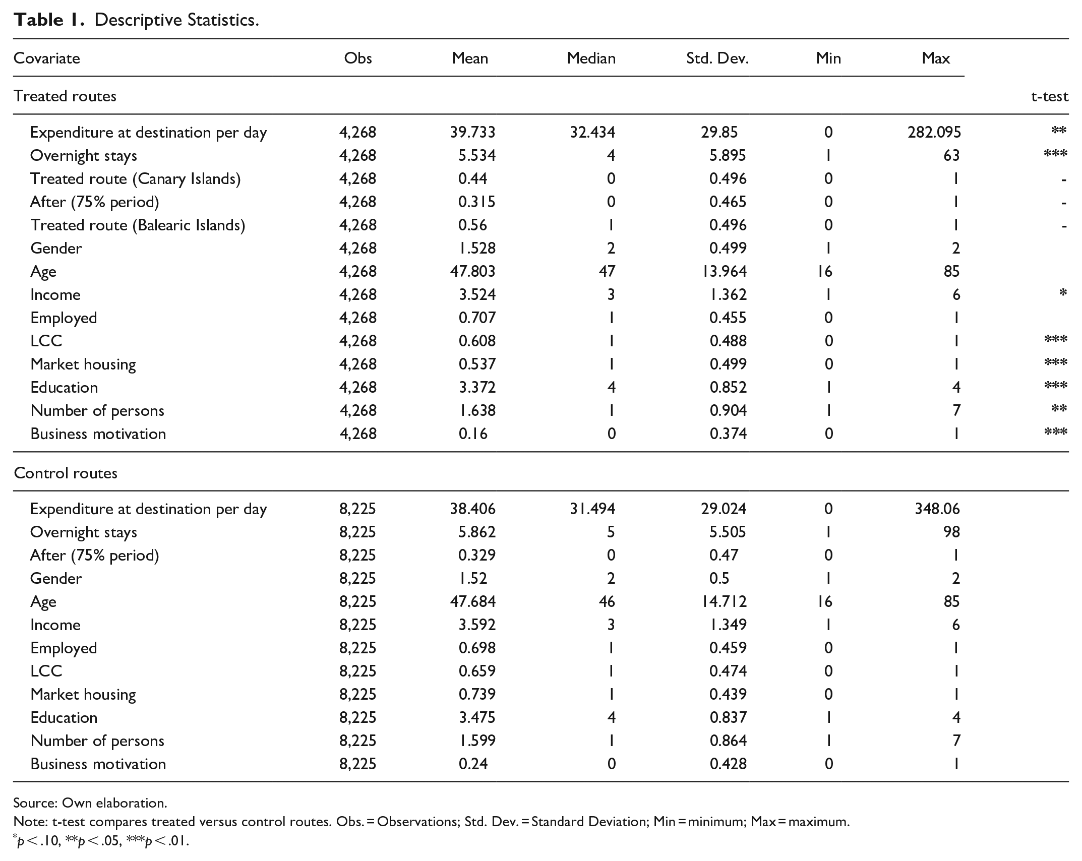
Source: Own elaboration.
Note: t-test compares treated versus control routes. Obs. = Observations; Std. Dev. = Standard Deviation; Min = minimum; Max = maximum.
p < .10, **p < .05, ***p < .01.
Methodology
DiD Estimations
Does the increase in subsidy affect the outbound tourist behavior (measured in terms of expenditure at destination per day and overnights) of residents? The DiD estimator is a technique used in regression analysis to obtain causal effects on the endogenous variable. It allows us to control for the unobserved difference on average between treated and control groups, in response to a common shock. To be able to identify this response, dummy variables for the treated routes (i.e., routes affected by the policy implementation) before and after the shock (the increase in the residents’ subsidy) are included. Mathematically the regression can be expressed as:
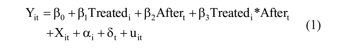
where
The coefficient
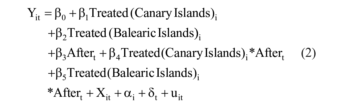
where
For the case of the overnight stays, a Hazard function was used. The parametric Hazard function has been widely used in the tourism literature for modeling the length of stay (see for instance Thrane 2012; or Barros, Butler, and Correia 2010). Model selection was generated via a multi-step procedure. In the first step, the proportional Hazard assumption was tested and rejected. In the second step, different Hazard models using accelerated failure-time (AFT) distributions (exponential, weibull, log-logistic, log-normal, and gamma) were estimated. Lastly, these models were compared by using selection criteria (AIC and BIC) and the log-normal model was preferred. It should be noted that the survival models do not have a straightforward interpretation. The output of the model can be presented as time ratio or as AFT. In the former, the coefficients should be interpreted in a multiplicative way (e.g., a coefficient of 1.10 means that the length of stay is 1.10 higher). In the latter, a transformation is needed to correctly interpret the coefficient (see subsection 5.1).
Parallel Trends
One key aspect of using DiD estimation requires that the group affected by the policy (the treatment group) and the unaffected group (the control group) had similar behavior regarding the endogenous variable. In practice, this is usually tested by analyzing the trends of both groups for the period before the “treatment” (i.e., the moment in which the residents’ discount increased). Two approaches are implemented: first a graphical analysis of trends before and after the shock; second, a statistical test.
The latter, in order to test the previous hypothesis, follows Galiani, Gertler, and Schargrodsky (2005). For this test of parallel trends, for the routes affected by the policy, the pre-treatment period is considered, but for the control group the whole period is considered. We estimate a model with no constant and that includes interactions between each group and the trend variable (i.e., the fully saturated model; so we are able to test the equality of the relevant coefficients).
Matching Analysis
Considering possible problems of unconfoundedness, exogeneity, ignorability, or selection on observables, 8 there is an alternative recommended in the academic literature when regression models have been used. While self-selection bias is removed by comparison between treated and control groups, matching analysis allows us to adjust treatment and control groups for differences in covariates, or pre-treatment variables, which is the key to obtaining the causal inference of effects, as matching analysis seeks to do (see Rubin 1974 or Rosenbaum and Rubin 1983).
Considering:

where:
Y1: outcome in the case of a unit (expenditure at destination per day or overnight stays) in the case of a unit (tourist) exposed to the treatment (change in the resident subsidy).
Y0: outcome if the unit is not exposed to treatment.
Expression (3) allows us to estimate the average effect on expenditure at destination per day or overnight stays on routes affected by the change in the resident subsidy. We are able to identify the Average Treatment effect on the Treated (hereafter, ATT), using the conditional independence assumption and a requirement for identification:
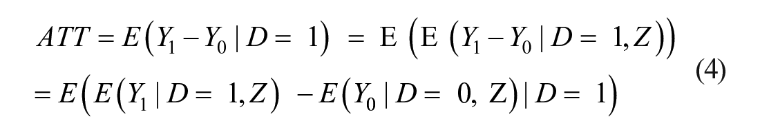
where Z is the set of observable characteristics that affect both treatment status and potential outcomes.
Results
DiD
Table 2 includes DiD results. It should be noted that all the regressions are weighted using sampling weights in order to be able to infer the results to the whole population. In all cases, F-tests were accepted at 1%. Moreover, the explanatory capacity of the models ranges from 0.45 to 0.66 and the statistical significance and sign of coefficients remain after considering the fixed effect of each model (the even estimates in Table 2). All covariates show expected signs.
DiD Estimations.

Note: Other variables included and not shown: quadratic age and binary variables for marital status. Standard errors in parentheses.
p < .10, **p < .05, ***p < .01.
Note 2: ED: Expenditure per tourist at destination per day. OLS = Ordinary Least Squares; QR = Quantile Regression.
We have to highlight three aspects of the results: the increase in the subsidy to 75% did not lead to changes in touristic expenditure at destination per day in the Canary Islands. In contrast, the increase in the subsidy does increase expenditure at destination per day and overnight stays in the Balearic Islands. Specifically, expenditure at destination per day increased by 7.5% (in QR regressions with fixed effects; although OLS was 11.2%). It should be noted that, given the test applied in subsection 5.2, the results of the expenditure at destination per day for the Canary Islands must be taken with caution since the assumption of parallel trends is rejected for this case. Thus, an alternative to check the validity of the result should be used. For this reason, a matching analysis has been implemented for the expenditure at destination per day (see section 6).
On the other hand, the interpretation of length of stay is not straightforward. The results in Table 2 have been presented in AFT metric to keep a similar format as in the expenditure result. This means that a transformation needs to be applied to interpret the result. Assuming a change of 1 unit in the covariate of interest the transformation needed is:
Our results show that tourists from both regions are affected by the policy; however, their response is heterogeneous. Nevertheless, both responses might be also explained by a positive effect of the policy over frequency, or because new passengers with shorter vacations are traveling now. However, with the current database, it is not possible to check this hypothesis due to the limitations of expenditure microdata where tourists are not followed for a particular period.
For this reason, additional data is obtained from the Spanish National Statistics Institute (INE) 9 where the number of tourists staying in market accommodation by region of origin can be obtained. Three aggregate time series are generated: people from the Canary Islands staying overnight in mainland Spain; people from the Balearic Islands staying overnight in mainland Spain; and people from mainland Spain staying overnight in mainland Spain. A structural time series analysis (see Annex 1 for further explanation) is applied to measure for any significant structural break on the level component of the time series.
The results (Table A1) show that the number of tourists from the Canary Islands to mainland Spain staying in market accommodation rose significantly (about 8.6%). However, no structural break could be found on the level component for Balearic Island and mainland Spain tourists, so there was not a significant change in the number of tourists in these last cases.
Parallel trends
Figures 1 and 2 show the average expenditure at destination per day and the average number of overnights for each month, for both the treatment and control groups. Moreover, the trend of each group is represented to be able to analyze the similarities in the evolution of the variables of interest in both groups. Ideally, the DiD estimator should be used when both the treatment and control groups have similar trends.
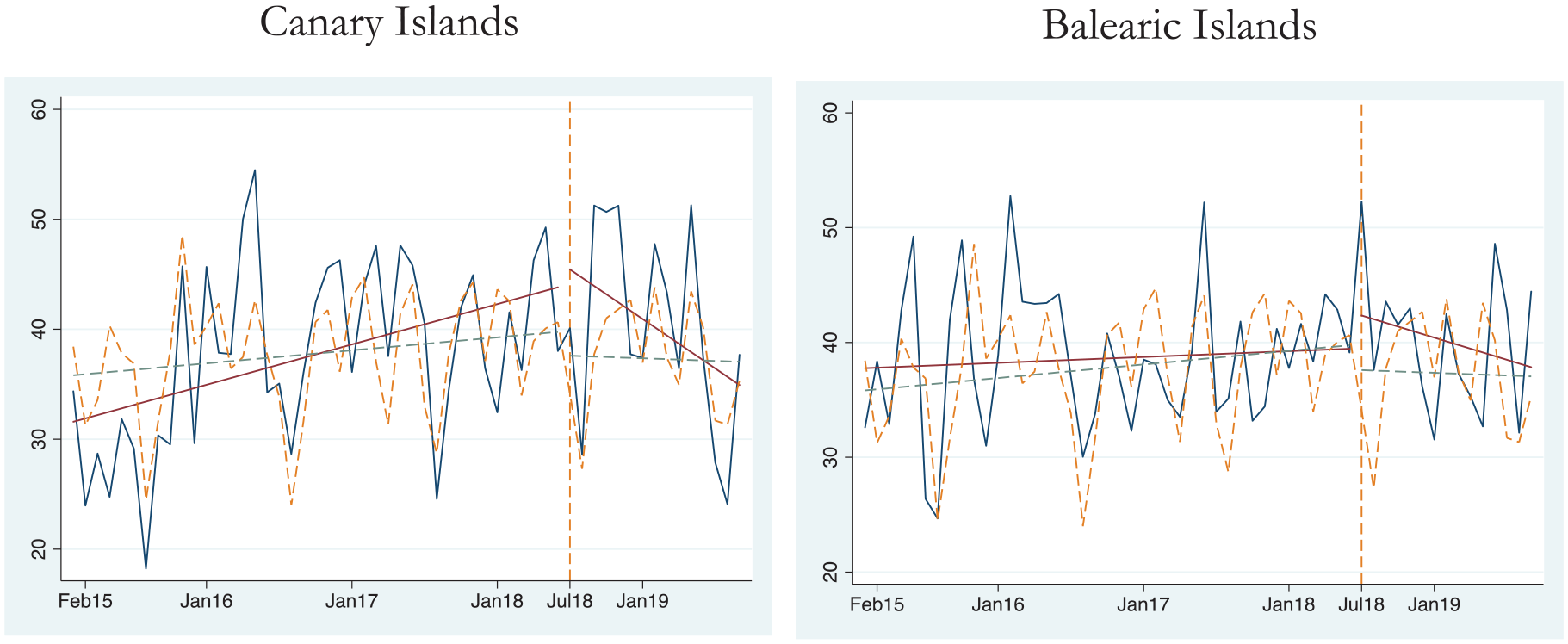
Average touristic expenditure at destination per day. Islands versus average control group.
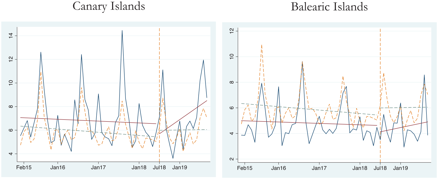
Average overnight stays. Islands versus average control group.
Figure 1 confirms that the basic assumption of the DiD estimator is not fulfilled in all figures (i.e., trends in the treated and control group are not the same in the period before the external intervention). For this reason, we test whether the outcome variables of interest (touristic expenditure at destination per day and overnight stays) follow parallel trends in both groups.
Two tests are performed for touristic expenditure at destination per day and overnight stays, for the different samples and with and without controls. One of the null hypotheses cannot be rejected (trends of the treatment and control group are the same in the pre-treatment period) in all cases, except for expenditure at destination per day in the Canary Islands. In contrast, we found for control routes before and after the intervention that the null hypothesis cannot be rejected in any case (see Table 3). This implies that the outcomes of the control group before and after the intervention had identical trends.
Parallel Trend Estimations.
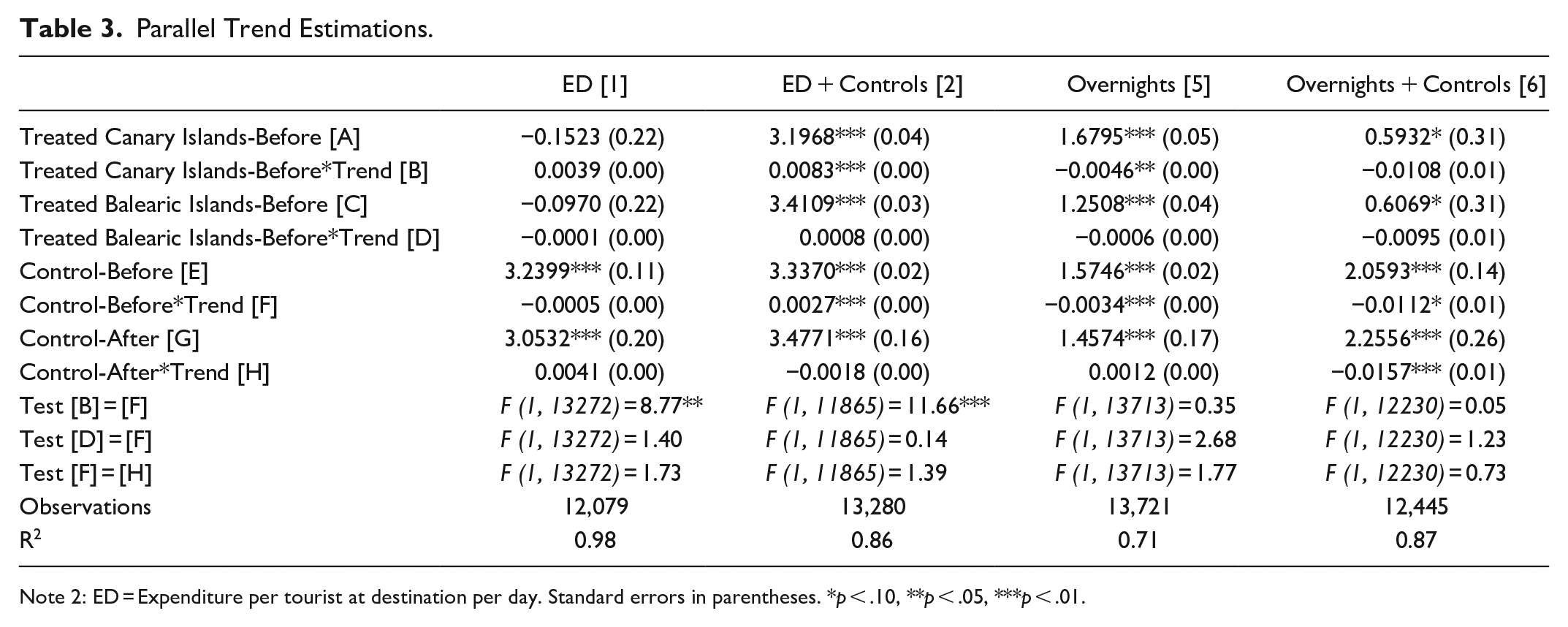
Note 2: ED = Expenditure per tourist at destination per day. Standard errors in parentheses. *p < .10, **p < .05, ***p < .01.
Our DiD identification strategy is validated except in expenditure at destination per day in the Canary Islands (so results could be biased). For this reason, we implemented a matching analysis (see below) in order to obtain the causal effect between change in the resident subsidy and expenditure and destination per day and overnight stays of resident passengers.
Matching Analysis
Given that the parallel trend assumption is not met in the data for the expenditure at destination per day for the Canary Islands, alternatives should be used in order to check for the validity of the results on this variable.
There is a significant advantage of this empirical strategy in contrast to the former one (DiD). Our unit of observation is expenditure at destination per day and overnight stays, as in previous estimations. Therefore, matching estimator pairs up the treated person, a resident tourist (who travels on routes affected by the change in the resident subsidy), with a control tourist (who travels on routes unaffected by the change in the resident subsidy) who have similar observed attributes. We repeat the procedure of comparison between the treated and control not only with the most similar pair, but with the 10, 20, and 50 most similar.
We estimate the effect of the change in the percentage of the subsidy on both endogenous variables based on all explanatory observables, but using a subsample where control routes have similar characteristics to treated routes. Therefore, the matching analysis controls for pre-existing differences between both types of routes. In this case, the explanatory variables used were the same as in equation (1) (excepting fixed effects). Moreover, according to Abadie and Imbens (2006, 2011) the nearest-neighbor matching estimator is not consistent while matching on two or more continuous variables (such as age or number of people traveling with the respondent). Thus, the authors recommend a bias adjusted estimation while linearly regressing over the continuous variables. This model was estimated using STATA. 10
Table 4 shows that the results support the main conclusions derived by DiD estimations: the increase in the subsidy from 50% to 75% increases touristic expenditure at destination per day for those residents in the Balearic Islands (from 11.9% to 16.3%) but not those in the Canary Islands. These results are similar in both the sign and value of the coefficients and the significance of the parameters, supporting the results of the DiD models obtained before.
Summary of Results of the Matching Estimator.
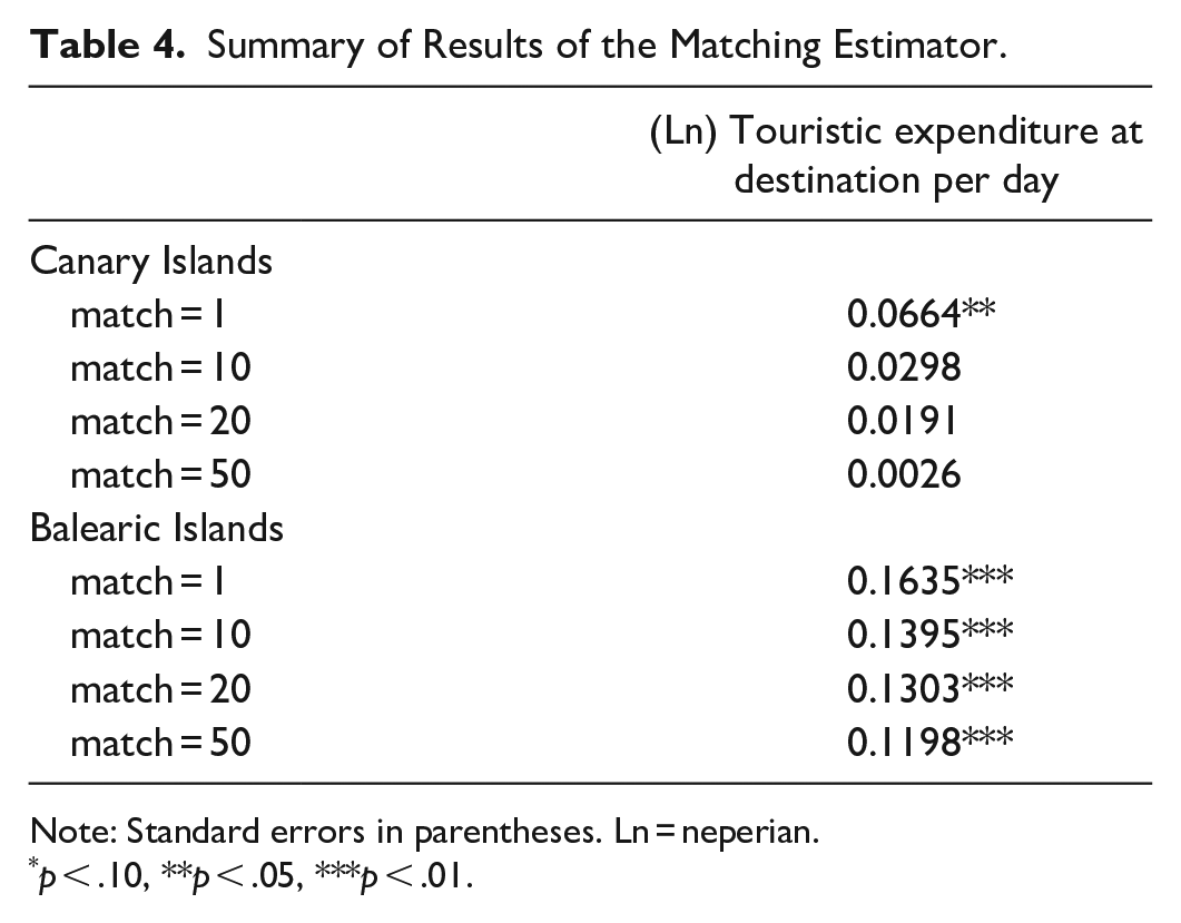
Note: Standard errors in parentheses. Ln = neperian.
p < .10, **p < .05, ***p < .01.
Additionally, the robustness of the results has been validated by applying two different placebo tests. On the one hand, we applied the DiD estimation to a different date. On the other, we applied the DiD estimation to tourists from other two randomized selected regions. The results of these tests showed that our estimations are robust (the DiD variables of the placebos was not significant) and can be seen in Annex 2.
Discussion
To our knowledge, this is one of the first papers to analyze the effect of a subsidy to affected consumers in tourism by analyzing its causal effects on daily expenditure and length of stay. The lack of existing literature with a similar approach makes comparison with other studies complicated.
First, our structural time series model shows that after the change in the subsidy the number of total arrivals from the Canary Islands to mainland Spain increased. This result aligns with the existing literature where subsidies are associated with an increase in demand (see for instance Chow, Tsui, and Wu 2021; or Matsuura and Saito 2022). Nevertheless, it should be noted that our results (and also results of the existing literature) cannot differentiate the source of the demand increase (i.e., the available data makes it impossible to distinguish between the increase in trips of existing travelers, from new travelers that did not travel before the policy implementation). However, in the case of the Balearic Island tourists, this result does not apply. One plausible explanation of this disparity is the difference in transport costs. Assuming that the transport costs are positively related to distance, which is usually assumed in demand analysis (see for instance Peng, Song, and Crouch 2014), the Balearic Islands is closer than the Canary Islands to mainland Spain and journeys between them were more common, so the policy was insufficient to increase average frequency or generate new tourists.
Second, analyzing daily expenditure, the existing literature showed that price ticket savings of LCC were partially invested in the destination (Eugenio-Martin and Inchausti-Sintes 2016; Ferrer-Rosell, Coenders, and Martínez-Garcia 2015; or Gómez-Déniz and Perez-Rodriguez 2021). However, regarding these studies, it was not possible to conclude if this was related to the low-cost passenger tourist profile or if it was a general result. The policy studied in this paper has been applied to all tourists, whatever the airline, or even the fare class. Our results again show mixed results. In the case of tourists from the Canary Islands, there is no significant difference in terms of expenditure at destination per day. However, tourists from the Balearic Islands do increase their expenditure at destination per day.
Third, our results show that both, tourists from the Balearic Islands and the Canary Islands reduce their length of stay after the policy. According to Gössling, Scott, and Hall (2018), the reduction of length of stay is a global phenomenon. However, even assuming this decreasing trend of length of stay, the DiD estimator yields to causal results, because it compares treated versus control group. This means that even if all the destinations were reducing their length of stay, the treated regions are decreasing at a higher level, due to the change in residents’ subsidy.
Finally, taking all results together, we can draw interesting conclusions. Tourism behavior has changed due to the policy. However, these changes are not homogeneous. One plausible explanation for these differences is the distance from the origin markets to the destinations, which is positively related to travel costs. This means that while the policy clearly modifies tourist consumer behavior, these changes are different depending on the travel costs. For tourists from the Balearic Islands, which are close to the mainland destinations (1 hour 20 minutes and 50 minutes from Palma to Madrid and Barcelona respectively, by plane), their behavior changed to shorter, but with higher daily expenditure, vacations. On the contrary, tourists from the Canary Islands, who are far from mainland destinations (2 hours 50 minutes and 3 hours 20 minutes from Tenerife Norte to Madrid and Barcelona respectively) also opted for shorter vacations, but increased their demand without any significant change in their daily expenditure. However, as we have explained, it is not possible to differentiate between higher frequency and newly generated demand. These heterogeneous results contrast with Jiménez, Valido, and Pellicer (2021), who analyzed the effect of this air transport subsidy to non-residents. They found a clear negative effect of mainland tourists traveling to the archipelago in both length of stay and daily expenditure.
Conclusions
This paper analyzes the effect of an increase in the percentage of subsidies enjoyed by residents in the Canary and Balearic Islands on their expenditure at destination per day and overnight stays when they fly abroad. In order to address this question, both a DiD estimator (using both OLS and Quantile regression) and matching procedures have been taken. Moreover, we perform several robustness checks and placebo tests.
Although AIReF (2020) showed that there was an increase in air transport ticket prices from the Canary and Balearic Islands to mainland Spain after this change, this increase was insufficient to net out the increase in residents’ discounts. Thus, these passengers enjoyed lower net ticket prices. Our results show that, after the policy implementation, the effects of this net ticket price reduction for residents were not homogeneous, and generated a different response in each target region.
First, expenditure at destination per day in the case of the Balearic Islands has increased, meaning that tourist travelers from the Balearics to mainland Spain spent more at destination after the subsidy increase. However, the same causal effect could not be found in the case of the tourist from the Canary Islands, meaning that there is no trade-off between air transport savings and expenditure at destination per day in this case.
Second, in terms of length of stay, we found a homogeneous response to the policy in both cases. It was shorter in both archipelagos, meaning that tourists affected by the policy not only have not extended the length of their stay, but chose a shorter vacation; so the policy has changed the average pattern of the tourist. Plausible explanations for this behavior include that these tourists are traveling more frequently, there are new tourists traveling, or both.
Finally, an analysis at macro level allowed us to contrast the hypothesis about the number of trips being increased. Our results also showed a heterogeneous response to the policy at each archipelago. The number of trips rose for Canary Island tourists (+8.6%) while they remained unchanged for those from the Balearics. This means greater travel frequency and/or new demand generation by Canary Island residents, but not for those from the Balearic Islands.
Analyzing these results together, we cannot conclude that total expenditure is rising because of the subsidy change. On the one hand, the impact in total expenditure per travel and total expenditure is ambiguous for the Balearic Island tourist as they impact on each of the dimensions studied differs. On the other, the impact on total expenditure per trip for the Canary Island tourist diminishes, as they spend the same but stay less days at the destinations. However, as the number of tourists rise, the effect on total expenditure is unknown.
In short, increasing residents’ air transport subsidies do not necessarily improve total expenditure for outbound tourism. Thus, as air transport subsidies is a policy applied in a number of countries to promote territorial equity (Spain, Italy, France, and Portugal, for example), further research should be conducted on the topic if better data becomes available in order to fully understand the net impact of this policy.
While this study is one of the first to analyze the implications of a ticket price reduction affecting all passengers instead of only a particular group (e.g., LCC passengers), some methodological constraints limit the analysis. The first is that the data is not “proper data” (i.e., where tourists are followed for a particular period, but has been formed through several cross sections). This problem, analogous to other publicly available surveys analyzing tourist expenditure, does not allow for the measurement of flight frequency. Thus, we encourage policymakers to improve public data collection to allow researchers to measure the three dimensions: expenditure, length of stay and frequency of flights. Finally, we wish to clarify that the COVID-19 pandemic only affected our study by limiting the post-policy time frame, which is not included in our database.
Footnotes
Annex 1. Structural Time Series Model
The Structural Time Series Model (STSM) Harvey (1989) disentangles a time series into its unobserved components (level, slope, seasonal, cycle and irregular). These models are usually used for forecasting. However, they can be also used to analyze the structural change in time series derived from particular events. There are three types of interventions in these models. Firstly, interventions in the irregular component, which are related to outlier observations. Secondly, slope interventions, which imply a change in the growth rate of a time series after a particular event. Lastly, level intervention, which is related to level shift on the time series after a particular event. To analyze the impact of air transport subsidy on the number of tourists, a level intervention was tested. A significant level intervention means that after the policy, there was a significant shift in the average number of monthly tourists that produced a structural change in the series. Moreover, the STSM allow for a multivariate specification, which implies that the time series are related by the error term in a similar way as the Seemingly Unrelated Regression Equations (SURE) (Commandeur and Koopman 2007). Mathematically the model can be expressed as:
Equation (A1) represents the observation or measurement equation, where
where
Equation (A2) represents the transition equation, where µ
The results of the model are shown in Table A1.
Annex 2. Robustness Checks for DiD
We perform two different standard placebo tests already used in the literature, changing the period of the exogenous intervention and changing the treated regions. That is, in the first placebo test, we repeat the estimations but only in the period before the exogenous change in order to check if there are the same effects of the resident subsidy change in the variables (expenditure at destination per day and overnight stays). In the second case, we substitute the Canary and Balearic Islands for other regions. With these two tests, we are able to ensure that the effects found are due to the change in the subsidy, and not for other reasons or missing variables.
Acknowledgements
The authors are thankful for the comments and suggestions received from Juan Luis Eugenio-Martín and Federico Inchausti and the anonymous referees. The usual disclaimer applies.
Declaration of Conflicting Interests
The author(s) declared no potential conflicts of interest with respect to the research, authorship, and/or publication of this article.
Funding
The author(s) received no financial support for the research, authorship, and/or publication of this article.