A Sequential Pattern Mining Approach to Tourist Movement: The Case of a Mega Event

Abstract

The movement of tourists has important economic and social implications for destination management. However, tracking and analyzing such movement can be a challenge both conceptually and methodologically. Using four different sequential pattern mining algorithms, this study investigates the movement of international visitors during the Gold Coast Commonwealth Games (GC2018) at the level of a specific destination through Twitter data. Results indicate that sequential pattern mining is a powerful technique to reveal complex travel patterns and provides insights into the potential associated destinations of visitors beyond the current point-to-point analysis. This approach can assist destination management and event organizers in identifying the event’s contribution to tourists’ local visitation.

Keywords

gold coast sequential pattern mining Twitter tourist movement mega event

Introduction

The concept of tourist movement or dispersal has been frequently used to examine the propensity of visitors to venture beyond the gateways within a host destination (Koo, Wu, and Dwyer 2012). Since a destination could be defined at different geographical levels, tourist movement could refer to the extent that inbound tourists disperse beyond gateway cities to regional areas at a national level, or the extent that tourists disperse beyond the central attractions in a given city to its peripheral areas at the local level (intra-destination level). Studies on tourist movement, particularly tourist dispersal are important (Edwards and Griffin 2013; Hardy, Birenboim, and Wells 2020), as tourist movement defines the locations of tourist expenditure and how they contributable to the economic impacts in sub-regions (Koo, Wu, and Dwyer 2012). The greater the tourist dispersal, the wider the distribution of economic gains in the local community (Hardy, Birenboim, and Wells 2020; Wu and Carson 2008). In addition to understanding the economic impact, investigations into tourist movement improve our understanding of visitor experiences (Sørensen and Sundbo 2014), help crowd management (Hallo et al. 2004), and aid planning and adjustment of transport systems (Edwards and Griffin 2013).

Tourist movement has resurged as a topic of inquiry in recent years due to the increasing recognition of its economic and social impact on destination development, providing tourism practitioners with information on how and where to improve product development and destination planning (Hardy, Birenboim, and Wells 2020). Prior studies have demonstrated that accurate and timely information of tourist travel patterns and behaviors can assist the planning, refinement, and implementation of attractions and marketing strategies for host organizations and communities (Edwards and Griffin 2013), identify barriers and bottlenecks for planning (Prideaux 2000), help with the return on investment (Vu et al. 2018), identify the right travel packages for different tourist segments (Xia, Zeephongsekul, and Packer 2011) and encourage more equitable distribution of tourism income (Hardy, Birenboim, and Wells 2020).

While significant progress has been made in the past two decades both methodologically and conceptually, there still exists a limited understanding of how tourist movement occurs in a temporal space during a mega event, as these attract a significant number of international and interstate visitors whose behavioral patterns can be different from regional and local tourists. Mega events can significantly influence tourist movement as the daily program and activities influence tourist behaviors (Fourie and Santana-Gallego 2011). More importantly, mega events’ economic and non-economic impacts go beyond the events themselves to benefit the surrounding regions and the host country at large, because attendees often explore not only the host city but also the region and country before and after the event period (Mair et al. 2021). For this reason, governments have sought to capitalize on mega events to develop and stimulate tourism to achieve economic development and social transformation (Wang and Jin 2019).

Therefore, tourist movement is important for the host cities of mega events, as it can help estimate the economic, social, and environmental impact of these events. The 2018 Commonwealth Games held on the Gold Coast of Australia in the state of Queensland (GC2018) was chosen as a case study. Mega events of this nature attract a significant number of domestic and international visitors, presenting an ideal event context to understand the dispersal of the visitors during the game time. Traditional methods examine tourists’ movements by recruiting respondents to use tracking apps and surveys. However, these methods might not be readily applicable in the case of GC2018. The Gold Coast is not a major gateway city and tourists can visit the events through various transport modes. This presents a major challenge in understanding tourist movement during a specific event. As such, an alternative approach is required to deal with this challenge, such as the sequential pattern mining approach using social media data instead. Sequential pattern mining is a structured data mining approach, which is used to identify the statistical correlated patterns between the data values in a sequential order (Mabroukeh and Ezeife 2010). Essentially, sequential pattern mining, as explained in more detail later in the paper, statistically assembles pieces of past visitors’ journeys and creates predictions of what tourists with similar profiles are likely to do next. Therefore, this study utilized a novel and innovative analytical approach integrating four sequential rule mining algorithms (i.e., TopSeqRules, TNS, TruleGrowth, and ERMiner) to identify tourist movement through a geographically informed filtering process. It aims to:

(1) Propose a more comprehensive sequential patterning mining approach to understand tourist movement during a mega event;

(2) Evaluate the effectiveness of the proposed approach through a case study of GC2018 using geo-tagged Twitter data within a specific destination.

The current study offers conceptual and methodological contributions to the extant tourism literature. Theoretically, our study extended the tourism movement literature by conceptualizing the transit area—it is not a place simply based on transport network alone but is influenced by a range of factors including event scheduling and destination attractions. This directly addresses the call by McKercher, Filep, and Moyle (2021) to consider the seemingly continuous failure to acknowledge the concept of time expenditure, that is the tradeoff between the time spent in transit and at an attraction or event and where the creation of transit areas can be a scarce resource. Methodologically, using a combination of four different algorithms, our study advances on the existing tourist movement literature by offering a more systematic and objective overview, serving as a potential new approach for future research in understanding this phenomenon through social media data. In particular, the study offers an empirically validated set of guidelines for tourism researchers on how to create a systematic and accurate predication of tourist movement patterns. Compared to traditional methods, our proposed approach allows for the examination of tourist movement at lower cost and with greater flexibility and predictive power, enabling the discovery of additional insights that would not otherwise be possible.

Literature Review

Tourist Movement

Tourist movement has been a relatively well-studied phenomenon in the tourism literature. Much of the focus is on national/international gateways to regional areas and how this movement is an important means of economic growth for regional development. More recently, with over-tourism being discussed worldwide, increasing voices point to the urgent need for tourist dispersal into regional areas to diversify tourism offerings, reduce congestion in popular tourist destinations, and improve the distribution of tourism benefits nationwide (Hardy, Birenboim, and Wells 2020). The economic and social-cultural benefits have also been documented in various government and regional organizations’ strategic plans.

Tourist dispersal is generally conceptualized as the movement of tourists from a tourism center to places that are less known with more modest and limited tourism facilities. Initial conceptualizations were based on a core and periphery principles. Since then, the concept has gone on to incorporate flexible classification systems at various scales from a global, national and specific destination level (Chen, Becken, and Stantic 2021). Studies on tourist dispersal (e.g., Edwards and Griffin 2013; Hardy, Birenboim, and Wells 2020; Wu and Carson 2008) have largely focused on two streams. The first stream identifies the factors that influence tourist dispersal. The commonly identified factors include two main areas. The first is related to the characteristics of the tourists, such as length of stay (Hardy, Birenboim, and Wells 2020), cultural background (Wu and Carson 2008), travel party composition (Koo, Wu, and Dwyer 2012) and whether the tourists are first-timers or return visitors (second, third time) (McKercher et al. 2012). The second is related to the destinations themselves, including types of transport available (Koo, Wu, and Dwyer 2010), the distance between tourist attractions (Mckercher and Lau 2008), and weather (Becken and Wilson 2013). These studies, while highlighting common factors, present contradictory findings (Hardy, Birenboim, and Wells 2020). For example, the effect of weather on tourist dispersal has been argued by Becken and Wilson (2013) as an important factor, whereas McKercher et al. (2015) argue that it plays a more minimal role.

The second stream focuses on exploring travel itineraries and patterns. Studies have shifted from an early conceptualization of travel patterns, such as the Travel Dispersal Index to empirical studies that identify tourists’ travel movements between countries and destinations (Hardy, Birenboim, and Wells 2020). While increasing studies on travel patterns provide empirical insights into tourist dispersal, researchers have put considerable effort into exploring various approaches to better identify tourist dispersal patterns.

Early studies on tourist dispersal typically use conventional data collection methods, including observations, post-visit questionnaires, interviews, recall maps, and movement diaries (e.g., Gu et al. 2021; Hardy, Birenboim, and Wells 2020). Information on visitor (tourist) spatial distribution is also provided by various statistical agencies such as the Australia Bureau of Statistics (ABS) and Tourism Research Australia (TRA) that collect data on international arrivals, departures, and expenditures (Koo, Wu, and Dwyer 2012; Koo, Lau, and Dwyer 2017). ABS arrival data are relatively accurate, but further insights on how tourists move within a country are not available. TRA’s international visitor survey (IVS) and other tourism dispersal studies typically employ traditional data collection methods such as questionnaires, which require face-to-face contact with tourists and can suffer from the various problems associated with survey research such as response rates, coverage, recall bias and missing data (Couper 2000). They are also limited in terms of scale of geographical locations with their focus being restricted primarily to major gateway cities. There are also few cross-references made between geographic locations and tourist behaviors (i.e., what tourists did at which locations). As such, these studies are limited in terms of the quality of the response rates and scales of geographical locations (Vu et al. 2018).

Researchers continue to use geoinformatics to understand tourist dispersal by using global positioning system (GPS) tracking and mobile/app-based approaches. These studies have enabled a more detailed and accurate understanding of tourist dispersal at a destination level including the development of various indicators to measure tourist dispersal. Hardy, Birenboim, and Wells (2020) proposed and empirically examined three key alternative approaches (maximum distance traveled, total distance traveled, and activity space) to measure tourist dispersal in the Australian island state of Tasmania finding that these analytic approaches can be effective based on different purposes to measure tourist dispersal. More recently, researchers have begun to utilize user-generated content to understand tourist movement by scaling the sample and by offering of more advanced methodological approaches (Vu et al. 2015, 2018). Hardy, Birenboim, and Wells (2020) highlight in their most recent study that there is no universally applicable approach but each has its own merits for understanding tourist dispersal. Indeed, these studies have laid a solid foundation for understanding tourist dispersal and call for a more advanced methodological approach to complement existing analytic methods.

From a geographical perspective, existing studies have examined dispersal at the national level by employing visitor survey data. For instance, Wu and Carson (2008) identified aggregated visitor travel patterns over multi-destinations. Some studies further combined survey data with GPS to understand visitor behavior (e.g., East et al. 2017). However, research on dispersal at a single destination level (intra-destination) is limited. Bauder and Freytag (2015) produced one of the few such studies which found that visitor mobility in a city relates to their pre-trip preparation—well-prepared tourists visit places outside of the inner city with a wide range of activities. Table 1 presents various research methods from representative studies on tourist movement.

Table 1.

Tourist Movement Data Collection Approaches.

Methods to Collect Data	Advantage	Drawback	Analytical Approach	Examples of Study
Traditional methods (e.g., observations, post-visit questionnaires, interviews, recall maps, and movement diaries)	More participant variables and attributes can be identified	Biased findings; high operating costs; limited updates and sample size; limited scales of geographical locations	ANOVA	Gu et al. (2021)
Tracking methods (e.g., mobile phone signal, GPS and GPS-enabled mobile applications, Wireless Fidelity [Wi-Fi and Bluetooth])	Larger spatial area; monitor movement; record tourist origins; not weather-dependent; produces precise, reliable, accurate, and continuous data	Limited access; limited user’s profile due to data privacy; data associated with graphs and metrics	Time geography; mining of association rules; binary logistic regression; intersection and frequency analysis	East et al. (2017), Gu et al. (2021), Shoval et al. (2020), Raun, Ahas, and Tiru (2016), and Versichele et al. (2014)
Online platforms/reviews	Target users and providers; relatively easy access; larger scale	Limited profile details; data reliability due to fake reviews	Content analysis; social network analysis	Leung et al. (2012) and Zeng (2018)
Social media platforms (e.g., Flickr, Weibo, Twitter)	Access to user’s profile and geotagged information; larger scale; constant availability of user-generated data	Require advanced analytics methods	Sequential pattern mining; Sankey diagrams; geographic information systems; trajectory mining and tourist detection	Chen, Becken, and Stantic (2021), Chua et al. (2016), and Vu et al. (2015, 2018)

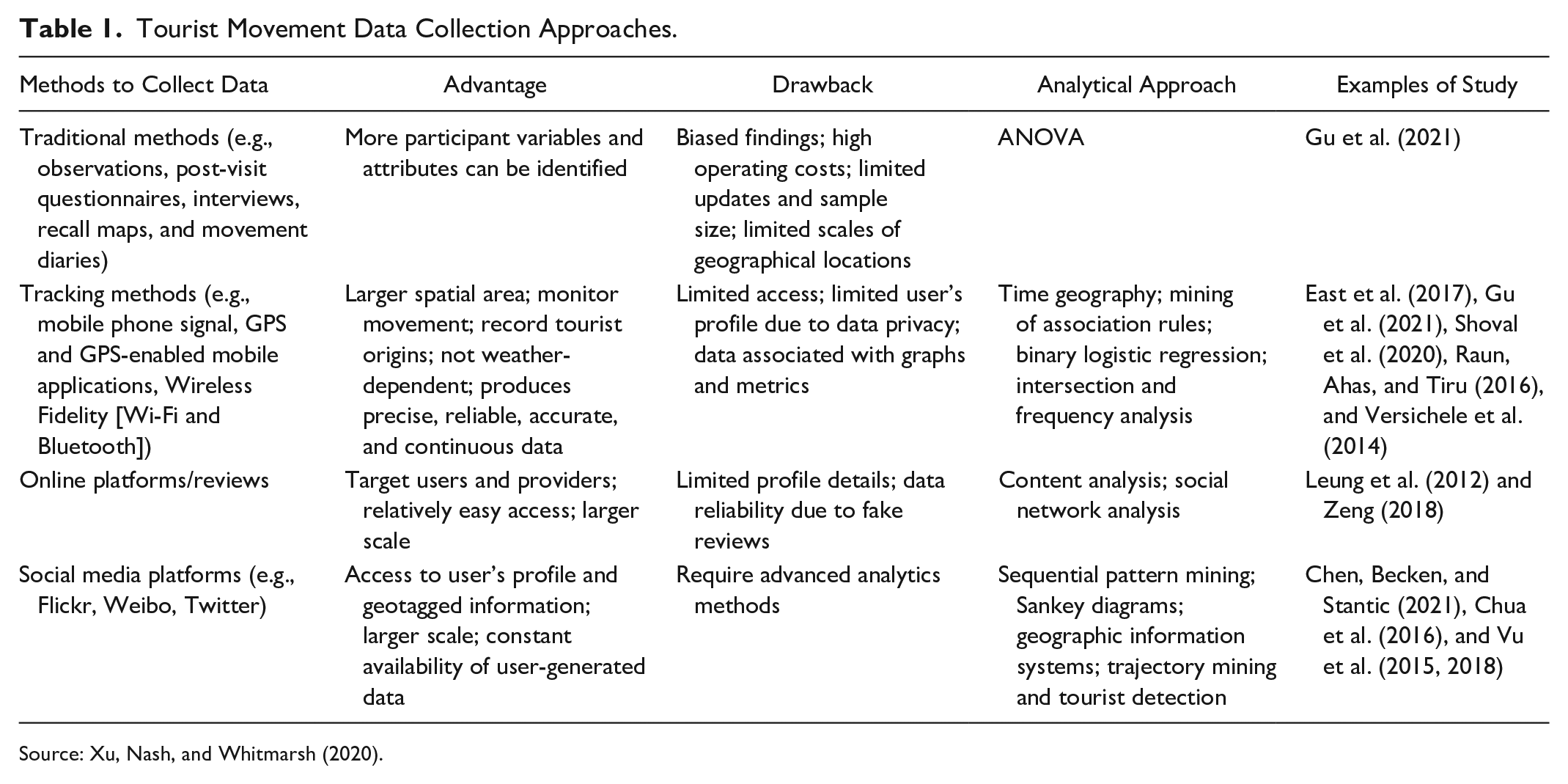
Source: Xu, Nash, and Whitmarsh (2020).

Within the event context, studies on tourist movement are rather limited, with a heavy focus on outdoor events using GPS devices or/and questionnaires (East et al. 2017; Pettersson and Getz 2009; Pettersson and Zillinger 2011). For example, Pettersson and Getz (2009) has considered tourist movement in the event context but it is limited to the host village and four event areas, rather than a whole destination, and it employs traditional methodological approaches based on observation and interviews. While these studies provide important insights into managing congestion, crowding, and hazardous situations in events, it remains unclear how the tourists moved over time during a mega event at the destination level, apart from their event experience.

Sequential Pattern Mining

Sequential pattern mining is a structured data mining approach, which is used to identify the statistical correlated patterns between the data values in a sequential order (Mabroukeh and Ezeife 2010). The input of a sequential rule mining algorithm is a set of sequences S = {s₁, s₂, . . ., s_s} and a set of items I = {i₁, i₂, . . ., i_t} contained in these sequences. Each sequence is assigned a unique sequence id (sid) and is a list of item sets ordered by time, denoted as s_x = <I₁, I₂, . . ., I_n> such that I₁, I₂, . . ., I_n ⊆ I, where an itemset contains one or more items that are considered to appear at the same time (Fournier-Viger and Tseng 2011). For example, a sequence s₁ = <{1}, {2, 3, 4}, {3, 5}, {6}, {5, 6}>, contains five item sets. Item one is followed by items 2, 3, and 4 at the same time, which are followed by 3 and 5, followed by six, and then followed by 5 and 6.

The purpose of sequential rules is to identify rules of the form X ==> Y, a relationship between two disjoint and unordered item sets X, Y ⊆ I, meaning if some items × appear, they will be followed by items Y (Fournier-Viger and Tseng 2011). Thus, the sequential rule indicates that something (Y) will happen after something else (X). Also, if there is a sequence with a single itemset, then it is impossible to find a sequential rule because all items in that sequence are assumed to be simultaneous (Vu et al. 2018). As such, only when there are at least two itemsets, can the rules be identified.

A sequential rule X ==> Y typically has two properties: Support and Confidence. Support is equal to the number of sequences where X appears before Y, divided by the total number of sequences; Confidence is calculated by dividing the number of sequences in which X appears before Y by the number of sequences in which X appears (Fournier-Viger et al. 2015). These two measures reflect the frequency and confidence of the sequential rule X ==> Y in the sequential database, and are computed based on equations (1) and (2) respectively. Generally, the range of Support and Confidence is from 0 to 1. The greater their values are, the better the performance for discovered rules will be. Also, traditionally, sequential rule mining is to identify all rules with Support and Confidence not less than the specified minimum Support (minSup), and the specified minimum Confidence (minConf) (Fournier-Viger et al. 2012a).

Support (X == > Y) = | s i d s (X == > Y) | / | S |

(1)

Confidence (X == > Y) = | s i d s (X == > Y) | / | s i d s (X) |

(2)

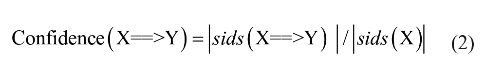
Where sids (X ==>Y) denotes the set of sequences where the rule appears; sids (X) indicates the set of sequences where all the items of X appear.

In practice, it is not easy to specify minSup and minConf. MinSup should be specified considering the characteristics of the sequential database, whereas minConf can be selected depending on the user. There are not enough rules when minSup is too high, and performance deteriorates when minSup exists too low (Nguyen et al. 2017). Thus, several algorithms discovering the top-k most frequent sequential rules have been developed in the past decade, such as TopSeqRules (Fournier-Viger and Tseng 2011) and TNS (Fournier-Viger and Tseng 2013). The TopSeqRules algorithm solves the problem of hard setting minSup by allowing users to directly input k, which is the amount of rules to be identified (Fournier-Viger and Tseng 2011). As such, the TopSeqRules algorithm is exact, and it will find all the rules meeting the constraints set by the k and minconf parameters. However, a problem with the TopSeqRules algorithm is that it can discover rules that appear to have some kind of redundancy (Fournier-Viger and Tseng 2013). For example, rule X ==> Y and rule X ==> Y, Z, can have exactly the same Support and Confidence score, and thus one of them can be randomly abandoned. To avoid this problem, the TNS algorithm is proposed to identify the top-k most frequent non-redundant sequential rules, and works exactly in the same way as the TopSeqRules algorithm. The difference is that TNS eliminates some redundant rules (Fournier-Viger and Tseng 2013).

In addition to the given Support and Confidence, some algorithms can be used to optimize the generation procedure of sequential rules. The TruleGrowth algorithm, an extension of the RuleGrowth algorithm, generates rules one item at a time, discovers temporal rules with a sliding window constraint to satisfy users’ need to seek rules occurring within a maximum time span for many real-life applications (Fournier-Viger et al. 2012b, 2015). Further, the TruleGrowth algorithm performs better in memory scalability than the RuleGrowth algorithm, which means that if the amount of data is increased for the TruleGrowth algorithm, memory usage will increase more slowly than if we increase the data volume to the RuleGrowth algorithm (Fournier-Viger et al. 2012b). Memory scalability refers to how much the memory usage will increase when we increase the amount of data as input to an algorithm. For example, when we increase the amount of data, the memory could increase a little, increase linearly, increase exponentially, etc. So to evaluate the memory scalability, we varied the size of the dataset for an algorithm and checked how much memory was used. When memory usage increases exponentially, it presents a data processing problem. Ideally, memory usage increases linearly with the size of the data. Another variation of the RuleGrowth algorithm is the ERMiner algorithm which promotes performance in identifying rules by applying the data structure named SCM (Sparse Count Matrix) and the equivalence classes (Fournier-Viger et al. 2014a). As such, it can be faster to find rules that appear in dense or long sequence databases, but it also consumes more memory.

In short, these algorithms have their own strengths and weaknesses in the discovery of sequential rules occurring in a sequence database with different procedures, strategies, and parameters. The current study employed TopSeqRules, TNS, TruleGrowth, and ERMiner for mining efficient travel sequential rules.

Case Study

The Research Setting: GC2018, Venues, and Points of Interest

The case destination is the Gold Coast which is a city in the Australian state of Queensland with a population of 540,000. It is a popular holiday destination for domestic and international tourists, which has become famous for its beaches, year round warm to hot climate and theme parks.

GC2018 was held in a regional center, providing an ideal context to understand tourist dispersal. Held every four years, the Commonwealth Games is an international sports event involving Commonwealth Nations athletes. GC2018 attracted more than 4,000 athletes from 71 Commonwealth Games Associations and was watched by an estimated 16 million viewers in Australia and 1.5 billion viewers worldwide (Queensland Government 2018). GC2018 opening ceremonies were held on 4 April and the closing ceremonies on 15 April 2018. The main venues for the games listed according to their geographical locations include: (1) Nerang area—Carrara Stadium for opening and closing ceremonies and Athletics, Carrara Sports and Leisure Centre for badminton, weightlifting, wrestling, (2) Broadbeach—Broadbeach Bowls Club for lawn bowls, GC Convention and Exhibition Centre for netball and basketball, (3) Southport—Optus Aquatic Centre for swimming and diving, Southport Broadwater Parklands for Triathlon and Athletics, Gold Coast Hockey Centre for hockey, (4) Coomera Indoor Sports Centre for gymnastics, netball, Oxenford Studios for boxing, squash, and table tennis, (5) Robina—Robina Stadium for Rugby Sevens, (6) Coolangatta Beachfront for Beach volleyball. During the games public transport use (esp via light rail) was encouraged along with park “n” ride facilities, and shuttle buses were made available (see Figure 1).

Figure 1.

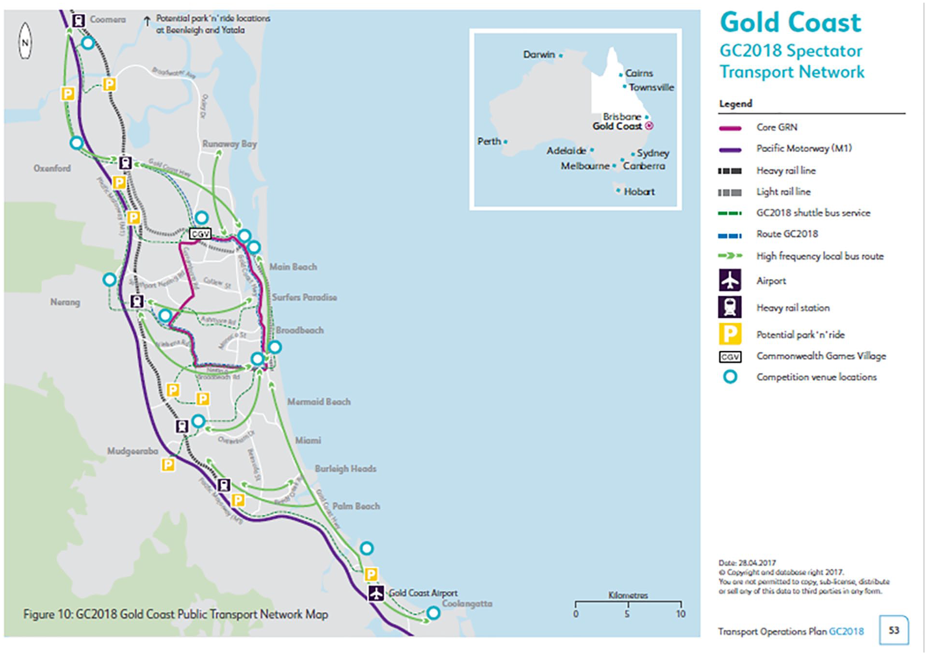
GC2018 spectator transport network.

Methods

This research takes an inductive (bottom-up) approach by: (1) collecting and analyzing social media (Twitter) data, (2) identifying patterns and relationships from the analysis of the results, and (3) proposing explanations to the identified patterns toward the end of the research process.

Data collection and cleaning

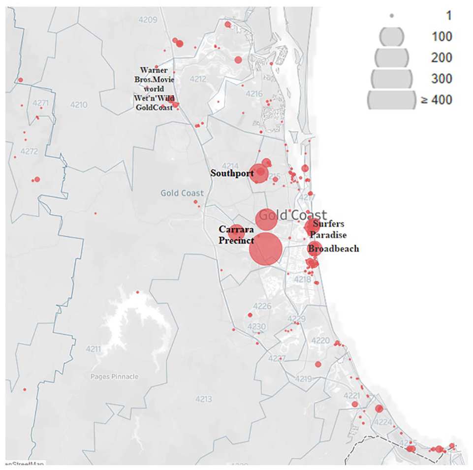
Twitter data was used in this research to analyze international visitors’ dispersal within and beyond the Gold Coast during the Commonwealth Games. The key advantage of Twitter data is that tweets are publicly available on a large scale with geo-tagged information providing an ideal means to capture attendee travel patterns (Jin and Cheng 2020). We captured twitter data within a 20 km radius of Surfers Paradise (which is at the center of Gold Coast 28.000719, 153.427269). We extracted twitter data daily during the period of the games capturing 377,960 tweets in total, which contained the terms “GC2018” or “games” posted within the area. About 1.87% of the data (7,087 tweets) provided exact location points. While 7,087 tweets with coordinators might seem small, it is not uncommon in tourism research when using social media data as not all of the information from the social media data can be used in addressing specific research questions. Figure 3 shows the number of users per suburb. Key information collected included: (1) user Id, which was used to identify unique users, (2) tweet post location, that identified where posts were generated, (3) tweet time to detect the travel sequence, and (4) user bios, which contained the city or countries that the user listed as his/her current location, which was used to identify visitors as either domestic or international.

For the purpose of this research, we only examined international visitors’ movement at the Gold Coast. The rationale for not examining domestic visitors is that methodologically, we were unable to distinguish domestic tourists and local residents through their bios. Therefore, only Twitter user locations outside Australia were included. To better understand the dispersal of international visitors, only tweets with geographic coordinates (Latitude and Longitude) were retained for sequential pattern mining, resulting in 1,887 tweets with both international profiles and geo-tagged information for future analysis. Further, three travel observations and one user were also removed from the data as their coordinates fall outside the boundary of the Gold Coast, resulting in a data set of 1,884 travel observations from March 17th to April 25th, 2018.

The use of social media data in general to track tourist behavior always entails ethical consideration (Caldeira and Kastenholz 2020). Extant research suggests that social media data can be used—within the confines of ethical research practice—as long as the content is public, there is informed consent, anonymity is ensured, and no risk or harm would come to the researchers or the twitter users (Chen, Becken, and Stantic 2021; Epstein and Quinn 2020; Townsend and Wallace 2016). In this study, only Twitter data that was publically available and that the publication of any content from users had been consented to by the use terms set by Twitter was used. The following quote taken from Twitters Rules notes “most content you submit, post, or display through the Twitter Services is public by default and will be able to be viewed by other users and through third party services and websites” (Twitter Inc 2016); and “you should only provide content that you are comfortable sharing with others” (Twitter Inc 2021). Moreover, all of the users that were included in this study have been anonymized to ensure privacy and that no sensitive information could be used to identify particular users.

Data analyses

Stage 1: A general overview of tweets. All of the tweets with coordinators were displayed using a heated map, which shows the locations of the tweets during the event. The bigger the bubble, the larger the number of tweets posted (Figure 2). K-means clustering was then used to identify concentrated areas of tourists by clustering all the tweets that were geographically close. As an unsupervised machine learning algorithm, K-means clustering first identifies an initial k number of clusters and then these are iteratively re-organized by assigning each point to centroid until there are no further changes (Likas, Vlassis, and J. Verbeek 2003). K-means clustering analyses were conducted for each game day by clustering all the tweets that were geographically close, resulting in 14 cluster maps of the concentrated movements of the international tourists during GC2018 (Figure 4). The daily dispersal demonstrates an evident shift of hotspots from day to day, but the most popular locations over the games periods were: (1) Oxenford where a major venue (and theme parks) was located, (2) Carrara where the main stadium was located, (3) Main Beach/Surfers Paradise/Broadbeach where main leisure facilities and transport hub for the games were located, and (4) Tallebudgera/Coolangatta where several of the water sports were conducted. These concentrations correspond to a certain degree, the venues, and agenda of the games. Apart from three days during the event period, few international tourists ventured to areas outside of the core games route network (GRN) to inland areas (e.g., Tamborine Mountain).

Figure 2.

International users posting locations.

Stage two: Travel Sequence Construction and Analysis. This stage aims to convert the geographical data with coordinates of users into sequences of visited destinations in a temporal order. Firstly, the geographical information is processed with a geopy package (https://github.com/geopy/geopy) in python corresponding to 37 suburbs and localities—geographic subdivisions in the Gold Coast, Queensland, Australia. In total, 547 travel sequences were constructed at a subdivision level, where each sequence is an ordered list of suburbs and localities to represent every travel event. For example, a sequence <{1}, {2}, {1}>, means that suburb one is visited, followed by suburb two, and suburb one is revisited later in this trip.

Among these travel sequences, it was observed that 334 corresponded to a single suburb and 213 involved two or more suburbs. To identify sequential rules, only those 213 travel sequences were considered in the subsequent analysis.

The sequence database containing 213 travel sequences constructed at a subdivision level were inputted into the TopSeqRules, TNS, TruleGrowth, and ERMiner algorithm respectively (available at SPMF) (Fournier-Viger et al. 2014b). The different parameters of these four algorithms were set, as shown in Table 2.

Table 2.

Parameters Setting of Algorithms.

	TopSeqRules	TNS	TruleGrowth	ERMiner
k	50	50	—	–
minsup	0.009	0.009	0.009	0.009
minConf	0.600	0.600	0.600	0.600
Delta	—	100	—	—
Window size	—	—	10	—
Number of sequence rules generated	41	35	29	41

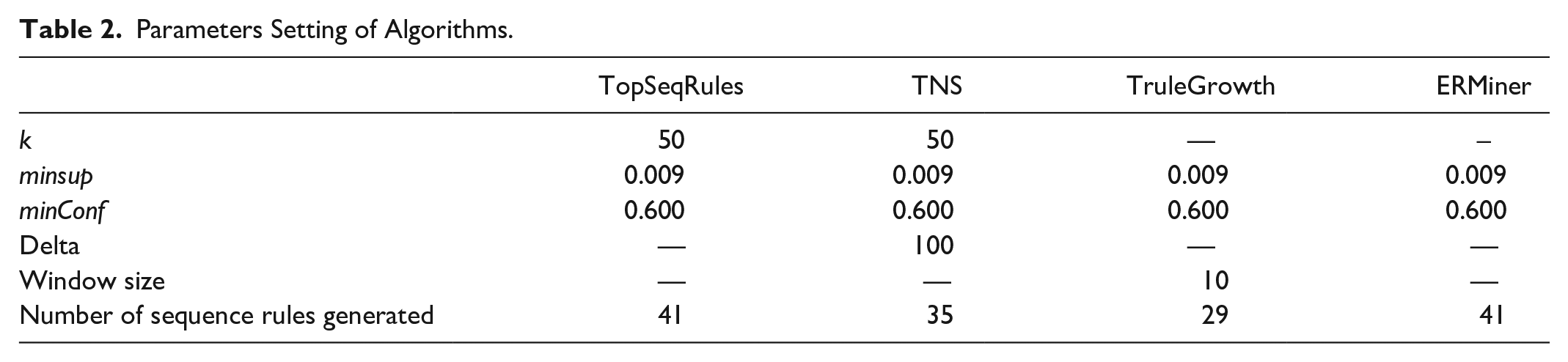
After running these algorithms, a set of sequential rules were generated with the rules with the higher Support and Confidence being almost the same. One critical issue in sequential pattern mining is to choose the threshold for the values of Support and Confidence, which depends on the data. For some datasets, there could be no rules with a Support of 0.9, while for other datasets, there could be millions of rules having a Support of 0.1. As a rule of thumb, we can start with some strict parameter settings like minSup = 0.9 and then decrease the parameter until we generate meaningful rules. If too many rules are generated, it is possible to set the parameters more strictly. Increasing the minSup will reduce the number of rules, and decreasing the minSup will increase the number of rules. In our datasets, the minSup was 0.009, which is higher than the value (0.006) in Vu et al. (2018). The minCof is set to be 0.6, a commonly used threshold in the literature (Jameel 2018; Naulaerts et al. 2015; Wu, Zhang, and Zhou 2019).

Findings

Stage one findings

Figure 2 is a heat map showing popular areas that international visitors visited during the Commonwealth Games and Figure 3 shows the number of international tourists at suburb level. In Figure 2, the bigger the bubble, the larger the number of tweets was recorded during the period of interest. There are six main concentrations, four of which correspond to the location of the games venues. The highest number of tweets was recorded in the Carrara Precinct, including two main games venues—Carrara Sports and Leisure Centre, and Carrara Stadium. The other three are Southport (the Athletes village), Nerang (Mountain Bike Trails), and Broadbeach (Bowls Club, Convention and Exhibition Centre, and transit center). The remaining hot spots are Bundall (major transport route) and Surfers Paradise (tourist center).

Figure 3.

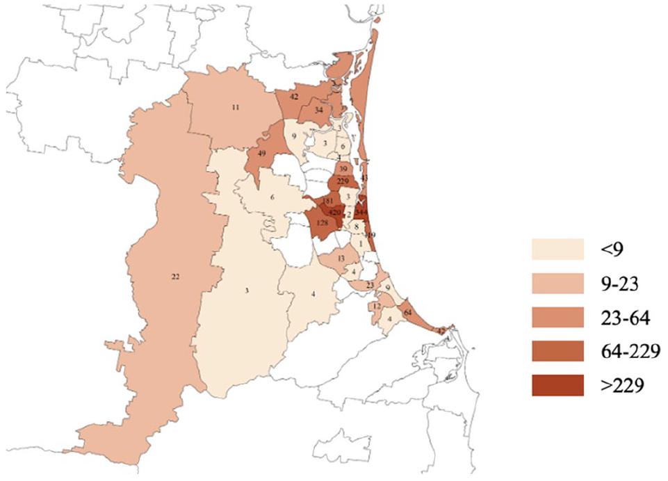
International users per suburb.

Figure 4 illustrates the international tourist dispersal during the event. The daily dispersal patterns demonstrate the shift of hotspots from one day to another, with day one showing a modest dispersal to the inland area and day two and three a more clustered concentration of the key games locations.

Figure 4.

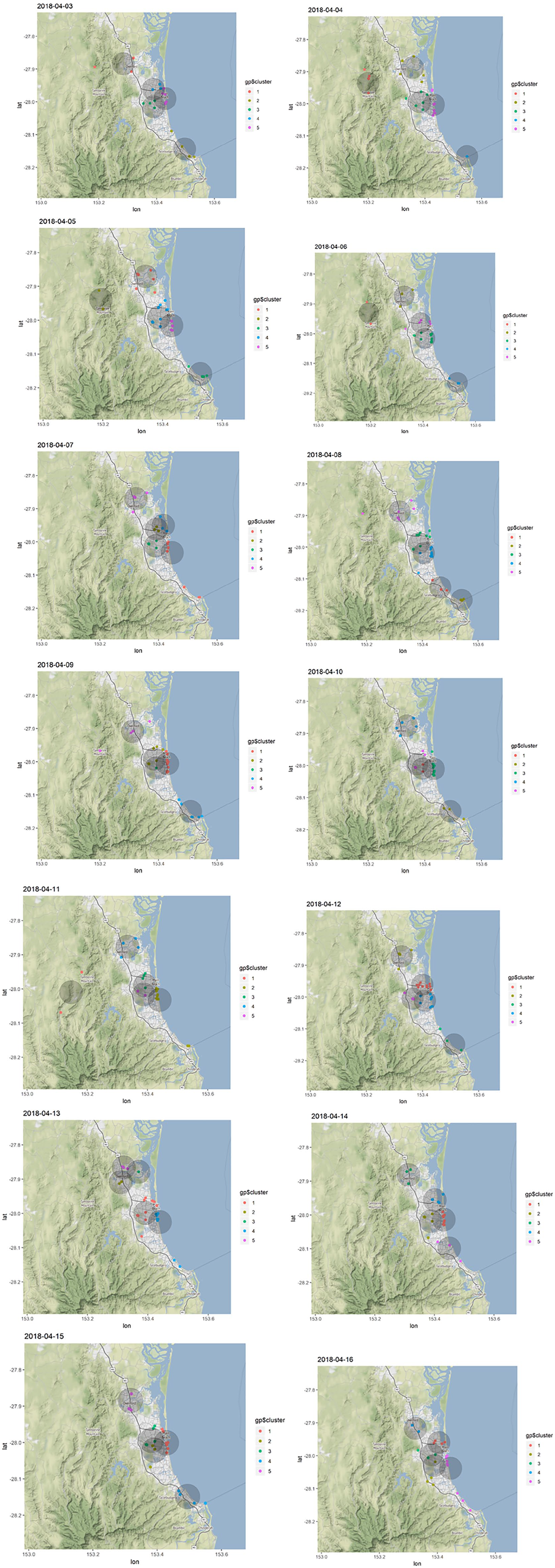
International users’ daily dispersal.

Based on the sequential patterns of their tweets, Figure 5 depicts the movement of the top 50 tourists by the number of tweets. It is evident that the international visitors’ movement is largely confined to the coastal areas, which are the city’s business and recreation centers. There is limited dispersal to the inland area where a variety of tourist attractions and activities exist.

Figure 5.

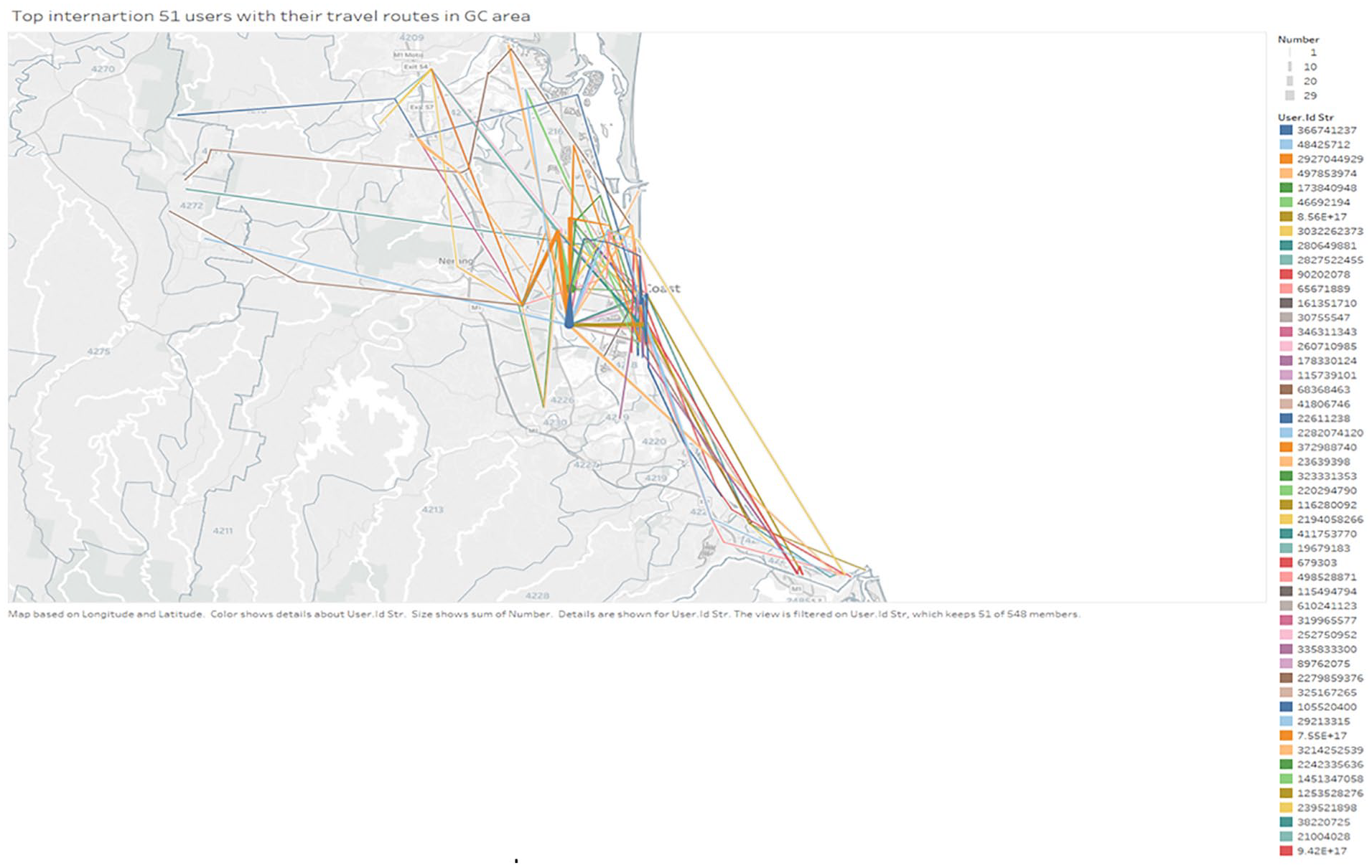
Travel routes of top 50 international users by the number of tweets.

Travel sequential analysis results

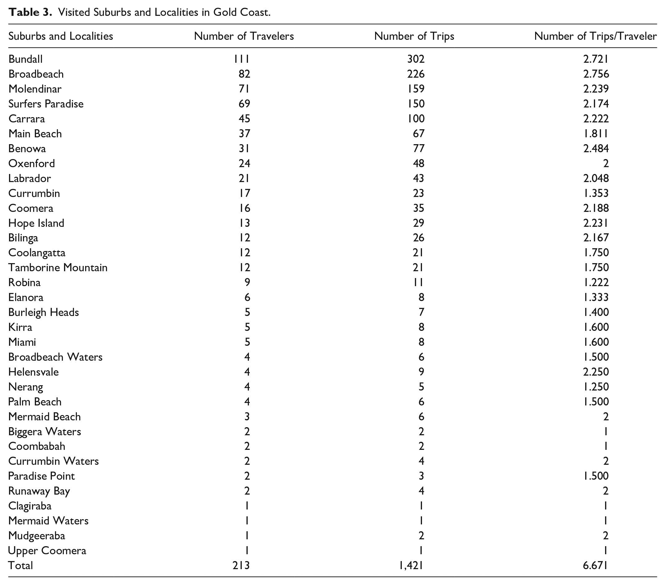
To identify sequential rules, only those 213 travel sequences that involve two or more suburbs were considered for further analysis. The final data set including 1,421 travel observations of 213 users is examined to capture travel behavior with respect to different suburbs and localities in and around the Gold Coast, which is shown in Table 3. Further, the 213 tourists’ demographics are shown in Table 4.

Table 3.

Visited Suburbs and Localities in Gold Coast.

Suburbs and Localities	Number of Travelers	Number of Trips	Number of Trips/Traveler
Bundall	111	302	2.721
Broadbeach	82	226	2.756
Molendinar	71	159	2.239
Surfers Paradise	69	150	2.174
Carrara	45	100	2.222
Main Beach	37	67	1.811
Benowa	31	77	2.484
Oxenford	24	48	2
Labrador	21	43	2.048
Currumbin	17	23	1.353
Coomera	16	35	2.188
Hope Island	13	29	2.231
Bilinga	12	26	2.167
Coolangatta	12	21	1.750
Tamborine Mountain	12	21	1.750
Robina	9	11	1.222
Elanora	6	8	1.333
Burleigh Heads	5	7	1.400
Kirra	5	8	1.600
Miami	5	8	1.600
Broadbeach Waters	4	6	1.500
Helensvale	4	9	2.250
Nerang	4	5	1.250
Palm Beach	4	6	1.500
Mermaid Beach	3	6	2
Biggera Waters	2	2	1
Coombabah	2	2	1
Currumbin Waters	2	4	2
Paradise Point	2	3	1.500
Runaway Bay	2	4	2
Clagiraba	1	1	1
Mermaid Waters	1	1	1
Mudgeeraba	1	2	2
Upper Coomera	1	1	1
Total	213	1,421	6.671

Table 4.

Tourist Demographics.

Continents	Number of Travelers	Percentages
Asia	33	15.5
Europe	107	50.2
The Americas	37	17.4
Africa	12	5.6
Australia/Oceania	24	11.3
Total	213	100

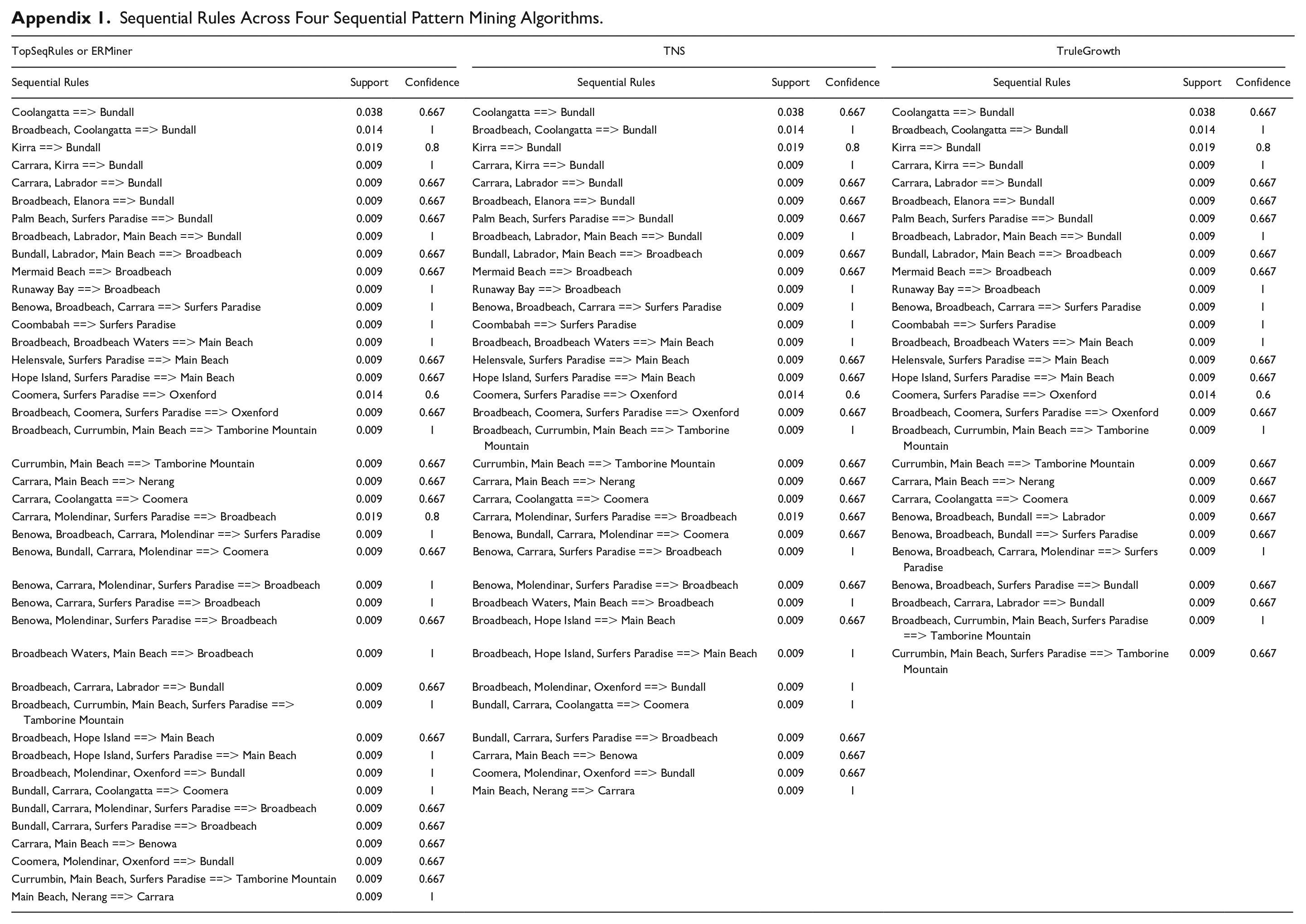
As illustrated in Table 2, the TopSeqRules, TNS, TruleGrowth, and ERMiner algorithms generate 41, 35, 29, and 41 sequence rules, respectively (see Appendix 1). Twenty-two sequential rules were identified, as reported in Table 5. Three of the authors independently read and analyzed the tweets associated with respective sequential pattern rules and then compared and discussed the results with each other until a final agreement was reached.

Table 5.

Sequential Rules by Subdivision.

Rule	Sequential Rules	Support	Confidence
r1	Coolangatta ==> Bundall	0.038	0.667
r2	Broadbeach, Coolangatta ==> Bundall	0.014	1
r3	Kirra ==> Bundall	0.019	0.800
r4	Carrara, Kirra ==> Bundall	0.009	1
r5	Carrara, Labrador ==> Bundall	0.009	0.667
r6	Broadbeach, Elanora ==> Bundall	0.009	0.667
r7	Palm Beach, Surfers Paradise ==> Bundall	0.009	0.667
r8	Broadbeach, Labrador, Main Beach ==> Bundall	0.009	1
r9	Bundall, Labrador, Main Beach ==> Broadbeach	0.009	0.667
r10	Mermaid Beach ==> Broadbeach	0.009	0.667
r11	Runaway Bay ==> Broadbeach	0.009	1
r12	Benowa, Broadbeach, Carrara ==> Surfers Paradise	0.009	1
r13	Coombabah ==> Surfers Paradise	0.009	1
r14	Broadbeach, Broadbeach Waters ==> Main Beach	0.009	1
r15	Helensvale, Surfers Paradise ==> Main Beach	0.009	0.667
r16	Hope Island, Surfers Paradise ==> Main Beach	0.009	0.667
r17	Coomera, Surfers Paradise ==> Oxenford	0.014	0.600
r18	Broadbeach, Coomera, Surfers Paradise ==> Oxenford	0.009	0.667
r19	Broadbeach, Currumbin, Main Beach ==> Tamborine Mountain	0.009	1
r20	Currumbin, Main Beach ==> Tamborine Mountain	0.009	0.667
r21	Carrara, Main Beach ==> Nerang	0.009	0.667
r22	Carrara, Coolangatta ==> Coomera	0.009	0.667

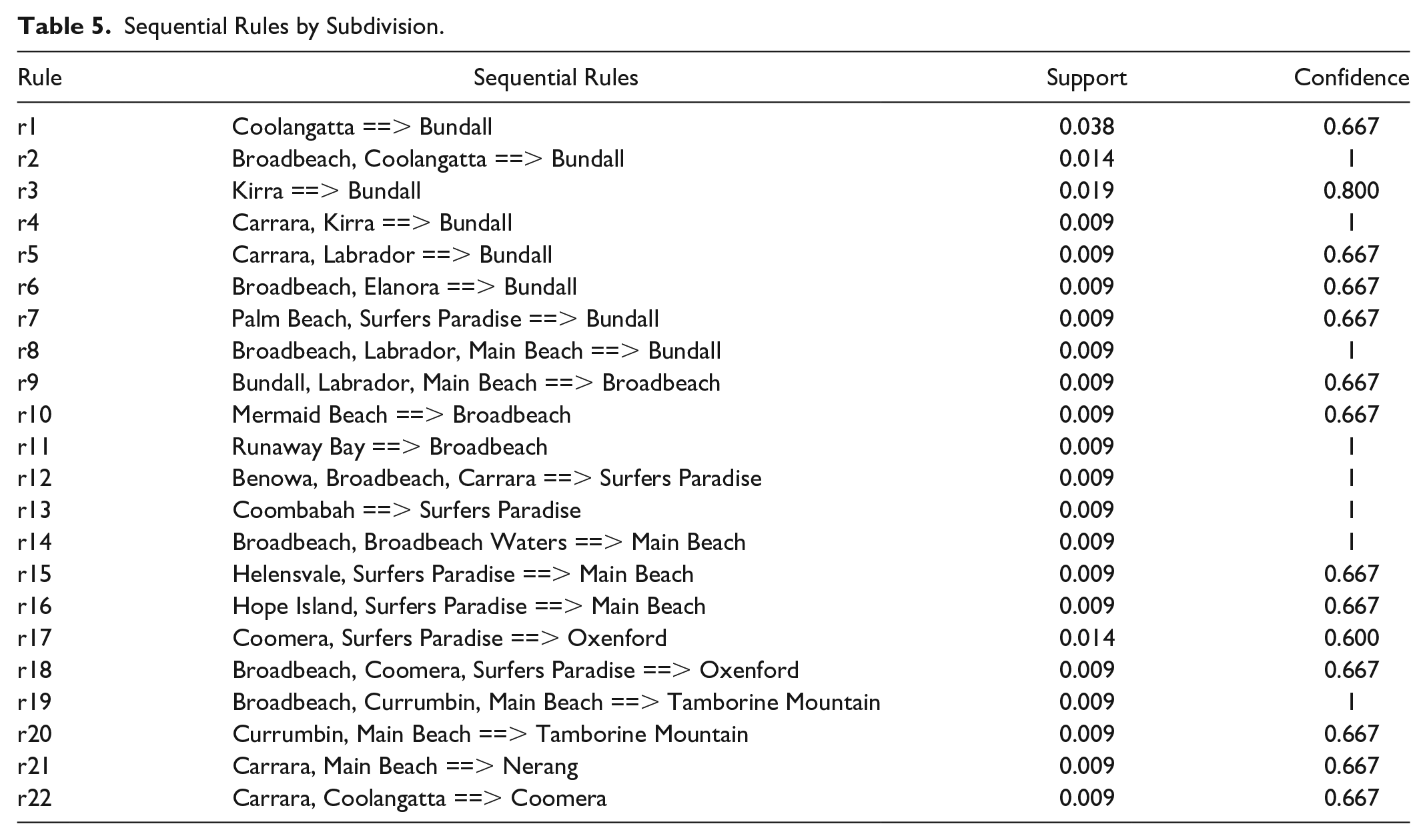
Table 5 shows that tourists in the sample have a high tendency to travel to Bundall, Broadbeach, Surfers Paradise, Main Beach, Oxenford, Tamborine Mountain, Nerang, and Coomera, with the minimum Confidence of 0.6. As reflected by rules r_1–8, a number of these were found for the destination in Bundall. That is, if tourists visit Coolangatta, and/or Broadbeach, they have a high chance of also visiting Bundall (rule r_1–2). Those who visit Kirra have a higher tendency also to visit Bundall, with a Confidence of 0.8 (rule r₃). Tourists are likely to visit Bundall after visiting Carrara, Kirra, or Labrador (rule r_4,5). Bundall would likely be visited after the destination combinations of Broadbeach and Elanora (rule r₆), Palm Beach and Surfers Paradise (rule r₇). Travelers who visit Broadbeach, Labrador, and Main Beach, have a high possibility to also visit Bundall next (rule r₈).

Also, Broadbeach, Surfers Paradise, Main Beach, Oxenford, and Tamborine Mountain are all popular tourism areas. Rule r₉ shows tourists who visit Bundall, Labrador, and Main Beach, will continue to visit Broadbeach. Tourists have a high chance of traveling to Broadbeach if they plan to visit Mermaid Beach or Runaway Bay (rules r₁₀ and r₁₁). Some strong sequential associations with the area of Surfers Paradise are identified. For instance, tourists have a high tendency to visit Benowa, Broadbeach, and Carrara first, and then Surfers Paradise next (rule r₁₂). Rule r₁₃ indicates that tourists who visit Coombabah have a high tendency to visit Surfers Paradise.

Rules r_14–16 indicate relatively strong sequential associations between the combinations of suburbs and Main Beach, such as Broadbeach and Broadbeach Waters, Helensvale and Surfers Paradise, Hope Island, and Surfers Paradise. Though the combinations are various, Main Beach is often the last destination. Rules r_17,18 show the possibility for tourists to visit Oxenford after Coomera and Surfers Paradise, or after Broadbeach, Coomera, and Surfers Paradise. Rules r_19,20 indicate Tamborine Mountain is likely to be visited after Broadbeach, Currumbin, and Main Beach, or after Currumbin and Main Beach. Lastly, rules r₁₀ and r₁₁ show the probability of 0.667 for tourists to visit Nerang after Carrara and Main Beach, and to visit Coomera after Carrara and Coolangatta.

Discussion and Conclusion

Theoretical and Practical Implications

Using the case study of GC2018, this paper addresses an important topic in the tourist movement literature in relation to mega events. The study extends upon the current literature in several ways. First, it approached tourist movement from the perspective of a suburb-level destination by extending the methodological literature through utilizing the geotagged social media data. While previous studies on sequential pattern mining (e.g., Vu et al. 2015, 2018) have considered the temporal and sequential dimensions of tourist movement, they have focused on country level and a general tourist context. Moreover, while Bermingham and Lee (2014) have highlighted the value of sequential pattern mining in uncovering the unobserved link between localities, their study only focuses on testing the effectiveness of sequential pattern mining using one algorithm. Our study contributes to extant tourism literature not only by empirically testing four different algorithms to ensure the reliable and meaningful identification of travel patterns but also by building knowledge on tourist dispersal at a suburb level within a specific destination.

More importantly, the study goes beyond Vu et al.’s (2018) early work by providing a detailed and empirically tested guideline for the four different algorithms, including TopSeqRules, TNS, TruleGrowth, and ERMiner, to discover the sequential association between the visited suburbs and localities to identify the shared patterns, which enables the extraction of more accurate sequential patterns. Table 6 shows the comparison between the four algorithms to showcase how to utilize them and how to achieve the best outcome when performing sequential pattern mining. TopSeqRules and TNS algorithms are the optimizations of classical sequential rule mining, while TruleGrowth and ERMiner algorithms are both extensions of the RuleGrowth algorithm. Further, these differences are mainly reflected in the input parameters, the generation of a desired amount of sequential rule, and the memory consumption and execution time in the running process. As Table 6 shows, each of the algorithms has their own pros and cons in identifying the sequential patterns in terms of their output and input. As such, to have the best outcomes of sequential pattern mining, a combination of these algorithms are recommended. As this study shows, the use of the four algorithms provides a more complete, reliable and accurate dispersal trajectory of tourist movement at international events. In contrast, Vu et al.’s (2018) study only uses TopSeqRules algorithm to investigate outbound tourism behavior at the national level with thirty days as the breakpoint.

Table 6.

Comparison Between Four Sequential Pattern Mining Algorithms.

	TopSeqRules	TNS	TruleGrowth	ERMiner
Output
Mining the top-k most frequent sequential rules	√	√	×	×
Mining the top-k most frequent non-redundant sequential rules	×	√	×	×
Mining sequential rules with a window size constraint	×	×	√	×
Mining sequential rules by applying the data structure named SCM and the equivalence classes	×	×	×	√
Input
A set of sequences	√	√	√	√
A K, the number of sequential rules	√	√	×	×
A Δ, increasing the chances of having an exact result	×	√	×	×
A min-sup threshold	×	×	√	√
A min-conf threshold	√	√	×	×
Window_size	×	×	√	×
Performance evaluation
Lower memory consumption	√, k dependent	√, k, Δ dependent	√	×
Faster execution time	√, k dependent	√, k, Δdependent	√	√

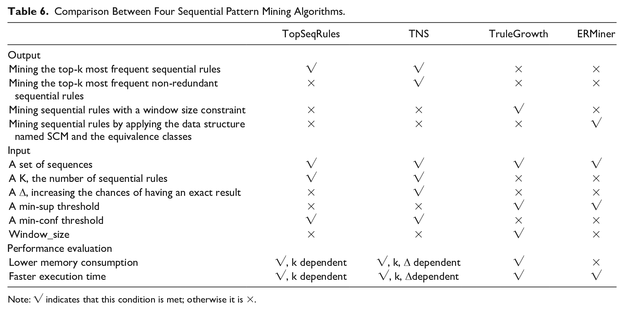
Note: √ indicates that this condition is met; otherwise it is ×.

Moreover, the current study conceptualizes what is referred to as the transit area in the tourist movement literature. Extant literature has discussed transit areas often in relation to passenger movement in transportation and occasionally in events as a way to improve the design and capacity in transit centers or the efficiency of the transport system (e.g., Khattak, Yangsheng, and Abid 2018; Ruan et al. 2016), but how such transit areas are conceptualized in tourist movement literature remain under-developed. In fact, transit area, as a concept, has been traditionally linked to transit tourism, where a stopover occurs between tourist generation region and destination region based on Leiper’s (1979) Tourism System (Poon and Ho 2021). This conceptualization usually focuses on the airport hub in the gateway cities (McKercher and Tang 2004; Poon and Ho 2021), failing to adequately explain the distinctiveness of transit area in the micro context within a destination beyond the transport network. Our conceptualization assumes that the event space and the way that tourists move in and out of it goes beyond transport networks—it is influenced by a range of factors including event scheduling and destination attractions. It addresses the call by McKercher, Filep, and Moyle (2021) to consider the seemingly continuous failure to acknowledge the concept of time expenditure, that is the trade-off between the time spent in transit and at an attraction or event and where the creation of transit areas can be a scarce resource.

In addition, this study captures the travel pattern of international visitors during the Commonwealth games between subdivisions in Gold Coast by constructing travel sequences at a more micro level—based on a set of coordinates, rather than macro levels such as country and city (e.g., Vu et al. 2018), which also broadens the application context of sequential rule mining in tourism literature. Thus, the study provides an advance on the current tourism and hospitality methodological and tourist dispersal literature by offering a more systematic, and objective approach for measuring tourist dispersal, serving as a reference for future research in understanding phenomenon. Table 7 identifies the contribution of the present study in comparison to the extant tourism literature.

Table 7.

Comparison Between This Research and Existing Studies on Tourist Movement.

Study	Research Setting	Research Method	Destination Level	Ordered Temporal Dimension	Data Source	Sample	Data Points	Analytics Methods
Current study	Mega event	Sequential pattern mining	Suburbs	√	Social media-Twitter	547 International visitors with 1,884 tweets	213 Travel sequences	TopSeqRules, TNS, TruleGrowth, and ERMiner algorithms
Gu et al. (2021)	Wine region in China	Time geography	Attractions (scenic spots and wineries)	√	GPS apps tracking and a questionnaire	790 Wine tourists	274 Useful questionnaires with GPS data	Spatial proximity and clustering + space-time prism model + ANOVA
Chen et al. (2021)	Global mobility of Chinese visitors from Sydney to other regions	Sankey diagrams	Countries/regions	×	Social media-Weibo	1,263 Weibo users	23,210 Posts	Frequency of geo-coordinates of posts
Hardy et al. (2020)	Tourist dispersal in the island state of Tasmania	Pearson correlation and OLS linear regression	State	×	GPS and survey	1,102 Tourists	396 Tourists	OLS linear regression
Zeng (2018)	Chinese tourist flow in Japan	Social network analysis	Cities and regions	×	Online travel group + Mafengwo and Ctrip	Chinese tourists	430 Travel itineraries and 458 trip diaries	Node structure and network structure
Vu et al. (2018)	Australian outbound tourism	Sequential rule mining	Countries	√	Social media-Flickr	809,313 Photos taken by 3,623 users	4,369 travel diaries	Top-K SRM algorithm
Chua et al. (2016)	Cilento	Trajectory mining and tourist detection	—	×	Social media-Twitter	3,135 Unique individuals	72,031 Geotagged tweets	Trajectory mining and tourist detection
Vu et al. (2015)	Hong Kong inbound tourism	Geographic information systems	Coordinators within the city	√	Social media-Flickr	2,100 International tourists	29,443 Geotagged photos	Density clustering + Markov Chain technique
Leung et al. (2012)	The 2008 Beijing Olympic Games	Content analysis and social network analysis	Attractions	×	Six different websites	International tourists	500 Online trip diaries	Content analysis and social network analysis

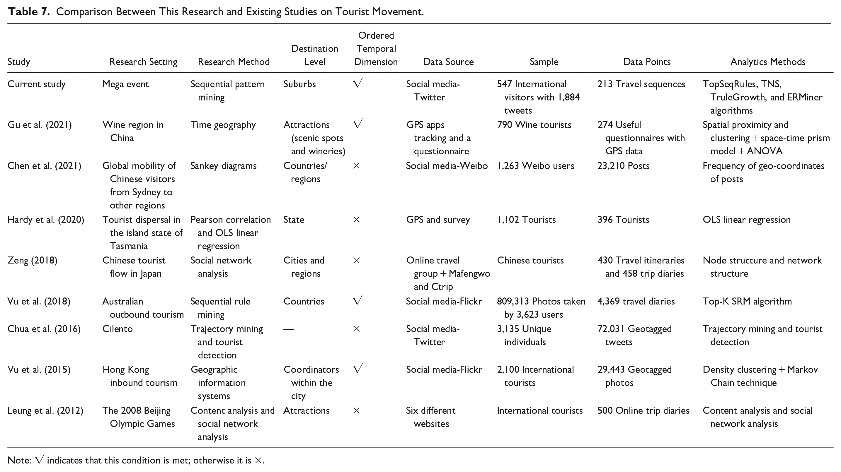
Note: √ indicates that this condition is met; otherwise it is ×.

Practically, the findings offer important implications for tourism destinations and event organizers. While comparing GC2018 K-means clustering results (Figure 4) and the tourists’ travel patterns (Tables 3 and 5) against the game transportation network (Figure 1), we found that tourists appeared to have followed the zoning and transport network and did not seem to venture much beyond areas around the main venues. For example, most of the visited localities listed on Tables 3 and 5 are within the core games route network (GRN), as specified in Figure 4. Localities with a lesser relation to the games were found to be less visited, despite that some are popular local tourist areas (e.g., Tamborine Mountain). Indeed, venues have a significant influence over event tourists’ dispersal. More importantly, the transit suburbs in the Gold Coast highlight the need to effectively capture the transit areas, where strategies can be built into by tapping into these transit areas by including relevant tourism resources and facilities. There can be a single modal road network or a multi-modal transit network in transportation planning for events. The sequential pattern analysis suggests the existence of transit areas, which are areas between points of interest in tourists’ movement in the event context. The data produced in this research are not sufficient to indicate the travel mode of tourists to understand the nature of their coverage of these areas. We are not certain whether tourists just pass through, or they may temporarily stay in these transit areas for leisure activities. It is possible that they visit the areas because they are convenient for sitting in a vehicle for social media posting while on their way to another location. However, based on the clear identification of these transit areas, event and city planners may consider how to best use these transit areas to disperse tourists’ expenditure and their visits in a host city. This is especially important when venues for a mega event scatter and multi-modal transports and transits are involved. In destinations lacking efficient and comprehensive public transport systems such as the Gold Coast, identifying the geographical coverage of tourists and predicting their next visit locations is beneficial for event planning.

In addition, the results of the sequential pattern mining offer empirical evidence for the purpose itinerary planning and for developing strategies around destination management organization. Tourism Research Australia (2019) notes that “we do not know what we do not know” (p. 4). Sequential pattern mining helps group pieces of past visitors’ journeys and helps to predict what tourists with similar profiles are likely to do next. This has significant implications by providing hard evidence on the development of recent automatic itinerary planning tools on “what you might also like.” For example, if tourists have visited Coomera and Surfers Paradise, Oxenford will likely be their next choice, which can be easily fed into automatic itinerary planning tools, as “when faced with many decision and uncertainties, people chose the path of least resistance” (Tourism Research Australia 2019, 4).

Methodological Reflections and Potential Remedies for Future Research

While the current study demonstrates methodological innovation, a number of pros and cons were identified. First, it provides an alternative to conventional methods for investigating tourist dispersal, typically involving the use of a survey and GPS techniques. These methods usually require face-to-face contact with tourists, resulting in limited response rates and geographical coverage (Vu et al. 2018). The advantages of our approach are the capacity to substantially enlarge the sample size without excessive cost, not bounded by the event sites, nor the provision of geo-location tracking devices that need to be supplied by researchers. However, researchers have less control over the scope and quality of the data, which vary across different social media platforms. As such, there is a need to be cautious of the potential response bias. We are cognizant of the fact that social media users (in this case Twitter) might not be representative of the population of all international tourists attending an event. An issue that has traditionally existed in social media research regarding the interpretation of findings (Olteanu et al. 2019). Common solutions to address this issue are to run longitudinal, multiple datasets, cross-domain analyses, or use of a range of approaches. Considering that this study is in an event context, future research using a combination of traditional methods, such as surveying conference attendees, would complement the findings of this research.

Second, unlike other methods, sequential mining offers critical insights into not only the locations but also the sequence in which these locations were visited by tourists. While we did not present the exact timing of the visit to locations, such information is attainable by cross-referencing the time information with geo-locations. A potential issue is to ascertain the exact geo-tag information of those tweets posted if the Twitter users are at the border between two neighboring suburbs. While geo-tag tweets, as Twitter suggests, provide the highest level of location precision to an exact location, previous research using geo-location images suggests an accuracy of up to 10–20 m (Hauff 2013; Xu et al. 2012). However, an increase in data size can enhance the method’s ability to comprehensively capture visited locations. There are also other opportunities for cross-referencing between geo-tag and other variables, such as user characteristics.

Third, the method has predictive power, which assists with the planning and management of events and tourism destinations. However, it does not reveal details on tourist expenditure and specific activities that visitors engage in to enable an impact analysis. Although tweet content provides some materials for interpretation, researchers need to be aware that content does not always align with location (i.e., a user may tweet about an activity undertaken in another location) and with limited information. Despite this, the method provides a cost-effective way to identify locations where tourism impacts are likely to occur. In addition, traditional approaches predominantly use surveys or GPS tracking devices to record tourist movement. Surveys largely rely on tourists’ memory to record where they have been. This can lead to potential bias as tourists might not remember or simply provide incorrect responses (Edwards et al. 2010). GPS devices can accurately record tourist movement; however, the analysis is largely descriptive and lacks predictive power. As such, sequential pattern mining’s power lies in its extraction of “previously unknown valuable patterns from a massive number of spatial-temporal trajectories” (Bermingham and Lee 2014, 379).

Another methodological contribution of our study on sequential pattern mining is to create the guidelines for determining the threshold for both min Support and Confidence for selecting rules. Essentially, the min Support and Confidence for sequential pattern mining depends on the data and how meaningful the rules are. Our study shows that there are three principles that need to be taken into consideration, these include: (1) use a combination of four algorithms until common rules are identified, (2) with reference to the existing literature—the minimum of support in the study of Vu et al. (2018) is 0.006, which is lower than our minsup (0.009). The minCof setting at 0.6 is a commonly used threshold in the literature (Jameel 2018; Naulaerts et al. 2015; Wu, Zhang, and Zhou 2019; (3) expert judgment to validate whether the rules are meaningful.

In summary, by using four sequential pattern mining algorithms, this research provides insights into tourist dispersal during major events. It differs from existing research by focusing mainly on actual behavior without predictive analysis, serving as a point of reference for future research in understanding tourist dispersal at mega events. Practically, it helps the event governing and planning bodies to understand tourist travel patterns and behaviors during events to assist future planning and resource allocation. It is useful for the industry to evaluate visitation to tourist attractions and the relative economic impact of the visitor flow on local communities and sub-regions (Chen 2021).

Limitations

While recognizing the important contributions of this study, it is not without limitations. First, we only used geo-tag to identify international visitors during the event. We assume that Twitter posters who registered in an international location and posted about GC2018 within the captured area were international tourists. It remains unknown whether the posters purchased tickets and attended the games as a spectator or in any other forms. Second, our data excluded visitors that posted on other social media sites or those who did not share their experiences or opinions on social media. Thus, caution is needed when extrapolating the findings to all GC2018 visitors. In this study, only movement of visitors within the Gold Coast were captured. Future studies may find ways to capture data on visitors’ trajectories at the pre and post event so that the economic, social, and environmental impact (spill-over) of a mega event on other regions of the host country could be estimated. Considering the sample size used in sequential pattern mining, to the best of the authors’ knowledge, there is no agreement over the minimum sample size (number of sequences) to perform the analysis. After a review of the existing literature and consulting the developer of the sequential pattern mining algorithm, there is compelling evidence that sequential pattern mining using small sample sizes can still achieve accurate and fast results (see Raïssi and Poncelet 2007). The sample size from our review ranges from 89 (e.g., Shyur, Jou, and Chang 2013) to a few thousand sequences (e.g., Bermingham and Lee 2014, 2,445 sequences). Further research to test the results of a range of sample sizes would offer important methodological insights into sequential pattern mining. In addition, considering the context of this study—one based on a mega event—future research using a combination of traditional methods alongside social media data, such as surveying event attendees and GPS could be used to triangulate and complement the findings of this research (McKercher, Filep, and Moyle 2021). Moreover, as COVID-19 is highly transmissible in crowds and indoor venues, it is very likely that tourists will move differently when visiting a destination to avoid crowding as protection against COVID-19. In that vein, future research that examines the movement of tourists before and during COVID-19 will offer insights into tourist movement during a time of global health crisis.

Footnotes

Appendix

Appendix 1.

Sequential Rules Across Four Sequential Pattern Mining Algorithms.

TopSeqRules or ERMiner			TNS			TruleGrowth
Sequential Rules	Support	Confidence	Sequential Rules	Support	Confidence	Sequential Rules	Support	Confidence
Coolangatta ==> Bundall	0.038	0.667	Coolangatta ==> Bundall	0.038	0.667	Coolangatta ==> Bundall	0.038	0.667
Broadbeach, Coolangatta ==> Bundall	0.014	1	Broadbeach, Coolangatta ==> Bundall	0.014	1	Broadbeach, Coolangatta ==> Bundall	0.014	1
Kirra ==> Bundall	0.019	0.8	Kirra ==> Bundall	0.019	0.8	Kirra ==> Bundall	0.019	0.8
Carrara, Kirra ==> Bundall	0.009	1	Carrara, Kirra ==> Bundall	0.009	1	Carrara, Kirra ==> Bundall	0.009	1
Carrara, Labrador ==> Bundall	0.009	0.667	Carrara, Labrador ==> Bundall	0.009	0.667	Carrara, Labrador ==> Bundall	0.009	0.667
Broadbeach, Elanora ==> Bundall	0.009	0.667	Broadbeach, Elanora ==> Bundall	0.009	0.667	Broadbeach, Elanora ==> Bundall	0.009	0.667
Palm Beach, Surfers Paradise ==> Bundall	0.009	0.667	Palm Beach, Surfers Paradise ==> Bundall	0.009	0.667	Palm Beach, Surfers Paradise ==> Bundall	0.009	0.667
Broadbeach, Labrador, Main Beach ==> Bundall	0.009	1	Broadbeach, Labrador, Main Beach ==> Bundall	0.009	1	Broadbeach, Labrador, Main Beach ==> Bundall	0.009	1
Bundall, Labrador, Main Beach ==> Broadbeach	0.009	0.667	Bundall, Labrador, Main Beach ==> Broadbeach	0.009	0.667	Bundall, Labrador, Main Beach ==> Broadbeach	0.009	0.667
Mermaid Beach ==> Broadbeach	0.009	0.667	Mermaid Beach ==> Broadbeach	0.009	0.667	Mermaid Beach ==> Broadbeach	0.009	0.667
Runaway Bay ==> Broadbeach	0.009	1	Runaway Bay ==> Broadbeach	0.009	1	Runaway Bay ==> Broadbeach	0.009	1
Benowa, Broadbeach, Carrara ==> Surfers Paradise	0.009	1	Benowa, Broadbeach, Carrara ==> Surfers Paradise	0.009	1	Benowa, Broadbeach, Carrara ==> Surfers Paradise	0.009	1
Coombabah ==> Surfers Paradise	0.009	1	Coombabah ==> Surfers Paradise	0.009	1	Coombabah ==> Surfers Paradise	0.009	1
Broadbeach, Broadbeach Waters ==> Main Beach	0.009	1	Broadbeach, Broadbeach Waters ==> Main Beach	0.009	1	Broadbeach, Broadbeach Waters ==> Main Beach	0.009	1
Helensvale, Surfers Paradise ==> Main Beach	0.009	0.667	Helensvale, Surfers Paradise ==> Main Beach	0.009	0.667	Helensvale, Surfers Paradise ==> Main Beach	0.009	0.667
Hope Island, Surfers Paradise ==> Main Beach	0.009	0.667	Hope Island, Surfers Paradise ==> Main Beach	0.009	0.667	Hope Island, Surfers Paradise ==> Main Beach	0.009	0.667
Coomera, Surfers Paradise ==> Oxenford	0.014	0.6	Coomera, Surfers Paradise ==> Oxenford	0.014	0.6	Coomera, Surfers Paradise ==> Oxenford	0.014	0.6
Broadbeach, Coomera, Surfers Paradise ==> Oxenford	0.009	0.667	Broadbeach, Coomera, Surfers Paradise ==> Oxenford	0.009	0.667	Broadbeach, Coomera, Surfers Paradise ==> Oxenford	0.009	0.667
Broadbeach, Currumbin, Main Beach ==> Tamborine Mountain	0.009	1	Broadbeach, Currumbin, Main Beach ==> Tamborine Mountain	0.009	1	Broadbeach, Currumbin, Main Beach ==> Tamborine Mountain	0.009	1
Currumbin, Main Beach ==> Tamborine Mountain	0.009	0.667	Currumbin, Main Beach ==> Tamborine Mountain	0.009	0.667	Currumbin, Main Beach ==> Tamborine Mountain	0.009	0.667
Carrara, Main Beach ==> Nerang	0.009	0.667	Carrara, Main Beach ==> Nerang	0.009	0.667	Carrara, Main Beach ==> Nerang	0.009	0.667
Carrara, Coolangatta ==> Coomera	0.009	0.667	Carrara, Coolangatta ==> Coomera	0.009	0.667	Carrara, Coolangatta ==> Coomera	0.009	0.667
Carrara, Molendinar, Surfers Paradise ==> Broadbeach	0.019	0.8	Carrara, Molendinar, Surfers Paradise ==> Broadbeach	0.019	0.667	Benowa, Broadbeach, Bundall ==> Labrador	0.009	0.667
Benowa, Broadbeach, Carrara, Molendinar ==> Surfers Paradise	0.009	1	Benowa, Bundall, Carrara, Molendinar ==> Coomera	0.009	0.667	Benowa, Broadbeach, Bundall ==> Surfers Paradise	0.009	0.667
Benowa, Bundall, Carrara, Molendinar ==> Coomera	0.009	0.667	Benowa, Carrara, Surfers Paradise ==> Broadbeach	0.009	1	Benowa, Broadbeach, Carrara, Molendinar ==> Surfers Paradise	0.009	1
Benowa, Carrara, Molendinar, Surfers Paradise ==> Broadbeach	0.009	1	Benowa, Molendinar, Surfers Paradise ==> Broadbeach	0.009	0.667	Benowa, Broadbeach, Surfers Paradise ==> Bundall	0.009	0.667
Benowa, Carrara, Surfers Paradise ==> Broadbeach	0.009	1	Broadbeach Waters, Main Beach ==> Broadbeach	0.009	1	Broadbeach, Carrara, Labrador ==> Bundall	0.009	0.667
Benowa, Molendinar, Surfers Paradise ==> Broadbeach	0.009	0.667	Broadbeach, Hope Island ==> Main Beach	0.009	0.667	Broadbeach, Currumbin, Main Beach, Surfers Paradise ==> Tamborine Mountain	0.009	1
Broadbeach Waters, Main Beach ==> Broadbeach	0.009	1	Broadbeach, Hope Island, Surfers Paradise ==> Main Beach	0.009	1	Currumbin, Main Beach, Surfers Paradise ==> Tamborine Mountain	0.009	0.667
Broadbeach, Carrara, Labrador ==> Bundall	0.009	0.667	Broadbeach, Molendinar, Oxenford ==> Bundall	0.009	1
Broadbeach, Currumbin, Main Beach, Surfers Paradise ==> Tamborine Mountain	0.009	1	Bundall, Carrara, Coolangatta ==> Coomera	0.009	1
Broadbeach, Hope Island ==> Main Beach	0.009	0.667	Bundall, Carrara, Surfers Paradise ==> Broadbeach	0.009	0.667
Broadbeach, Hope Island, Surfers Paradise ==> Main Beach	0.009	1	Carrara, Main Beach ==> Benowa	0.009	0.667
Broadbeach, Molendinar, Oxenford ==> Bundall	0.009	1	Coomera, Molendinar, Oxenford ==> Bundall	0.009	0.667
Bundall, Carrara, Coolangatta ==> Coomera	0.009	1	Main Beach, Nerang ==> Carrara	0.009	1
Bundall, Carrara, Molendinar, Surfers Paradise ==> Broadbeach	0.009	0.667
Bundall, Carrara, Surfers Paradise ==> Broadbeach	0.009	0.667
Carrara, Main Beach ==> Benowa	0.009	0.667
Coomera, Molendinar, Oxenford ==> Bundall	0.009	0.667
Currumbin, Main Beach, Surfers Paradise ==> Tamborine Mountain	0.009	0.667
Main Beach, Nerang ==> Carrara	0.009	1

Acknowledgements

The first three authors have contributed equally and should be regarded as co-first authors.

Declaration of Conflicting Interests

The author(s) declared no potential conflicts of interest with respect to the research, authorship, and/or publication of this article.

Funding

The author(s) disclosed receipt of the following financial support for the research, authorship, and/or publication of this article: The author/s would like to acknowledge the financial support from Griffith University Commonwealth Games Research Projects Scheme.

ORCID iDs

Mingming Cheng

Xin Jin

Xiaowei Wang

Jinyan Chen

Author Biographies

Dr Mingming Cheng is an Associate Professor in Digital Marketing and Research Lead of the Social Media Research Lab in the School of Management and Marketing at Curtin University, Australia. His research examines the digital transformation of the tourism industry - new experiences (e.g., Airbnb), new marketing channels (e.g., social media), new technology-savvy markets (e.g., Chinese post-80s tourist market) and more recently, environmental impacts of tourism including carbon footprint.

Dr Xin Jin is Senior Lecturer of Department of Tourism, Sport and Hotel Management, Griffith Business School, Griffith University. Her two main areas of research interest are event tourism and destination marketing.

Dr Ying Wang is an Associate Professor with the School of Hotel and Tourism Management, Hong Kong Polytechnic University. Her research interests include destination management and marketing, travel technologies, Chinese tourism, and HRM in hotels.

Dr Xiaowei Wang is a lecturer at the School of Tourism and Urban-rural Planning at Zhejiang Gongshang University, China. Her research interests include peer-to-peer accommodation, tourism marketing and big data analytics.

Dr Jinyan Chen is a Research Assistant Professor in the School of Hotel and Tourism Management, Hong Kong Polytechnic University. Her research interests include tourist mobility, sentiment analysis, social media and big data in tourism management.

References

Bauder

Freytag

2015. “Visitor Mobility in the City and the Effects of Travel Preparation.” Tourism Geographies 17 (5): 682–700.

Becken

Wilson

2013. “The Impacts of Weather on Tourist Travel.” Tourism Geographies 15 (4): 620–39.

Bermingham

Lee

2014. “Spatio-Temporal Sequential Pattern Mining for Tourism Sciences.” Procedia Computer Science 29: 379–89.

Caldeira

A. M.

Kastenholz

2020. “Spatiotemporal Tourist Behaviour in Urban Destinations: A Framework of Analysis.” Tourism Geographies 22 (1): 22–50.

Chen

2021. Construction of Green Supply Chain in Rural Tourism and Its Coordination Mechanism: Perspective of Front-Back Stage Structure. Wuhan: Huazhong University of Science & Technology Press.

Chen

Becken

Stantic

2021. “Using Weibo to Track Global Mobility of Chinese Visitors.” Annals of Tourism Research 89: 103078.

Chua

Servillo

Marcheggiani

Moere

A. V.

2016. “Mapping Cilento: Using Geotagged Social Media Data to Characterize Tourist Flows in Southern Italy.” Tourism Management 57: 295–310.

Couper

2000. “Web Surveys: A Review of Issues and Approaches.” Public Opinion Quarterly 64 (4): 464–94.

East

Osborne

Kemp

Woodfine

2017. “Combining GPS & Survey Data Improves Understanding of Visitor Behaviour.” Tourism Management 61: 307–20.

10.

Edwards

Dickson

Griffin

Hayllar

2010. “Tracking the Urban Visitor: Methods for Examining Tourists’ Spatial Behaviour and Visual Representations.” In Cultural Tourism Research Methods, edited by Richards

Munsters

, 104–14. Oxford: CABI Publishing.

11.

Edwards

Griffin

2013. “Understanding Tourists’ Spatial Behaviour: GPS Tracking as an Aid to Sustainable Destination Management.” Journal of Sustainable Tourism 21 (4): 580–95.

12.

Epstein

Quinn

2020. “Markers of Online Privacy Marginalization: Empirical Examination of Socioeconomic Disparities in Social Media Privacy Attitudes, Literacy, and Behavior.” Social Media + Society 6 (2): 2056305120916853.

13.

Fourie

Santana-Gallego

2011. “The Impact of Mega-Sport Events on Tourist Arrivals.” Tourism Management 32 (6): 1364–70.

14.

Fournier-Viger

Gomariz

Gueniche

Soltani

C. W.

Tseng

V. S.

2014b. “SPMF: A Java Open-Source Pattern Mining Library.” The Journal of Machine Learning Research 15 (1): 3389–93.

15.

Fournier-Viger

C. W.

Tseng

V. S.

Cao

Nkambou

2015. “Mining Partially-Ordered Sequential Rules Common to Multiple Sequences.” IEEE Transactions on Knowledge and Data Engineering 27 (8): 2203–16.

16.

Fournier-Viger

C. W.

Tseng

V. S.

Nkambou

2012b. “Mining Sequential Rules Common to Several Sequences With the Window Size Constraint.” Paper presented at the Canadian Conference on Artificial Intelligence, May, 299–304. Berlin, Heidelberg: Springer.

17.

Fournier-Viger

Gueniche

Zida

Tseng

V. S.

2014a. “ERMiner: Sequential Rule Mining Using Equivalence Classes.” Paper presented at the International Symposium on Intelligent Data Analysis, October, 108–19. Cham: Springer.

18.

Fournier-Viger

Faghihi

Nkambou

Nguifo

E. M.

2012a. “CMRules: Mining Sequential Rules Common to Several Sequences.” Knowledge-Based Systems 25 (1): 63–76.

19.

Fournier-Viger

Tseng

V. S.

2011. “Mining Top-k Sequential Rules.” Paper presented at the Advanced Data Mining and Applications: 7th International Conference, December, 180–94. Berlin, Heidelberg: Springer.

20.

Fournier-Viger

Tseng

V. S.

2013. “TNS: Mining Top-k Non-Redundant Sequential Rules.” Paper presented at the Proceedings of the 28th Annual ACM Symposium on Applied Computing, March, 164–6.

21.

Zhang

Huang

Zheng

Chen

2021. “Tourists’ Spatiotemporal Behaviors in an Emerging Wine Region: A Time-Geography Perspective.” Journal of Destination Marketing & Management 19: 100513.

22.

Hallo

J. C.

Manning

R. E.

Valliere

Budruk

2004. “A Case Study Comparison of Visitor Self-Reported and GPS Recorded Travel Routes.” Paper presented at the Proceedings of the 2004 Northeastern Recreation Research Symposium, March–April, 172–7.

23.

Hardy

Birenboim

Wells

2020. “Using Geoinformatics to Assess Tourist Dispersal at the State Level.” Annals of Tourism Research 82: 102903.

24.

Hauff

2013. “A Study on the Accuracy of Flickr’s Geotag Data.” Paper presented at the Proceedings of the 36th International ACM SIGIR Conference on Research and Development in Information Retrieval, July, 1037–40.

25.

Jameel

N. G. M.

2018. “SMS Spam Detection Using Association Rule Mining Based on SMS Structural Features.” Journal of Theoretical and Applied Information Technology 96 (12): 3962–72.

26.

Jin

Cheng

2020. “Communicating Mega Events on Twitter: Implications for Destination Marketing.” Journal of Travel & Tourism Marketing 37 (6): 739–55.

27.

Khattak

Yangsheng

Abid

M. M.

2018. “Optimal Configuration of the Metro Rail Transit Station Service Facilities by Integrated Simulation-Optimization Method Using Passengers’ Flow Fluctuation.” Arabian Journal for Science and Engineering 43 (10): 5499–516.

28.

Koo

T. T. R.

C. L.

Dwyer

2010. “Ground Travel Mode Choices of Air Arrivals at Regional Destinations: The Significance of Tourism Attributes and Destination Contexts.” Research in Transportation Economics 26 (1): 44–53.

29.

Koo

T. T. R.

C. L.

Dwyer

2012. “Dispersal of Visitors Within Destinations: Descriptive Measures and Underlying Drivers.” Tourism Management 33 (5): 1209–19.

30.

Koo

T. T. R.

Lau

P. L.

Dwyer

2017. “The Geographic Dispersal of Visitors: Insights From the Power Law.” Journal of Travel Research 56 (1): 108–21.

31.

Leiper

1979. “The Framework of Tourism: Towards a Definition of Tourism, Tourist, and the Tourist Industry.” Annals of Tourism Research 6 (4): 390–407.

32.

Leung

X. Y.

Wang

Bai

Stahura

K. A.

Xie

2012. “A Social Network Analysis of Overseas Tourist Movement Patterns in Beijing: The Impact of the Olympic Games.” International Journal of Tourism Research 14 (5): 469–84.

33.

Likas

Vlassis

Verbeek

J. J.

2003. “The Global k-Means Clustering Algorithm.” Pattern Recognition 36 (2): 451–61.

34.

Mabroukeh

N. R.

Ezeife

C. I.

2010. “A Taxonomy of Sequential Pattern Mining Algorithms.” ACM Computing Surveys 43 (1): 1–41.

35.

Mair

Chien

P. M.

Kelly

S. J.

Derrington

2021. “Social Impacts of Mega-Events: A Systematic Narrative Review and Research Agenda.” Journal of Sustainable Tourism. Published online January 12. doi:10.1080/09669582.2020.1870989.

36.

McKercher

Tang

2004. “The Challenges of Developing Transit Tourism.” Asia Pacific Journal of Tourism Research 9 (2): 151–60.

37.

Mckercher

Lau

2008. “Movement Patterns of Tourists Within a Destination.” Tourism Geographies 10 (3): 355–74.

38.

McKercher

Shoval

Birenboim

2012. “First and Repeat Visitor Behaviour: GPS Tracking and GIS Analysis in Hong Kong.” Tourism Geographies 14 (1): 147–61.

39.

McKercher

Shoval

Park

Kahani

2015. “The [Limited] Impact of Weather on Tourist Behavior in an Urban Destination.” Journal of Travel Research 54 (4): 442–55.

40.

McKercher

Filep

Moyle

2021. “Movement in Tourism: Time to Re-Integrate the Tourist?” Annals of Tourism Research 91: 103199.

41.

Naulaerts

Meysman

Bittremieux

T. N.

Vanden Berghe

Goethals

Laukens

2015. “A Primer to Frequent Itemset Mining for Bioinformatics.” Briefings in Bioinformatics 16 (2): 216–31.

42.

Nguyen

L. T. T.

Nguyen

L. T. T.

Fournier-Viger

Selamat

2017. “ETARM: An Efficient Top-k Association Rule Mining Algorithm.” Applied Intelligence 48 (5): 1148–60.

43.

Olteanu

Castillo

Diaz

Kıcıman

2019. “Social Data: Biases, Methodological Pitfalls, and Ethical Boundaries.” Frontiers in Big Data 2: 13.

44.

Pettersson

Getz

2009. “Event Experiences in Time and Space: A Study of Visitors to the 2007 World Alpine Ski Championships in Åre, Sweden.” Scandinavian Journal of Hospitality and Tourism 9 (2–3): 308–26.

45.

Pettersson

Zillinger

2011. “Time and Space in Event Behaviour: Tracking Visitors by GPS.” Tourism Geographies 13 (1): 1–20.

46.

Poon

P. C. M.

G. K. S.

2021. “Opportunities in Transit Tourism: A Case Study of Hong Kong as a Transit Destination.” Journal of Travel & Tourism Marketing 38 (1): 31–43.

47.

Prideaux

2000. “The Role of the Transport System in Destination Development.” Tourism Management 21 (1): 53–63.

48.

Queensland Government. 2018. “Gold Coast 2018 Commonwealth Games by Numbers.” May 1. http://statements.qld.gov.au/Statement/2018/5/1/gold-coast-2018-commonwealth-games-by-numbers.

49.

Raïssi

Poncelet

2007. “Sampling for Sequential Pattern Mining: From Static Databases to Data Streams.” Paper presented at the Seventh IEEE International Conference on Data Mining, October, 631–6.

50.

Raun

Ahas

Tiru

2016. “Measuring Tourism Destinations Using Mobile Tracking Data.” Tourism Management 57: 202–12.

51.

Ruan

J. M.

Liu

Wei

Zhu

Zhou

2016. “How Many and Where to Locate Parking Lots? A Space–Time Accessibility-Maximization Modeling Framework for Special Event Traffic Management.” Urban Rail Transit 2 (2): 59–70.

52.

Shoval

Kahani

De Cantis

Ferrante

2020. “Impact of Incentives on Tourist Activity in Space-Time.” Annals of Tourism Research 80: 102846.

53.

Shyur

H. J.

Jou

Chang

2013. “A Data Mining Approach to Discovering Reliable Sequential Patterns.” Journal of Systems and Software 86 (8): 2196–203.

54.

Sørensen

Sundbo

2014. “Potentials for User-Based Innovation in Tourism: The Example of GPS Tracking of Attraction Visitors.” In Handbook of Research on Innovation in Tourism Industries. Cheltenham: Edward Elgar Publishing.

55.

Tourism Research Australia. 2019. “The Beach, Bush and Beyond: Understanding Regional Dispersal of Australian Tourists.” https://www.destinationnsw.com.au/wp-content/uploads/2019/10/Understanding-Regional-Dispersal-of-Australian-tourists-October-2019.pdf.

56.

Townsend

Wallace

2016. Social Media Research: A Guide to Ethics. Aberdeen: University of Aberdeen.

57.

Twitter Inc. 2016. “Twitter Terms of Service.” https://twitter.com/en/tos/previous/version_10.

58.

Twitter Inc. 2021. “Twitter Terms of Service.” https://twitter.com/en/tos#intlTerms.

59.

Versichele

de Groote

Claeys Bouuaert

Neutens

Moerman

Van de Weghe

2014. “Pattern Mining in Tourist Attraction Visits Through Association Rule Learning on Bluetooth Tracking Data: A Case Study of Ghent, Belgium.” Tourism Management 44: 67–81.

60.

H. Q.

Law

B. H.

2015. “Exploring the Travel Behaviors of Inbound Tourists to Hong Kong Using Geotagged Photos.” Tourism Management 46: 222–32.

61.

H. Q.

Law

Zhang

2018. “Travel Diaries Analysis by Sequential Rule Mining.” Journal of Travel Research 57 (3): 399–413.

62.

Wang

Jin

2019. “Event-Based Destination Marketing: The Role of Mega-Events.” Event Management 23 (1): 109–18.

63.

C. L.

Carson

2008. “Spatial and Temporal Tourist Dispersal Analysis in Multiple Destination Travel.” Journal of Travel Research 46 (3): 311–7.

64.

D. Y.

Zhang

X. Y.

Zhou

X. L.

2019. “Properties and Therapeutic Efficacy of Chinese Materia Medica Based on Strategy Pattern.” Journal of Physics Conference Series 1207 (1): 012004.

65.

Xia

Zeephongsekul

Packer

2011. “Spatial and Temporal Modelling of Tourist Movements Using Semi-Markov Processes.” Tourism Management 32 (4): 844–51.

66.

Nash

Whitmarsh

2020. “Big Data or Small Data? A Methodological Review of Sustainable Tourism.” Journal of Sustainable Tourism 28 (2): 144–63.

67.

Mei

Zeng

Luo

2012. “Amigo: Accurate Mobile Image Geotagging.” Paper presented at the Proceedings of the 4th International Conference on Internet Multimedia Computing and Service, September, 11–4.

68.

Zeng

2018. “Pattern of Chinese Tourist Flows in Japan: A Social Network Analysis Perspective.” Tourism Geographies 20 (5): 810–32.